Applicability of Nonlinear Wavemaker Theory

Abstract

Generation of high-quality waves is essential when making numerical or physically model tests. When using a wavemaker theory outside the validity area, spurious waves are generated. In order to investigate the validity of different wave generation methods, new model test results are presented where linear and nonlinear wave generation theories are tested on regular and irregular waves. A simple modification to the second-order wavemaker theory is presented, which significantly reduces the generation of spurious waves when used outside its range of applicability. For highly nonlinear regular waves, only the ad-hoc unified wave generation based on stream function wave theory was found acceptable. For irregular waves, similar conclusions are drawn, but the modified second-order wavemaker method is more relevant. This is because the ad-hoc unified generation method for irregular waves requires the wave kinematics to be calculated by a numerical model, which might be quite time-consuming. Finally, a table is presented with the range of applicability for each wavemaker method for regular and irregular waves.

1. Introduction

When performing tests in laboratories or numerical models, high-quality waves representing conditions in prototype as close as possible is of highest priority. In the early 20th century, linear wavemaker theory was developed by Havelock [1], which was later extended to a fully second-order irregular wavemaker theory by Schäffer [2,3]. This extension made it possible to generate mildly nonlinear waves without spurious free waves. The spurious free waves contaminate the wave field and can easily be seen for regular waves for cases with low wave reflection, as the wave shape is not constant in space. For example, Orszaghova et al. [4] showed that using first-order wavemaker theory could lead to erroneously wave run-up and wave overtopping results compared to generating the waves with second-order wavemaker theory. Furthermore, Sriram et al. [5] showed that the breaking point of focused waves is different when using first-order and second-order wavemaker theory. This was expected to be caused by the influence from the free spurious long-wave components generated with first-order theory.

Recently, ad-hoc unified wavemaker theories were proposed by Zhang and Schäffer [6] for regular waves and by Zhang et al. [7] for irregular waves. These ad-hoc unified wave generation methods make it possible to generate highly nonlinear waves of high quality in intermediate and shallow water. These methods require a depth-averaged velocity as input to control the motion of the piston wavemaker. For regular waves, a fully nonlinear wave theory is available in the form of the stream function wave theory by Fenton and Rienecker [8], and from this, the depth-averaged velocity can be calculated. At the moment, there exists no analytical model to calculate the kinematics for highly nonlinear irregular waves, but the kinematics can be obtained by numerical models, for example, Boussinesq type wave models. The propagation of waves from deep to shallow water with numerical models can be time-consuming. Therefore, it is more efficient to use the first or second-order wavemaker theory for irregular waves when they are valid.

Unwanted free waves are generated when using a wavemaker theory outside its validity area. Schäffer [3] specified that the second-order wavemaker theory is not valid for regular waves when a secondary crest is produced in the wave trough. This happens when the second-order amplitude is larger than ¼ of the first-order amplitude. To describe this, he introduced the nonlinearity parameter, S which must not exceed unity for the second-order wavemaker theory to be valid. For regular waves, Schäffer [3] defined S as four times the ratio between the amplitudes of the second-order and the first-order components in regular waves and is given by:

$$\mathrm{S} = 2\left|{HG}_{\mathrm{nm}}^{\pm }\right|$$

(1)

where $G_{\mathrm{nm}}^{\pm }$ is the second-order surface elevation transfer function given for example in Schäffer [3], H is the wave height. For the application of Equation (1) on irregular waves Schäffer [3] proposed to use a characteristic wave height (H = H_1/3) and f_n = f_m = f_p to calculate $G_{\mathrm{nm}}^{\pm }$.

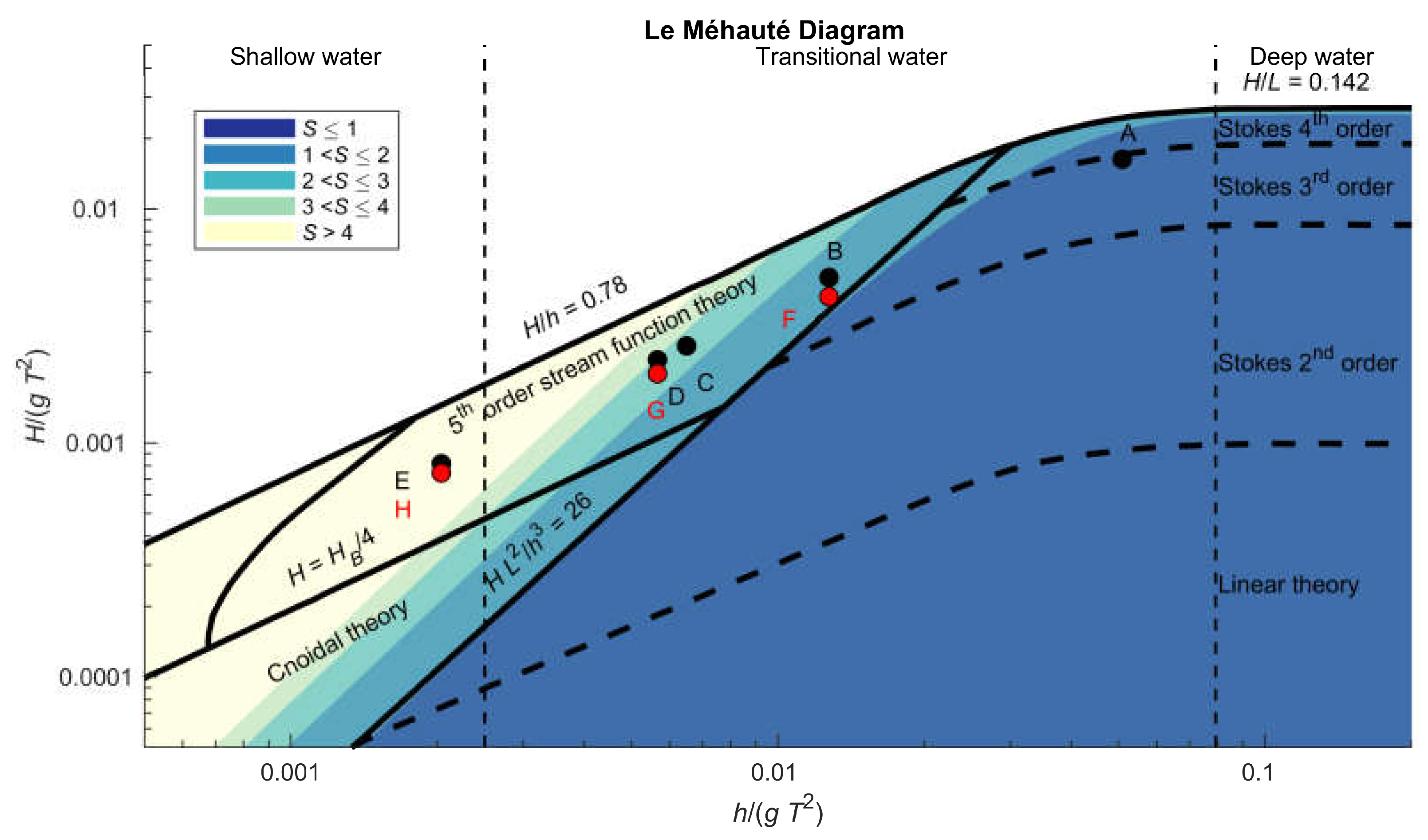
A more well-known approach to check the applicability of wave maker theories is the diagram by Le Méhauté [9], which described what wave theory was valid depending on the relative water depth and the wave steepness. Figure 1 shows an example of the Le Méhauté diagram and colored areas that illustrates different S ranges calculated with Equation (1). From the figure, it is seen that using the applicability criteria for second-order waves given by Schäffer [3] corresponds to fourth order Stokes waves according to the diagram by Le Méhauté [9]. This clearly shows the need of testing the applicability range of the existing methods and to provide some recommendations that can easily be followed.

The present paper presents new physical model test results to study the applicability of the different wavemaker methods for regular and irregular waves. A simple modification to the second-order wavemaker theory by Schäffer [3] is proposed to extend its range of applicability and to significantly reduce errors for highly nonlinear cases. Furthermore, recommendations are given for the validity of each of the tested wavemaker theories.

2. Present Study

New model tests covering linear to highly nonlinear waves have been performed in the new wave flume at Aalborg University for regular (5 tests) and irregular (3 tests) waves, see Figure 1.

The purpose of the tests is to study the applicability of each wavemaker theory and to provide a clear definition for the applicability range of each wavemaker theory. Furthermore, is it investigated if the applicability range of the second-order wavemaker theory can be extended with a simple modification. The second-order wavemaker theory is modified in the present paper by introducing a maximum allowed relation between the second-order amplitude and the first-order amplitude. This limitation is controlled by a S_max value, so for example, S_max = 1 means that the second-order amplitude will be reduced to ¼ of the first-order amplitude if it was predicted higher. Without this upper limit, the second-order amplitude might be even larger than the first-order amplitude which is physically incorrect. Instead the second-order component should saturate at a level smaller than the primary component and third and higher order components should increase instead.

The second-order components generated by two interacting components were scaled by introducing a more generalized form of S. This is done by rewriting Equation (1) to consider the two interacting components:

$${S(f}_{\mathrm{n}}{,f}_{\mathrm{m}}{) = HG}_{\mathrm{nm}}^{\pm }{/\mathsf{\delta }}_{\mathrm{nm}}$$

(2)

where f_n and f_m are the frequencies of the two interacting components. δ_nm is 0.5 for f_n = f_m and 1 for f_n ≠ f_m. In the present paper the characteristic wave height is on the safe side taken as the maximum wave height (H = 2H_m0 ≈ H_max).

The modification to the second-order wavemaker theory is performed by the scaling factor, λ, given by Equation (3).

$${\mathsf{\lambda }}_{\mathrm{nm}} =\min \left(1,\frac{S_{\max }}{S\left(f_{\mathrm{n}}{,f}_{\mathrm{m}}\right)}\right)$$

(3)

The scaling factor should be calculated for all interacting frequencies in the first-order wave spectra and be multiplied to both second-order transfer functions $G_{\mathrm{nm}}^{\pm }$ and $F_{\mathrm{nm}}^{\pm }$. $G_{\mathrm{nm}}^{\pm }$ is the transfer function for the second-order surface elevation and $F_{\mathrm{nm}}^{\pm }$ is the transfer function of the second-order paddle movement. This reduces the amount of second-order energy so no secondary crest is calculated for the interaction of the individual frequencies. The optimal value of S_max is expected in this interval (1 ≤ S_max ≤ 4) which corresponds to a second-order amplitude of 25–100% of the first-order amplitude. Although the criteria of S ≤ 1 given by Schäffer [3] is for superharmonics in regular waves the scaling is applied also to irregular waves. The present paper focus only on superharmonics ($G_{\mathrm{nm}}^{+}$ and $F_{\mathrm{nm}}^{+}$), but the scaling is expected necessary also to subharmonics ($G_{\mathrm{nm}}^{-}$ and $F_{\mathrm{nm}}^{-}$). Correct generation of the subharmonics is very important for response of many structures, but the present paper focus only on the superharmonics for which free energy is much easier to observe in the measured time series.

3. Theoretical Optimal S_max

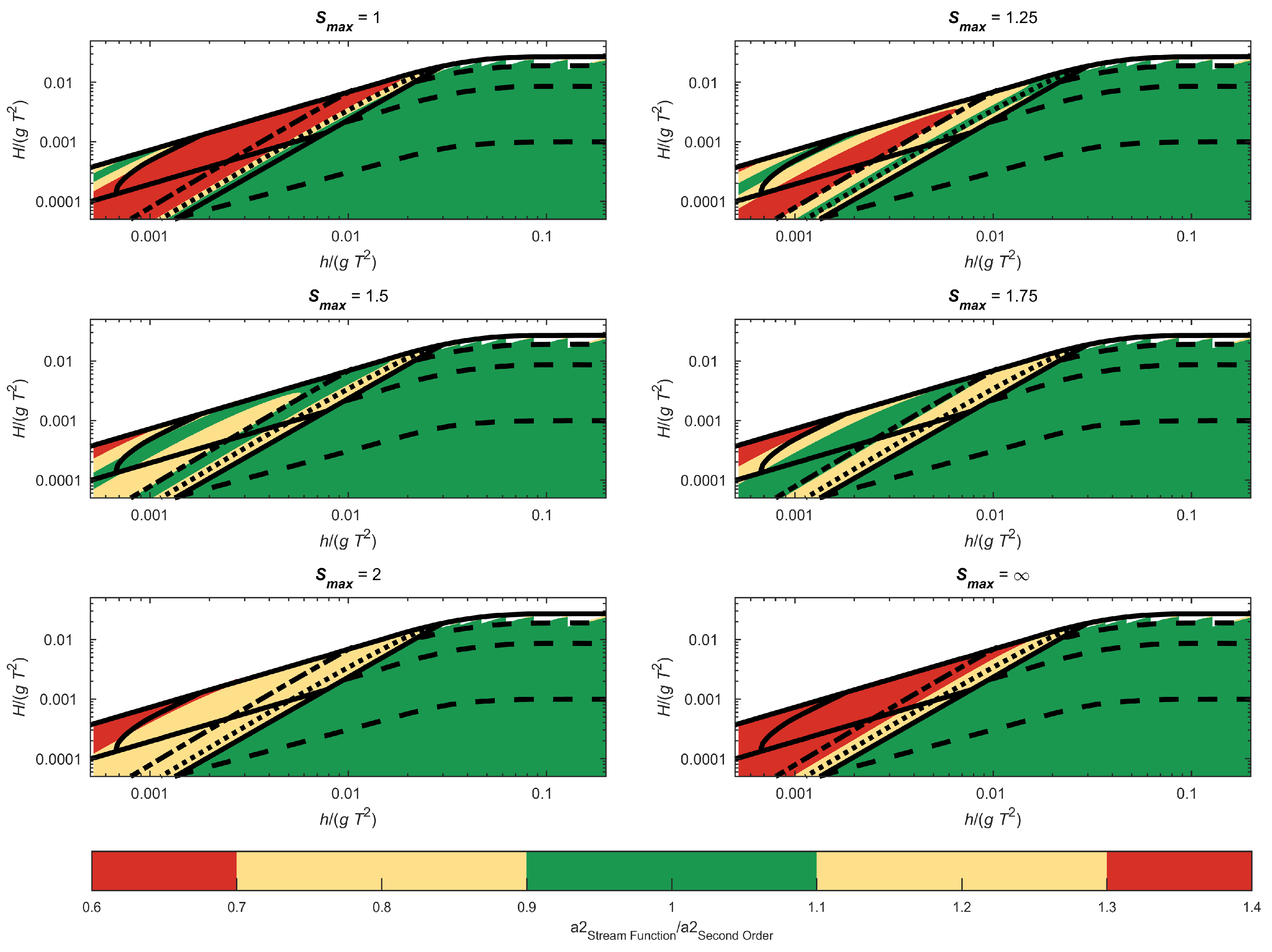
The nonlinear wave theory by Fenton and Rienecker [8] can estimate the correct amount of second-order energy that exists for a given regular wave over a horizontal sea bed. With the use of nonlinear wave theory, it is thus possible to estimate what artificial limit (S_max in Equation (3)) should be used in the second-order wave theory to obtain the best results. In Figure 2, the calculated amplitude of the second-order component by second-order wavemaker theory is compared with the calculated by stream function wave theory by Fenton and Rienecker [8]. This is done for different values of S_max, where S_max = ∞ corresponds to no limit on the second-order energy (unmodified Schäffer [3] method).

The given applicability range by Schäffer [3] (S ≤ 1) shows errors smaller than 10% when using the second-order wavemaker theory by Schäffer [3], see Figure 2. The figure shows that the recommendations given by Le Méhauté [9] based on this analysis might be on the safe side. However, this comparison though only considers the amplitude of the second-order component, but higher order components might be relevant.

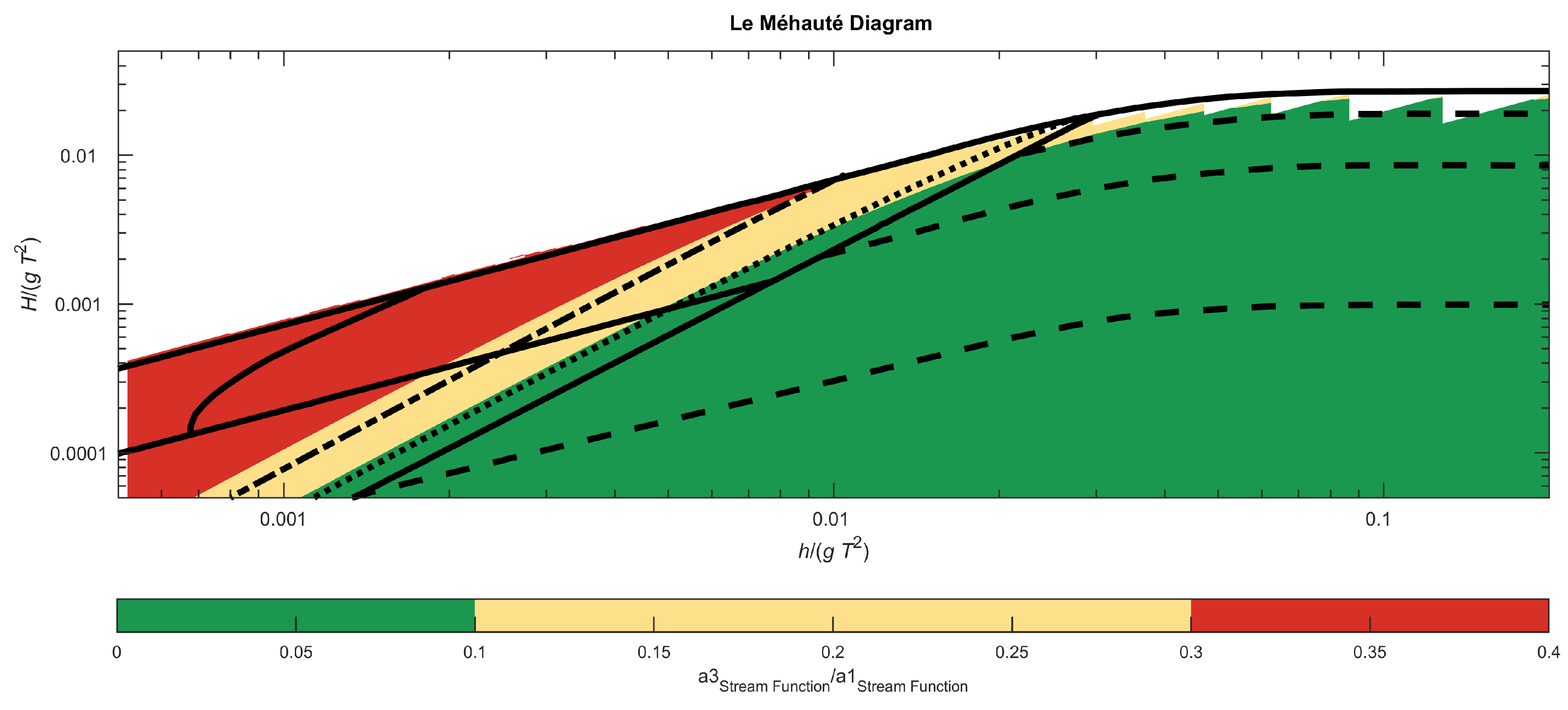
By limiting the second-order energy to S_max = 1 the modified second-order wave generation gives errors smaller than 10% for wave conditions up to S ≈ 1.5 as illustrated by the dotted line in the figure. Using values of S_max = 1.5–1.75 gives a larger area where the error is below 10%. Even though S_max = 1.5–1.75 gives a larger area where the second-order amplitude is calculated with a small error, the second-order wavemaker theory is not necessarily valid as the third, and higher order energy might have a significant contribution. Therefore, the relation between the second-order and third order components must additionally be small. In Figure 3, the third order amplitude is compared to the first-order amplitude calculated by stream function wave theory. The figure shows that for sea states with S ≤ 1.5 the amplitude of the third order component is below 10% of the first-order component. From these results, an optimum of S_max = 1 is found, and the expected range of applicability is extended from S = 1 to S = 1.5 with the modified second-order wavemaker theory.

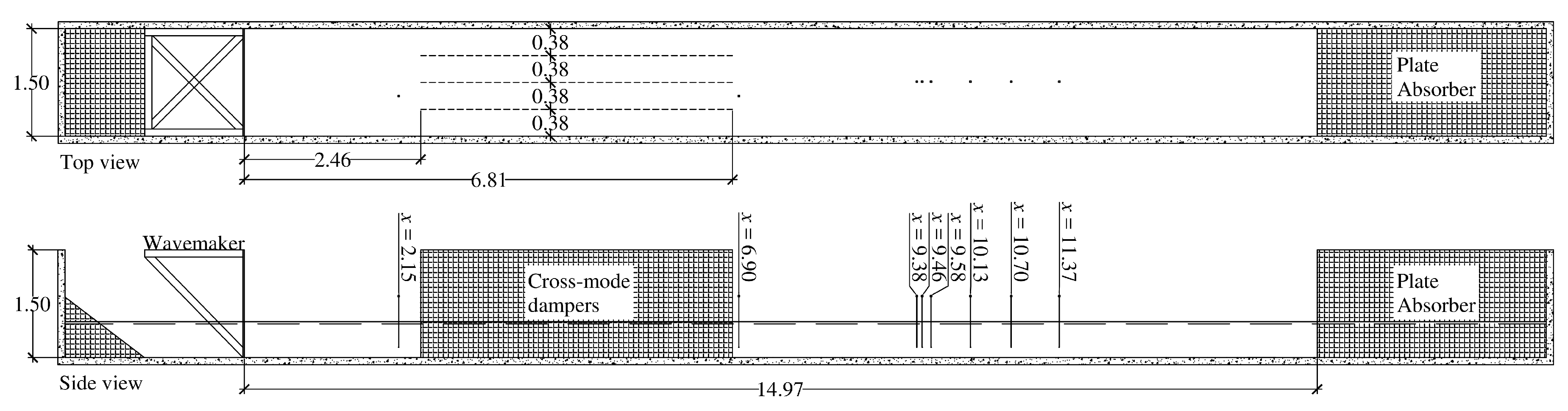
4. Model Test Setup and Methodology

To verify the results from Section 3, physically experiments have been performed where the surface elevation was measured in different locations in the wave flume, see Figure 4.

The flume is equipped with a piston-type wavemaker, cross-mode dampers and a passive absorption system with perforated sheets in the end of the flume. The cross-mode dampers are a permanent installation in the flume and not installed due to specific cross-mode problems with the generated waves in the present study. The wavemaker has two sets of flush mounted resistance wave gauge on the wave board, which is used to avoid re-reflected waves from the wave board with use of the active wave absorption method by Lykke Andersen et al. [10]. The active absorption system has proven also to be effective for nonlinear irregular waves, cf. Lykke Andersen et al. [11]. The control signals are thus the wavemaker position and the surface elevation in the nearfield.

To evaluate the validity of each wavemaker theory, the measured surface elevation is compared to the theoretical surface elevation. The regular waves are compared to the predicted surface elevation by Fenton and Rienecker [8] and the irregular waves are compared to the COULWAVE Boussinesq wave model by Lynett and Liu [12]. The COULWAVE model is an accurate model when it comes to shoal waves from deep to shallow water including nonlinear interactions, see [13,14]. The results from the COULWAVE model was also used to generate the input for the ad-hoc unified irregular wave generation method by Zhang et al. [7].

The COULWAVE model was used to propagate irregular waves from deep water to the water depth used in the laboratory (0.5 m). The water depth at the wavemaker in COULWAVE is a compromise between the wave regime where the model is valid, kh < 6, and that regime where first-order wavemaker theory can be used. The waves were generated in the COULWAVE model on a horizontal part using a narrow banded JONSWAP spectrum (γ = 10) and truncated at 0.5 to 1.5 times the peak frequency. Thus, the primary spectrum does not significantly overlap with the bound harmonics. Then followed a 1:100 slope to the depth of 0.5 m and finally a horizontal part with a water depth of 0.5 m. The point where the 1:100 slope end, the surface elevation time series was extracted and used as a target for the different wave generation methods. The last horizontal part is where the target values are extracted to be compared with the measured surface elevation in the laboratory.

Table 1. Wave conditions of the irregular waves at the generation point in COULWAVE.

	Model Parameters		Generation Point			h = 0.5 m
Case	Cells per Wavelength	Courant Number	h [m]	Hm0 [m]	TP [s]	Hm0 [m]
F	200	0.5	2.5	0.102	2	0.083
G	200	0.5	4.0	0.087	3	0.087
H	300	0.5	8.0	0.068	5	0.091

shows the numerical model parameters and the sea state conditions at the generation point and at h = 0.5 m.

The number of cells pr. wavelength is based on the wavelength of the peak wave period at the generation point. Thus, the discretisation of the model is, Δx = (cells per wavelength)/wavelength. The courant number is calculated by C = c₀Δt/Δx, where c₀ is the shallow water celerity at the generation point and Δt is the timestep.

The method by Zhang et al. [7] uses the averaged velocity in the wave direction, but since only the surface elevation is provided from the COULWAVE model, a conversion to depth-averaged velocity is performed by assuming shallow water wave theory being valid. That is not entirely correct in intermediate water, but a fair approximation.

Because the generated primary spectrum in COULWAVE is narrow banded and truncated (0.5 to 1.5 times the peak frequency), the primary components can be separated from the bound harmonics by bandpass filtering at 0.5 f_P < f < 1.5 f_P. This truncated spectrum was used as primary spectrum for the second-order wave generation method. The signal without bandpass was used as input for the method by Zhang et al. [7]. The measured waves in the laboratory were then compared with the unfiltered signals from the numerical model in the wave gauge locations.

The theoretical surface elevations calculated with COULWAVE and Fenton and Rienecker [8] might differ from the measured surface elevation due to the cross-mode dampers. The cross-mode dampers might slightly dissipate some of the energy in the physical flume. This is likely to be seen as a reduction in wave height when comparing the measured surface elevation at x = 2.15 m and x = 6.90 m. Furthermore, the theoretical surface elevation is without reflected waves which is difficult to entirely avoid in the physical model. Therefore, reflection in the experimental tests should be reduced to a minimum. The amplitude reflection coefficient in the physical tests was in the range of 11% to 16%, which was calculated with the nonlinear irregular wave separation method by Eldrup and Lykke Andersen [15]. The amount of reflection in the physical experiments is found acceptable for comparing the total measured surface elevation with the theoretical surface elevation.

5. Regular Wave Results

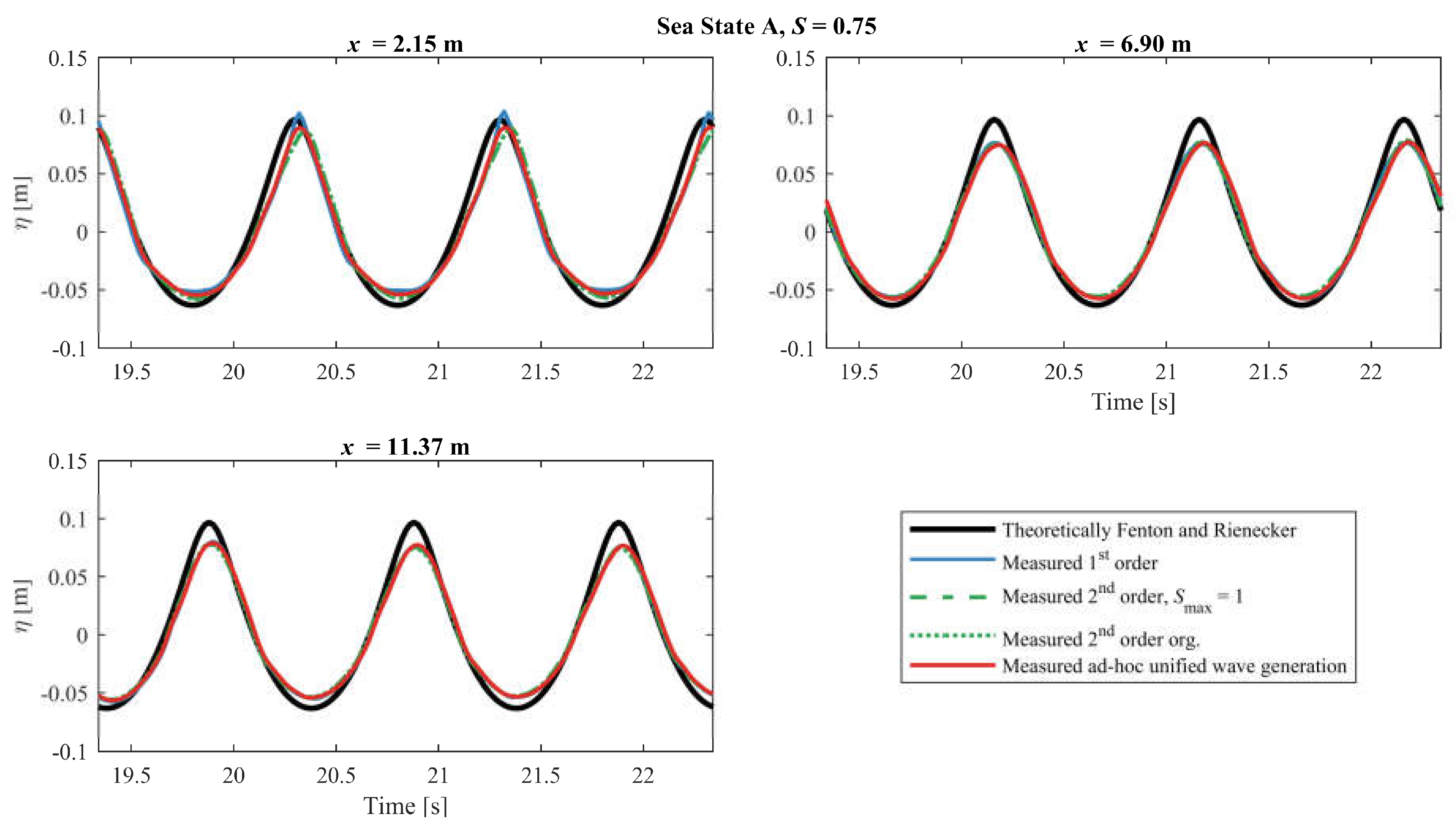
For regular waves, the different wavemaker theories are evaluated against the theoretical stream function wave theory. This evaluation is performed at different distances from the wavemaker. Linear to highly nonlinear waves were generated and compared to the theoretical wave profiles. The measured surface elevations are shown after the ramp-up of the wavemaker is completed and if possible before reflection is present in the signals.

Figure 5 shows the results for Sea State A. The measured profiles are almost identical for the different wave generation methods. However, a reduction in the amplitude is observed for x ≥ 6.90 m. The reduction in amplitude might be due to the cross-mode dampers. The shape of the measured surface elevations for all the wavemaker theories are similar to the theoretical. Therefore, it can be concluded that all the tested wavemaker methods are valid for Sea State A, and thus the first and second-order wave generation methods lead to acceptable waves, in a more extensive area than given by the Le Méhauté diagram. However, Sea State A is within the validity range given by Schäffer [3] (S < 1).

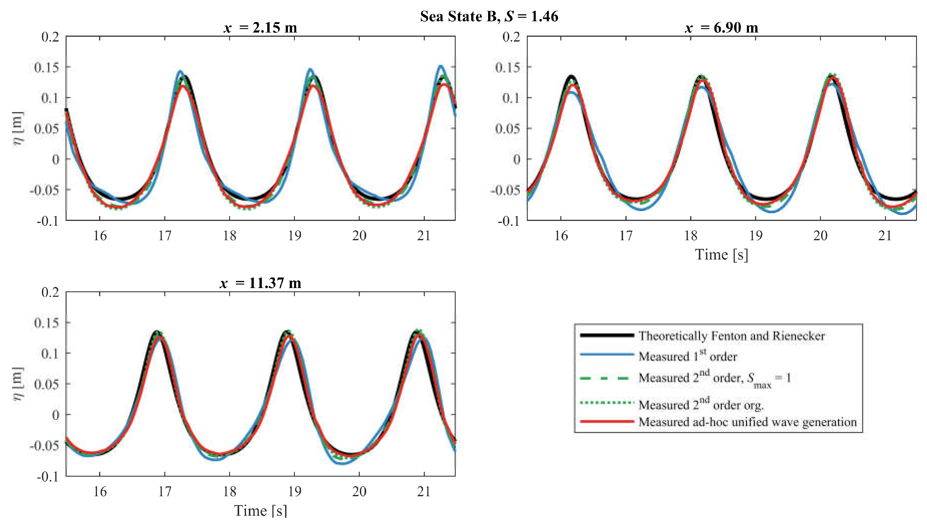
The results for Sea State B are shown in Figure 6 from which it appears that the first-order wavemaker method lead to some minor deviations in the wave shape, indicating some free higher harmonics energy exist. The surface profile for the second-order methods and the ad-hoc unified generation method are similar, and these are close to the theoretical profile. The wave height of the generated waves is slightly lower than the theoretical, but the wave shape is a close match to the target. From the section with the theoretical analysis of an optimum of S_max, a difference was expected to be seen between the original second-order and the modified second-order method when S > 1.0, but this is not observed from Figure 6 for a case with S = 1.46.

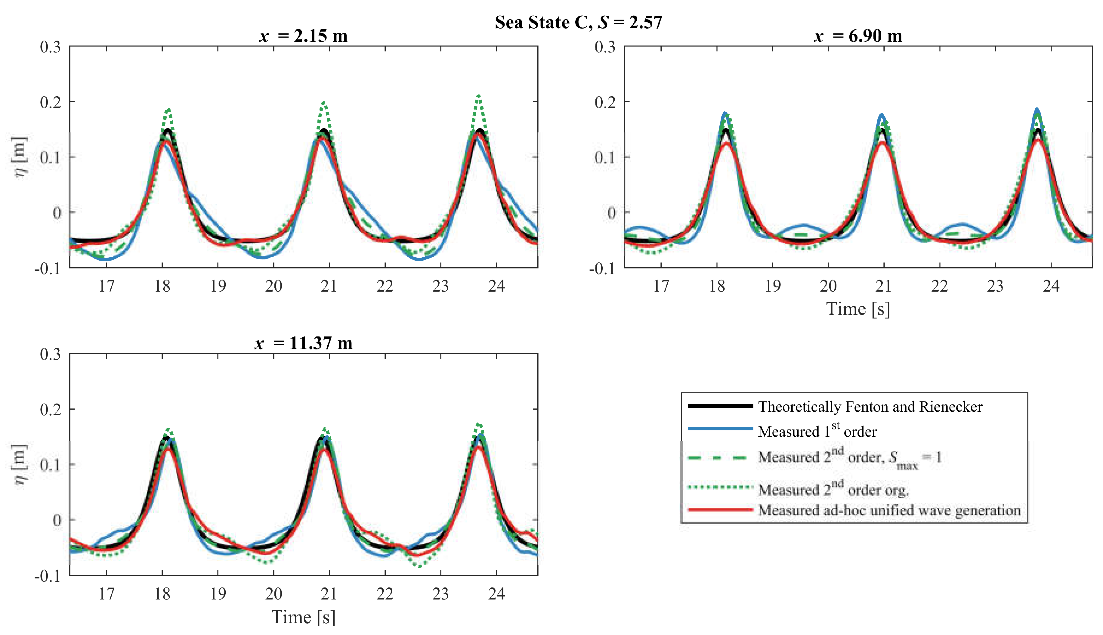
Results for Sea State C shows that the wave profile generated with first and second-order wavemaker theory is not constant in the various gauge positions, cf. Figure 7. This is due to free unwanted waves being generated by these theories when the nonlinearity is too high. The second-order wavemaker theory is slightly better than first-order theory, but the ad-hoc unified wave generation is a close match to the theoretical profile. For x = 2.15 m, the wave crest of the generated waves by the second-order wavemaker theory by Schäffer [3] is much larger than the theoretical wave crest, and the proposed correction to the second-order method leads to a wave profile closer to the theoretical profile. These results shows that Schäffer [3] overestimates the second-order amplitude when S > 1.

Sea State D is shown in Figure 8. Again, large waves are observed in x = 2.15 m for the second-order wavemaker theory, and a small wave crest is seen in the wave trough. The first-order wavemaker theory is actually better than the second-order wavemaker theory for x = 2.15 m. This indicates the second-order method actually increases the amplitude of the free waves compared to first-order wavemaker theory. The large waves generated by second-order wavemaker theory were causing breaking waves, which did not occur for the other generation methods. The modified second-order wavemaker theory is performing better than first-order and second-order wavemaker theory, but free waves are also observed for that method. The ad-hoc unified wave generation is a close match to the theoretical wave profile except for the observed reduction in amplitude for x ≥ 6.90 m, which is likely due to the cross-mode dampers.

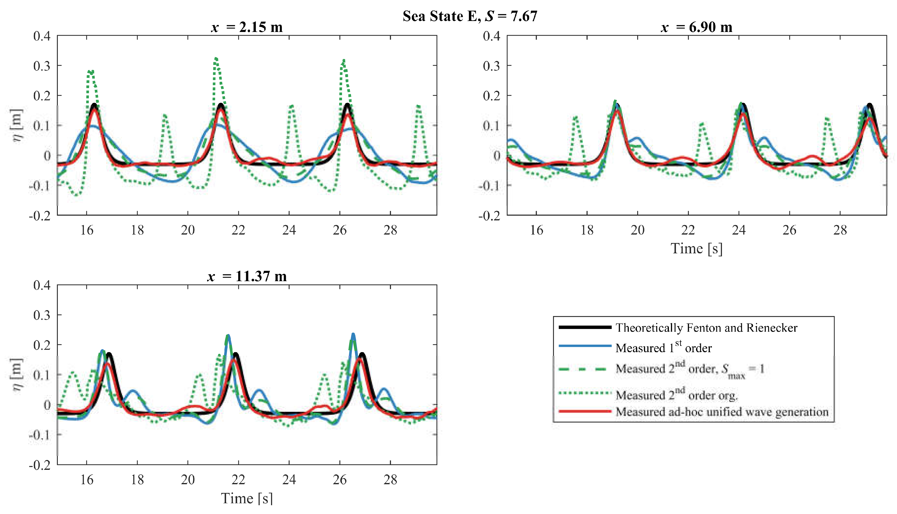
Results for Sea State E is shown in Figure 9. For that case second-order wavemaker theory generates too large waves in x = 2.15 m and a secondary wave is also seen in the wave trough of the primary wave. The first-order wavemaker theory is significantly better than the second-order wavemaker theory as no secondary waves are seen in x = 2.15 m. As in Figure 8, the waves generated by second-order wavemaker theory are breaking during the tests, which is the reason for the large wave crest are not observed for the two other locations in the figure. The modified second-order wavemaker theory is slightly better than the first-order wavemaker theory, but they are both far from the theoretical profile. The ad-hoc unified wave generation is a close match to the theoretical profile except for small deviations in the trough, but this is most likely due to reflections from the passive absorber in the wave flume.

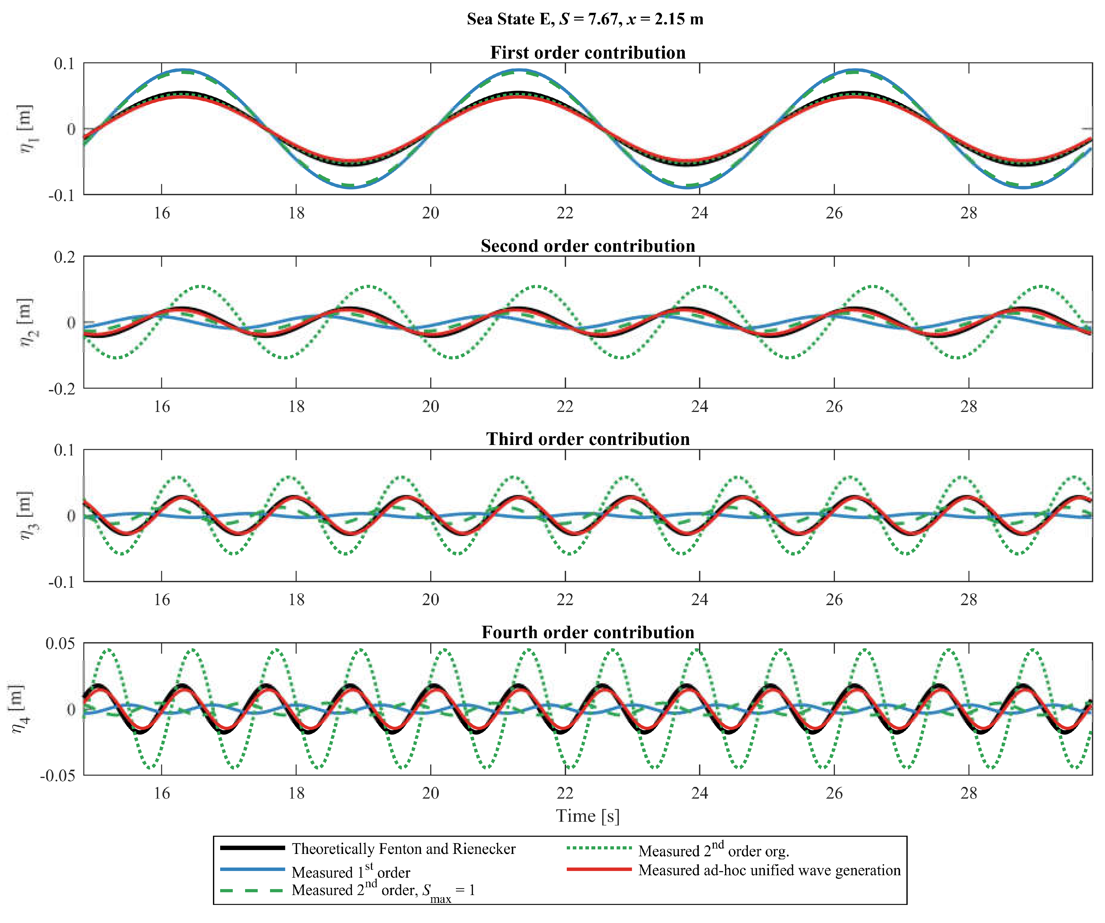
A more detailed analysis of the measured waves for Sea State E is shown in Figure 10 for x = 2.15 m. The time series of the primary and the first three superharmonics is calculated by Fourier transformation on the discrete frequencies nω. Thus, the measured components can be compared with the theoretical stream function wave components. The figure shows that the original second-order wavemaker theory generates higher harmonics that are significantly higher than the theoretical stream function wave. It also shows that only the ad-hoc method generates the correct amplitudes of the different contributions. Furthermore, a phase shift between the superharmonics and the first-order component is observed especially for the first-order generation method and the original second-order method. This phase shift demonstrates significant free energy to be present. Only the ad-hoc method has correct amplitudes and phases for all components.

It has been shown that first-order wavemaker theory can be used for S ≤ 0.8 and that the modified second-order wavemaker theory gives identical results as the second-order theory by Schäffer [3] when the second-order theory is valid. However, the modified second-order method performs significantly better when used outside the validity area. This is due to a more realistic value of the amplitude for the second-order harmonic, which for the method by Schäffer [3] has no upper limit and for the present tests is calculated to approximately two times the first-order amplitude in the worst case (Sea State E). In that case, the higher order harmonics have a significant influence, and therefore second-order theory is not valid for this case. This is shown in Figure 10 by comparing the contributions of the first four harmonics with the theoretical amplitudes. The second-order wavemaker theory can be used for S ≤ 1.5 with reasonable results. The ad-hoc unified generation can be used for all the tested conditions (tested up to S = 7.7).

6. Irregular Wave Results

The performance of the different wavemaker methods for the irregular waves are compared with the results from the COULWAVE model at different distances from the wavemaker. The measured surface elevations are shown for a time window including the highest wave.

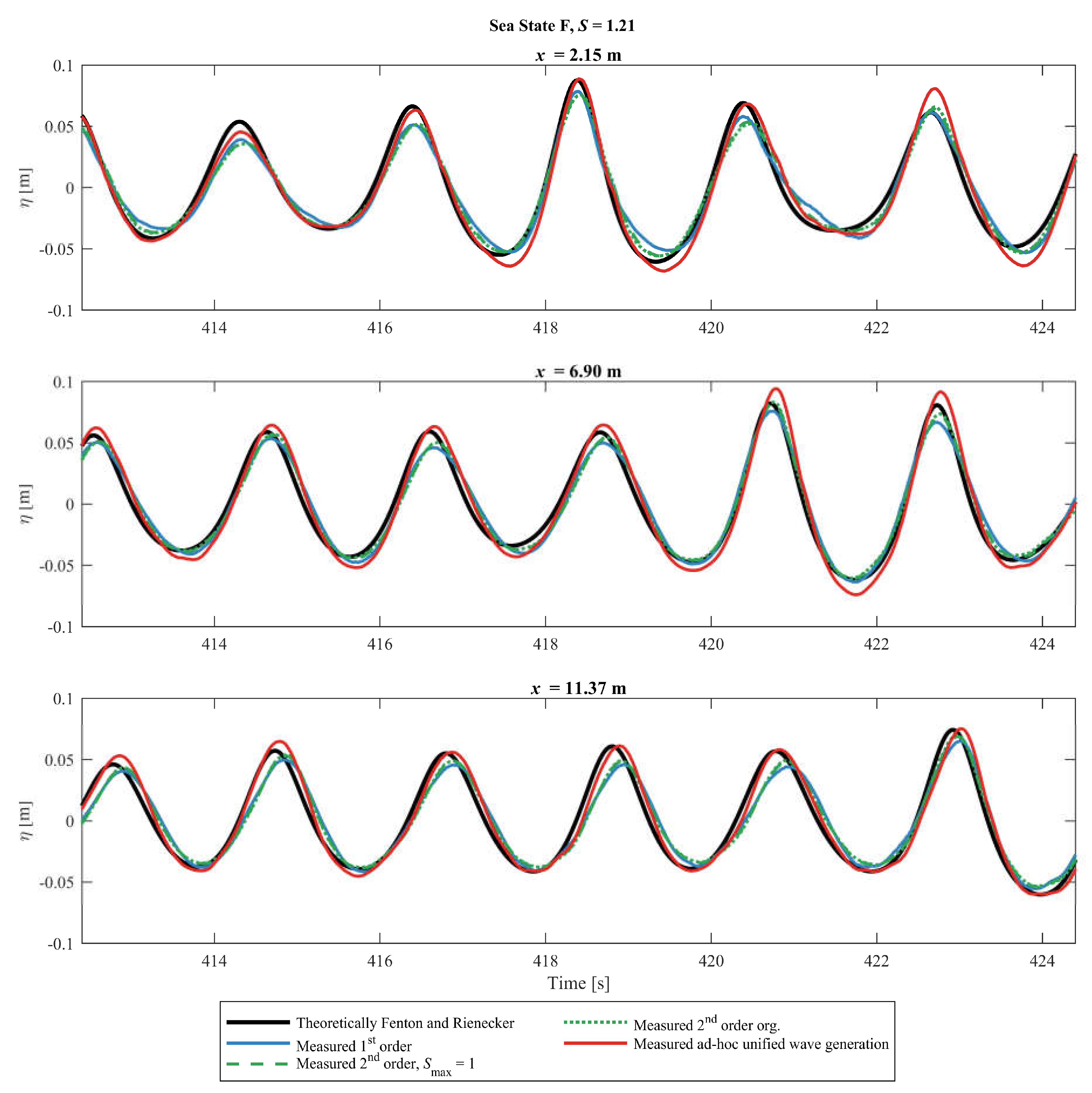
Results for Sea State F are given in Figure 11. The first and second-order wavemaker theories are according to the Le Méhauté diagram not expected to be valid for this sea state. Furthermore, the test is also outside the applicability range given by Schäffer [3]. However, the figure shows that all the tested methods give similar results and that they are a close match to the COULWAVE model with only minor deviations.

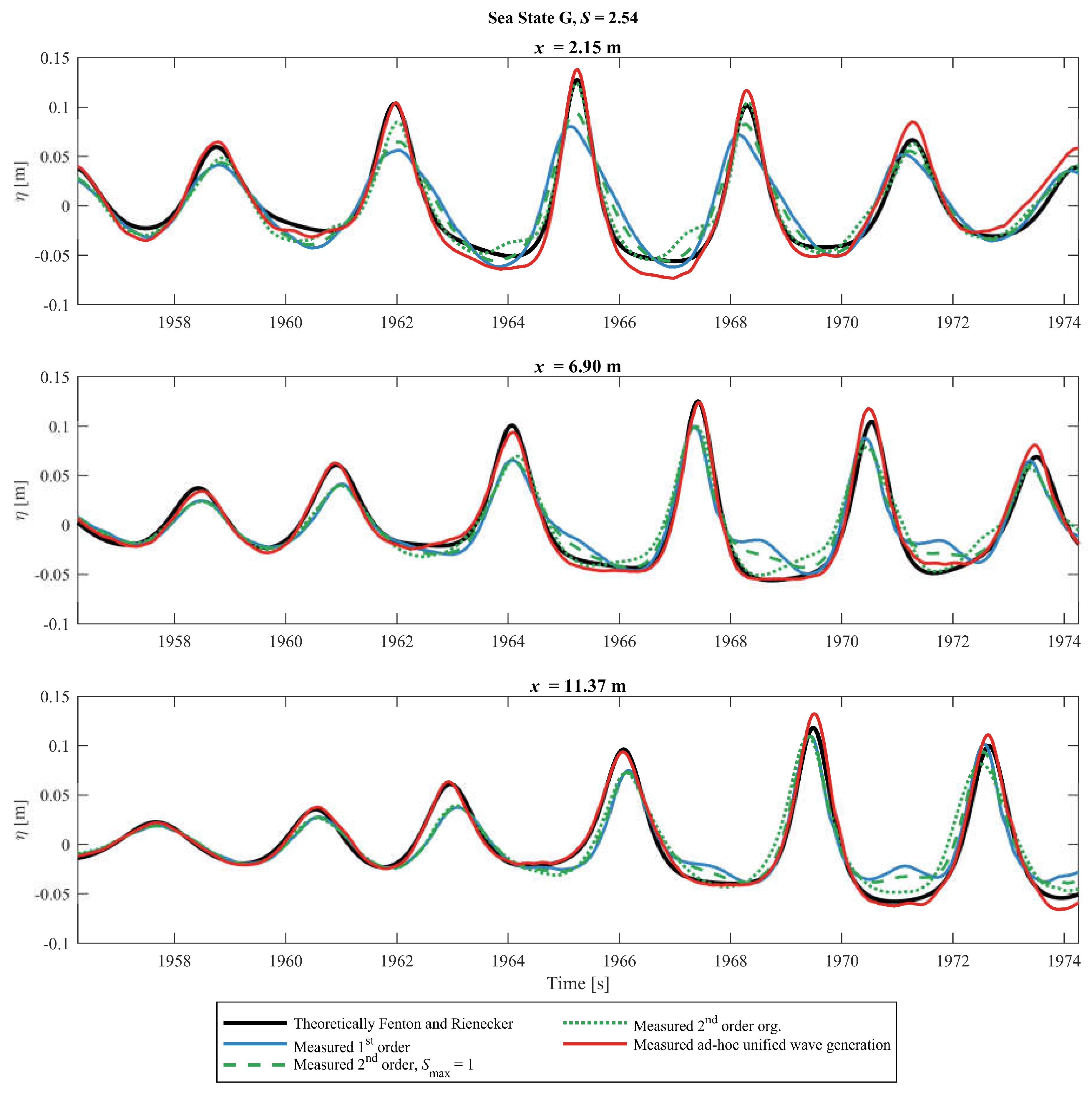
Figure 12 presents the results for Sea State G. For this case is the wave crest of the largest wave with the first-order wavemaker theory significantly smaller than the theoretical wave profile at x = 2.15 m. The original second-order wavemaker theory is closer to the numerical profile except for some deviations in the wave trough for x = 2.15 m. For the three wave gauges, it can be seen that the wave crest is too small for the largest waves when the waves are generated with the modified second-order wavemaker method, but except for that, it is a close match. The shape of the waves generated by the ad-hoc unified generation method is a close match but with a deeper wave trough at x = 2.15 m, but this is likely due to long reflected waves as it is not seen for the two other gauges.

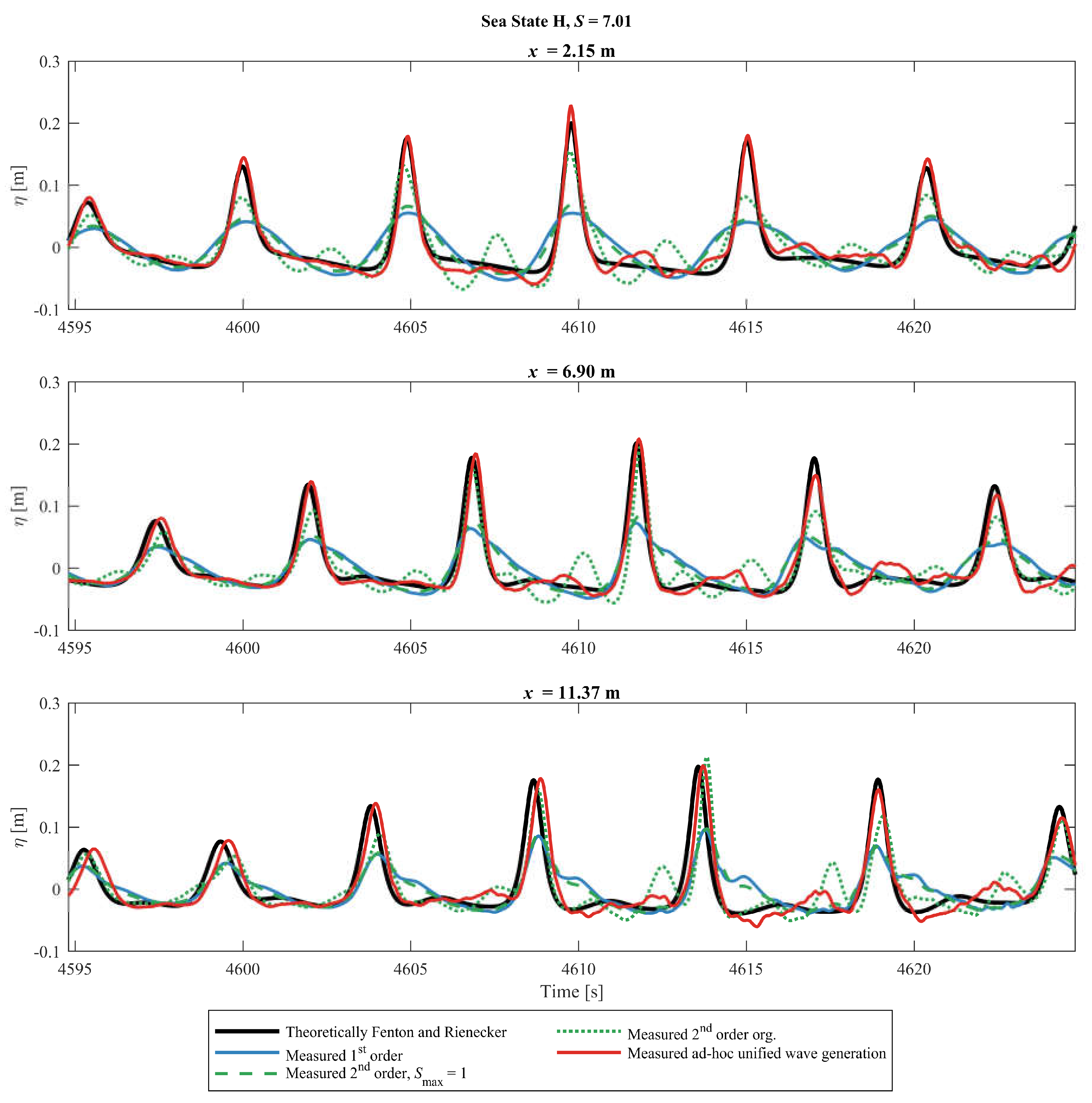
For Sea State H, the first-order wavemaker theory is deviating significantly from the numerical profile as the wave trough is not flat and long and the wave crest is not high and narrow, cf. Figure 13. The wave profile generated by the first-order wavemaker theory has a step front followed by a gentler rear as the waves propagate away from the wavemaker—this is due to the free and bound waves having different celerity. For x = 11.37, the free and bound waves are phase shifted to such a degree that the crest of both the free and the bound waves are visible. The second-order wavemaker method has a secondary crest in the wave trough, which is reduced significantly with the modified second-order method. The wave crest with the modified second-order wavemaker method is though significantly smaller than the theoretical but is still closer to the theoretical compared to the first-order wavemaker method. The modified method is better than the original second-order method as less free energy is generated, but for this case the amount of secondary energy is also much smaller than the target. The ad-hoc unified wavemaker method provides a close match to the numerical profile with only minor deviations, and for this sea state, only this method leads to acceptable results.

For irregular waves, the present tests showed that first-order wavemaker theory can be used for S ≤ 1.2, while the second-order wavemaker theory can be used for S ≤ 2 with reasonable results. The ad-hoc unified generation showed good performance and can be used for all the tested conditions (tested up to S = 7.0).

7. Conclusions

Model tests have been performed with the purpose to generate waves of various nonlinearity and evaluate different wavemaker methods. First-order, second-order and ad-hoc unified generation methods have been tested, and the validity range of each method has been found by physical experiments. Furthermore, a modification to the second-order wavemaker method was proposed to increase the validity to more nonlinear waves. The ad-hoc unified generation method for the regular waves was the most accurate wavemaker method, and if possible, it should be used, otherwise the modified second-order is preferable. For the irregular waves, the ad-hoc unified generation method is also the most accurate one, but it is also much more time-consuming in synthesize the signals. This is because a time series has to be prepared by a numerical model before waves can be generated in the physical model. Therefore, it is recommended to use the modified second-order wavemaker theory when it is valid.

Table 2. Applicability of each tested wavemaker method.

	Regular Waves				Irregular Waves
	First-order	Second-order	Modified second-order	Ad-hoc unified	First-order	Second-order	Modified second-order	Ad-hoc unified
S	0.8	1.5	1.5	∞	1.2	2.0	2.0	∞

summarizes the applicability ranges of each wavemaker method. For the regular waves, acceptable results are found with first-order wavemaker when S < 0.8, while second-order methods extends the validity to S < 1.5. The ad-hoc method is applicable for all the tested conditions (S < 7.7), but is expected to be reliable for all S values. For the irregular waves, acceptable results are found with first-order theory when S < 1.2. For both second-order methods acceptable results for irregular waves were found when S < 2.0. The ad-hoc method showed also for irregular waves good results for all the tested conditions. As it has not been possible to test all possible sea states these results should be taken as preliminary, but can be used until more tests have been performed.