Iterative Frequency-Domain Response of Floating Offshore Wind Turbines with Parametric Drag

Abstract

Methods for coupled aero-hydro-servo-elastic time-domain simulations of Floating Offshore Wind Turbines (FOWTs) have been successfully developed. One of the present challenges is a realistic approximation of the viscous drag of the wetted members of the floating platform. This paper presents a method for an iterative response calculation with a reduced-order frequency-domain model. It has heave plate drag coefficients, which are parameterized functions of literature data. The reduced-order model does not represent more than the most relevant effects on the FOWT system dynamics. It includes first-order and second-order wave forces, coupled with the wind turbine structural dynamics, aerodynamics and control system dynamics. So far, the viscous drag coefficients are usually defined as constants, independent of the load cases. With the computationally efficient frequency-domain model, it is possible to iterate the drag, such that it fits to the obtained amplitudes of oscillation of the different members. The results show that the drag coefficients vary significantly across operational load conditions. The viscous drag coefficients converge quickly and the method is applicable for concept-level design studies of FOWTs with load case-dependent drag.

1. Introduction

Research on floating instead of fixed-bottom offshore wind energy started more than ten years ago. Numerous demonstration projects with commercial-scale wind turbines have proven the feasibility of harvesting offshore wind energy at water depths beyond the limits of substructures rigidly connected to the seabed [1].

1.1. Coupled Aero-Hydro-Servo-Elastic Dynamics

For a prediction of the dynamic behavior of a Floating Offshore Wind Turbine (FOWT), a multidisciplinary analysis is necessary. There are different coupling effects between the submodels of aerodynamics, hydrodynamics, servodynamics and structural dynamics. This results from the soft substructure restoring forces, especially of semi-submersible concepts, leading to a slow fore-aft motion of the rotor and therefore an influence on the aerodynamics. One important example for the dynamic coupling effects is the influence of the wind turbine blade pitch controller on the global fore-aft mode of the FOWT. The controller pitches the blades, due to a change of the relative wind speed seen by the rotor, originated from a fore-aft oscillation of the platform. This pitching reduces the thrust and can eventually yield a fore-aft system instability as shown by [2,3,4], among others. The effect was experimentally shown for the semi-submersible FOWT concept of this work in [5]. Several open-source and commercial integrated FOWT models, respecting these couplings, have been developed. The first was the FAST model by National Renewable Energy Laboratory, Boulder, CO, USA (NREL) (see [6]).

Higher-fidelity models are necessary to model the impact the fore-aft motion of the rotor has on the inflow, the wake and the local flow around the airfoils. These unsteady aerodynamic effects have been investigated first by [7,8]. Experimental approaches followed by [9,10]. Various high-fidelity simulations have been performed, i.e., [11,12,13,14,15,16,17]. They show that these unsteady aerodynamic effects of the wake depend largely on the frequency and the amplitude of the fore-aft motion but also on the Tip Speed Ratio (TSR) of the rotor.

The common methodology for hydrodynamic FOWT simulations is a time-domain formulation, which respects the frequency-dependence of the hydrodynamic coefficients, derived from panel codes [18,19]. In the time-domain, the frequency-dependence results in a convolution integral, representing fluid memory effects (see Cummins’ equation [20]). Viscous effects are usually accounted for through the inclusion of the quadratic drag term of Morison’s equation [21]. This drag results on the one side in an excitation force, due to the wave particle motion, next to the Froude–Krylov and diffraction pressures from the panel code computation. On the other side, Morison drag results in a viscous damping of the floating body. Simplified models have been published neglecting the excitation part, modeling only the damping [22].

1.2. Hydrodynamic Viscous Drag

A common practice for the determination of the damping properties is to identify a linear damping matrix or quadratic generalized platform damping from model tests, such as in [22,23]. Another way is to identify the member-based Morison drag coefficients, instead of the lumped, generalized damping coefficients, see [24,25] or [26]. Commonly, free-decay tests are used to obtain these drag or damping coefficients from model tests. Computational Fluid Dynamics (CFD) simulations have also been used for the identification of FOWT drag [27].

As for the load case simulations in the seminal Offshore Code Comparison Collaboration (OC3) through Offshore Code Comparison Continuation, Continued, with Correlation (OC5) projects, the damping properties are usually estimated based on a calculation of the Reynolds number for different sea-states and a fixed platform. The obtained drag coefficients are then used equally for all load conditions in the participating tools.

The present study addresses the question of the load-case dependence of the drag coefficients for FOWTs. As we showed experimentally in [28], the viscous damping properties of FOWTs can vary significantly, depending on the load case. This is due to the strong Reynolds dependence ($\mathit{Re}=\widehat{v}D/\nu$, with velocity amplitude $\widehat{v}$, characteristic length D and kinematic viscosity $\nu$) and also a dependence on the Keulegan–Carpenter number (KC) ($\mathit{KC}=\widehat{v}T/D$, with period of oscillation T) of the drag coefficients, see ([29], Chapter 7) and, additionally, the body surface roughness [30]. For circular cylinders, the Reynolds and KC-dependence of the drag is given by Sumer and Fredsøe ([31], p. 144). It can be seen in that reference that the drag is a complex, not monotonous function of both nondimensional numbers. Therefore, generally reasonable values, only dependent on the roughness, are given in ([30], p. 117). For plates with sharp edges (like heave plates of semi-submersible FOWTs), it is different: here, flow separation is almost always present and the drag is independent of the Reynolds number. Thus, a parameterization is well possible. In [32], a monotonically decaying drag as function of KC is identified. KC is a function of the body diameter, the motion velocity amplitude and the period of oscillation. Thus, the heave plate drag is a function of the dynamic response of the FOWT. The drag values of [32] could be confirmed for FOWT model tests in [28] for the public TripleSpar design [33], which will be used in this work.

This dependence of the drag on the motion response makes it difficult to determine their magnitude a priori. The response would have to be obtained with an initial guess of the drag coefficients and be updated subsequently, based on the obtained response. Simulation times of common coupled FOWT models are approximately half the simulated time, which yields a large computational effort with such an iterative procedure.

Linear frequency-domain methods are therefore more appropriate for an iterative solution of the drag coefficients. Methods for the linearization of the quadratic drag are available, i.e., [34]. A simplified approach for FOWTs was presented recently by Pegalajar-Jurado et al. [35]. It accounts for the relative velocity between the body and the fluid. A more complex method for an iterative drag linearization for offshore structures in the frequency-domain was published by Langley in [36]. It was applied to FOWTs by Lupton [37]. The KC-dependence is not a subject of the latter publication as they focus on the linearization itself. The influence of the wind turbine aerodynamics on the response was also not considered.

The motivation of this work is to include all relevant aero-hydro-servo-elastic effects in a coupled dynamic frequency-domain model for an iterative solution of the response with a parameterized heave plate drag as function of KC. For this end, a generalized model for the member-based Morison viscous drag coefficients will be defined in Section 2. Subsequently, the linearized drag is obtained from the quadratic viscous drag. A reduced-order coupled model will be used to obtain the global system response. The results of Section 3 show the iteratively obtained heave plate drag coefficients and the global response predicted by the reduced-order model together with the one predicted by FAST [38], followed by the conclusions in Section 4.

2. Numerical Simulation Methods

This section starts with a description of the reference FOWT model used in this work. The hydrodynamic viscous drag model and its linearization will be addressed afterwards and subsequently its integration into a coupled low-order simulation model.

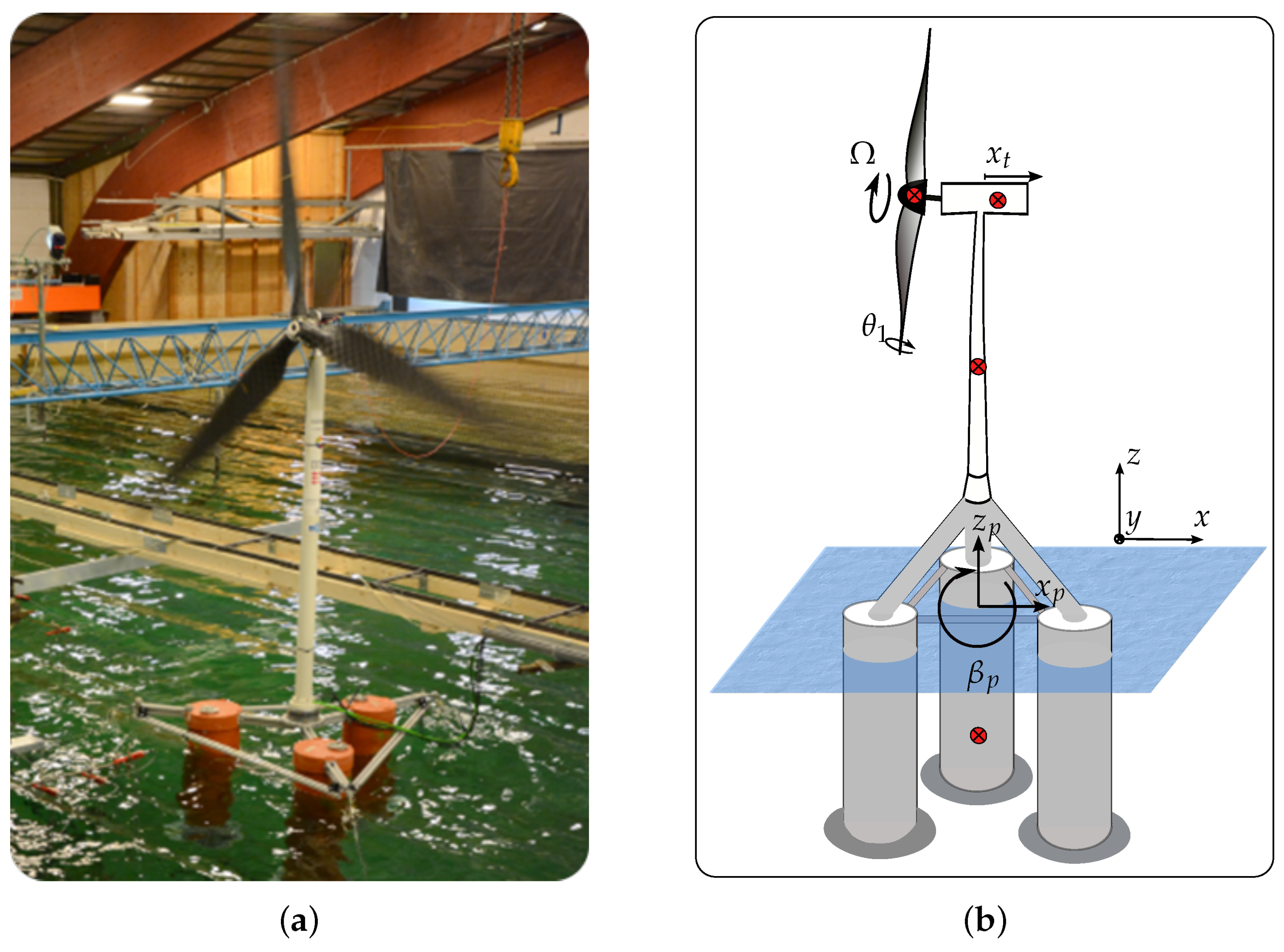
2.1. Reference Design

The FOWT design “TripleSpar” is shown in Figure 1. The left part of the figure shows an image of the scaled model of [39], which will be used in this paper, next to the full-scale prototype. The right part of Figure 1 shows the coupled simulation model, which will be introduced in Section 2.

The design was initially developed in the project INNWIND.EU [40]. It is a concept design for the research community and can be downloaded [41]. The main parameters can be found in

Table 1. TripleSpar Platform Main Properties.

Platform draft [m]	54.5	Number of mooring lines	3	Rated rotor speed [rpm]	9.6
Platform column radius [m]	7.5	Mooring line length [m]	610.0	Rotor diameter [m]	178.3
Platform column spacing (to centerline) [m]	26.0	Water depth [m]	180.0	Turbine mass [${10}^6$ kg] (incl. tower)	1.1
Platform mass [${10}^6$ kg]	28.3	Rated wind speed [$\mathrm{m}/\mathrm{s}$]	11.4	Hub height [m]	119.0

. It is a deep-drafted semi-submersible with a large portion of the hydrostatic restoring coming from the low center of mass. While the columns are made from pre-stressed concrete, the thin heave plates at the lower ends of the columns are made out of steel. Although it has slender columns, it has a lower draft than a spar, due to the three columns. Spars and semi-submersibles with heave plates are common FOWT substructures today [1], which makes this concept well suited for the presented research.

The experimental model was tested in a scale of 1:60 in 2016 at the Danish Hydraulic Institute (DHI) with results presented in [5,28,39]. The test program included irregular wave with wind Load Cases (LCs) with different significant wave heights $H_s$ and peak spectral periods $T_p$. Two of these cases are considered in the present work, LC 7 ($H_s=5.5$ m and $T_p=8.4$ s) and LC 9 ($H_s=9.5$ m and $T_p=11.1$ s).

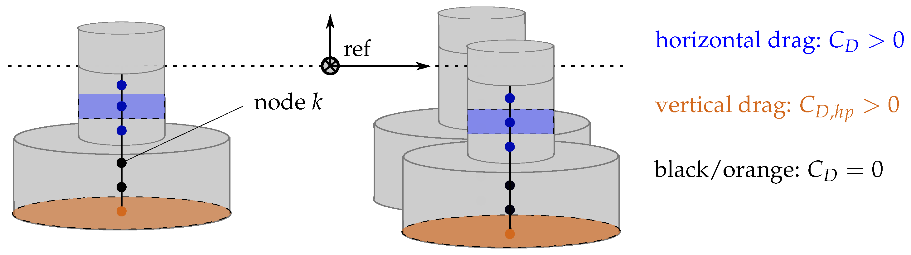
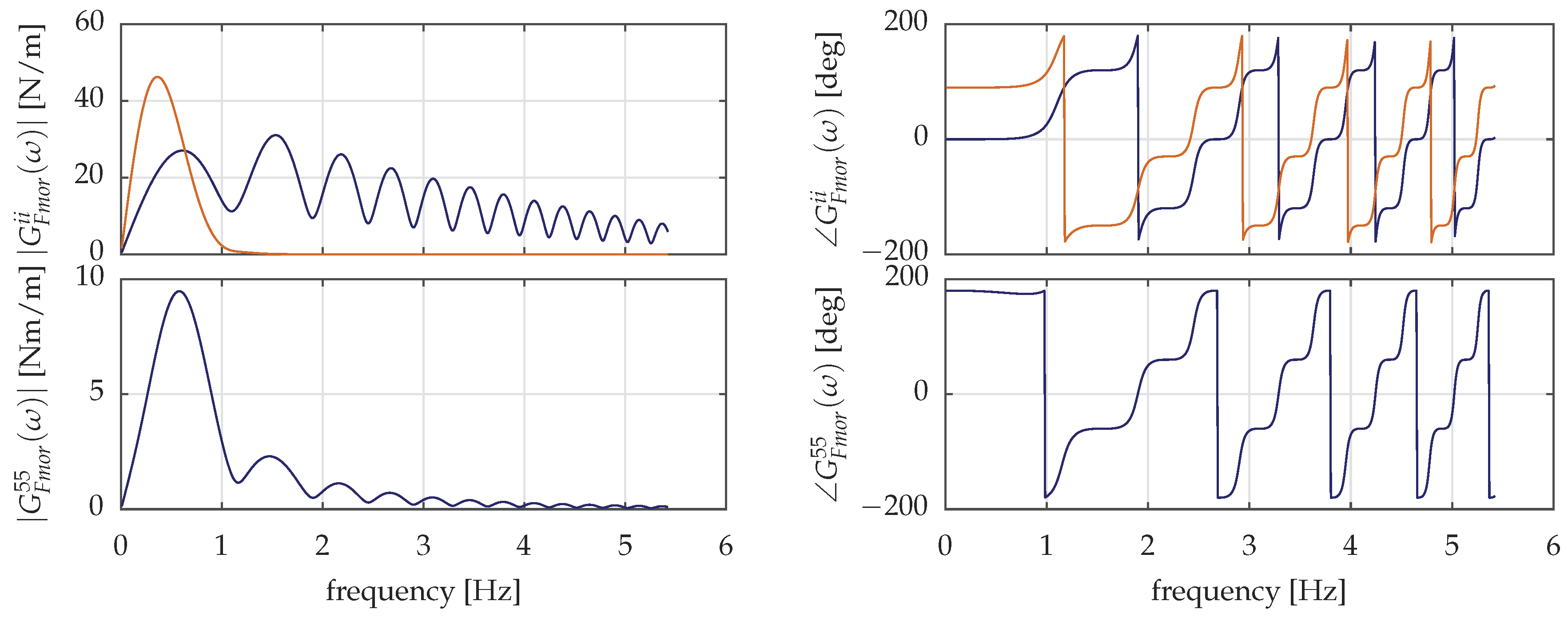
2.2. Generalized Morison’s Equation

Morison’s original formulation [21] was extended for the present work to account, firstly, for the relative fluid velocity due to the body motion and secondly, for heave plates with force components in vertical direction (in the body-fixed frame). The substructure is discretized through nodes as shown in Figure 2. For a flexible model setup, each node k has modified Morison coefficients $C_{D,i}^{\ast }$ for all three directions i with the area $A_{ik}$, projected on direction i in body-fixed coordinates (attention needs to be paid to vertical drag coefficients for heave plates $C_{D,z}=C_{D,\mathit{hp}}$. Here, the drag force is calculated as $F_{D,z}=C_{D,z}^{\ast }{v}_z^2$, whereas, in HydroDyn [42], it is assumed that for each heave plate a node is defined for both ends and half the drag force applies to each end).

The viscous drag term of Morison’s equation is

$$F_{D,\mathit{ik}}=C_{D,ik}^{\ast }\left(v_{w,ik}-v_{b,ik}\right)|v_{w,ik}-v_{b,ik}|$$

(1)

with the modified hydrodynamic coefficients

$$C_{D,ik}^{\ast }=\frac{1}{2}{\rho }_w{A}_{ik}{C}_{D,ik}$$

(2)

The nodal body velocities $v_{b,ik}$ are a function of the generalized coordinates, shown in Figure 1. The wave particle velocities $v_{w,ik}$ can be calculated in the frequency-domain using deepwater approximation with linear potential flow theory [18], giving $v_{w,x}(\omega ,z)=\zeta \left(\omega \right){\mathrm{e}}^{kz}$ with the wave number k, the upward vertical coordinate z at Still Water Level (SWL) and the wave height amplitude spectrum $\zeta \left(\omega \right)$. The substructure has transverse drag forces in horizontal direction only for the slender columns, not for the heave plates.

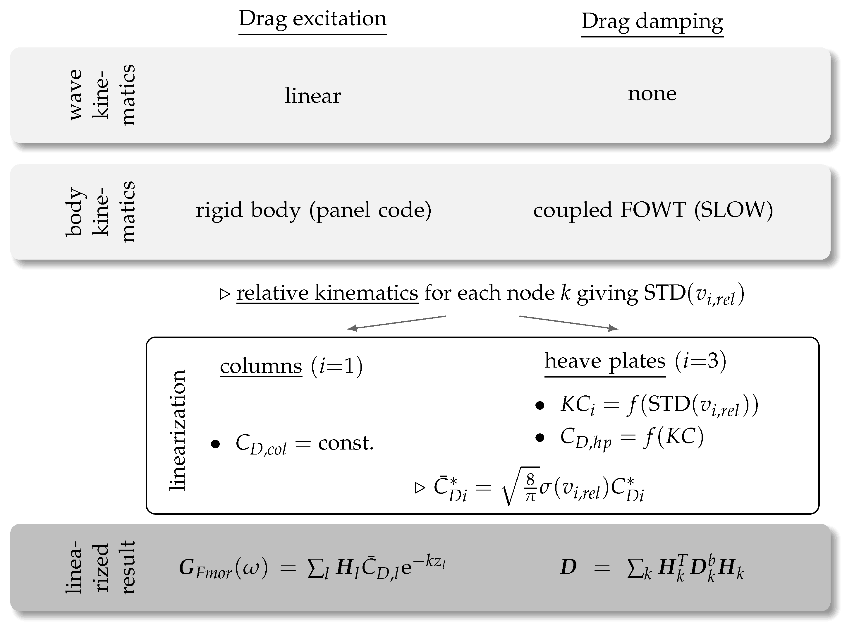
2.3. Linearized Viscous Drag Model

A linearized description of the drag is necessary for the iterative frequency-domain solution. Morison’s drag term, Equation (1), contains both damping and excitation forces due to the relative velocity between the undisturbed fluid and the body. The next sections address first the method to obtain the linearized drag coefficients. Thereafter, both the calculation of the excitation part through a transfer function from the wave height to the nodal forces follows as well as the nodal damping of the FOWT platform will be addressed.

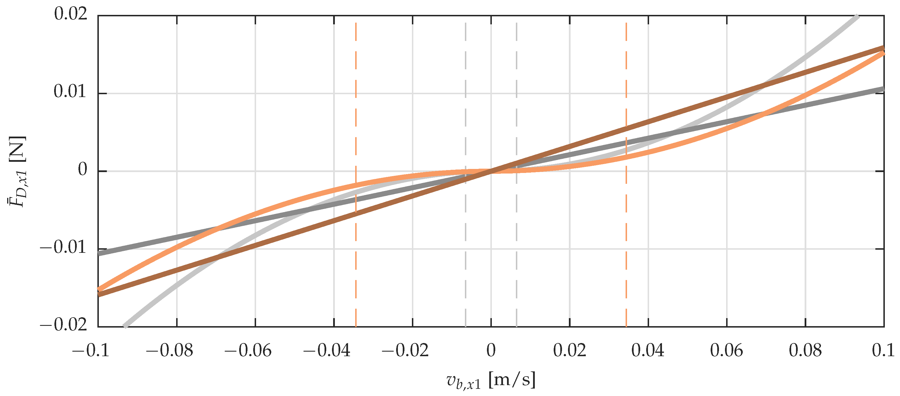
2.3.1. Drag Linearization

Possible linearization methods for Equation (1) are harmonic or stochastic linearization. In the case of harmonic linearization, the error due to neglected higher-order terms is minimized for a sinusoidal velocity time series. Stochastic linearization methods improve the linearized model quality for stochastic velocity time series. A discussion with a comparison of alternatives can be found in [43].

The stochastic linearization used here follows Borgman [34]. It is based on the Standard Deviation (STD) of the relative fluid velocity. In this work, an efficient method for the linearization of the velocity-dependent part of Equation (1) is chosen: the nonlinear drag coefficient $C_{D,ik}$ is split into one part dependent on the wave-velocity and a part dependent on the body-velocity. A comparable approach was selected by Pegalajar-Jurado et al. [35]. The linearized nodal Morison force ${\overline{F}}_{D,\mathit{ik}}$ results with the approximation as

$${\overline{F}}_{D,\mathit{ik}}={\overline{C}}_{D,ik}^{w\ast }{v}_{w,ik}-{\overline{C}}_{D,ik}^{b\ast }{v}_{b,ik}$$

(3)

in direction i. The part representing the external drag-excitation is (${\overline{C}}_{D,ik}^{w\ast }{v}_{w,ik}$), and the damping part is ($-{\overline{C}}_{D,ik}^{b\ast }{v}_{b,ik}$). Only the latter part was considered in [35], while the former was neglected. The approach selected here with Equation (3) neglects the cross-correlation between fluid and body velocity. However, this cross-correlation can be considered when calculating the linearized counterpart ${\overline{C}}_{D,ik}$ of the nonlinear drag coefficients $C_{D,ik}$.

The linearized drag coefficients ${\overline{C}}_{D,ik}$ for wave and body velocities are, following [34], a function of the STD $\sigma \left(v_{ik}\right)$ of the velocity in direction i of a node k with characteristic cross-sectional area $A_{ik}$, normal to direction i as

$${\overline{C}}_{D,ik}^{\ast }=\sqrt{\frac{8}{\pi }}\sigma (v_{w,ik}-v_{b,ik})\frac{1}{2}{C}_{D,ik}^{\ast }$$

(4)

A challenge for the implementation of Equation (4) is related to the established coupled simulation method, described in the introduction. Commonly, the first-order wave forces and also the slow-drift forces are assumed to be independent of the body states. They are therefore calculated a priori and the forces are an external input to the simulation. For an iterative solution of Equation (4), this a priori calculation is not possible anymore. A modification of Equation (4) will therefore be made.

2.3.2. Drag Excitation

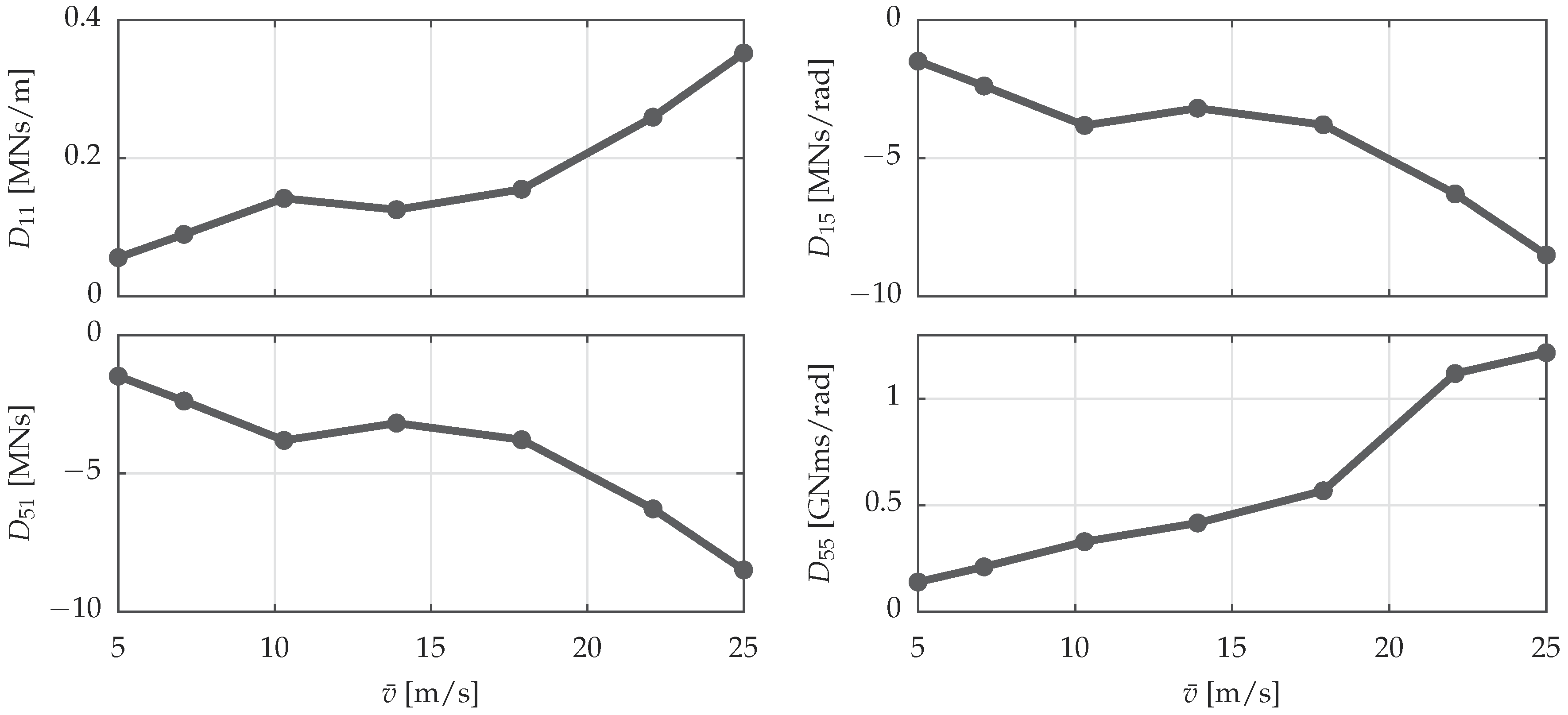
The external Morison excitation force can be written as a transfer function, when linearized. The goal is to obtain these transfer functions for the generalized platform coordinates $\mathit{\xi }$ (for the low-order coupled model, subject of Section 2.4, they are reduced to $\mathit{\xi }={[x_p,z_p,{\beta }_p]}^T$). With the wave particle velocities $v_w(\omega ,x,z)$, the transfer functions from the wave height ${\zeta }_0$ at the reference position to the three translational (superscript t) forces are

$${\mathit{G}}_{\mathit{Fmor}}^t\left(\omega \right)=\sum _{k=1}{\overline{C}}_{D,ik}^{w\ast }{v}_{w,ik}\left(\omega \right)\frac{1}{\widehat{\zeta }}$$

(5)

For the rotational direction (superscript r) from ${\zeta }_0$ to the three generalized moments on the platform about the platform reference point, here the Center of Flotation (CF) holds

$${\mathit{G}}_{\mathit{Fmor}}^r\left(\omega \right)=\sum _{k=1}{\mathit{r}}_k\times {\mathit{G}}_{\mathit{Fmor}}^t\left(\omega \right)$$

(6)

It is the cross product with the position vector ${\mathit{r}}_k$ to each node k. Equations (5) and (6) can be unified with the transformation tensor for the nodes ${\mathit{H}}_k$, assuming here a rigid platform, as

$${\mathit{H}}_k=\mathit{H}\left({\mathit{r}}_k\right)={\left[\begin{array}{cc}{\mathit{I}}^{3\times 3}& \tilde{\mathit{S}}\left({\mathit{r}}_k\right)\end{array}\right]}^T$$

(7)

The cross-product is written with the operator $\tilde{\mathit{S}}\left(\mathit{a}\right)\mathit{b}=\mathit{a}\times \mathit{b}$ and I denotes the identity matrix. Then,

$${\mathit{G}}_{\mathit{Fmor}}\left(\omega \right)=\sum _k{\mathit{H}}_k\mathrm{diag}({\overline{C}}_{D,i}^{w\ast })v_{w,k}\frac{1}{\widehat{\zeta }}$$

(8)

results. Figure 3 shows the obtained linear transfer functions for the TripleSpar. The calculation of the wave kinematics at the longitudinal column position results in the observed interference effect.

In order to keep the above-mentioned a priori calculation of the exciting forces, the generalized body velocity response spectrum for the calculation of $v_{b,ik}$, Equation (3) is calculated from the panel code Response Amplitude Operator (RAO) $\xi \left(\omega \right)/\zeta \left(\omega \right)$ and not from the coupled model of Section 2.4. This is convenient because the panel code calculation is performed as pre-processing of the coupled simulation. The RAO is differentiated to obtain the generalized velocity transfer function

$${\mathit{G}}_{\zeta \rightharpoondown \dot{\xi }}\left(j\omega \right)=j\omega \frac{\xi \left(\omega \right)}{\zeta \left(\omega \right)}.$$

(9)

The cross-spectral density matrix of the generalized platform velocities is

$${\mathit{S}}_{\dot{\xi }\dot{\xi }}\left(\omega \right)={\mathit{G}}_{\zeta \rightharpoondown \dot{\xi }}\left(\omega \right)S_{\zeta \zeta }{\mathit{G}}_{\zeta \rightharpoondown \dot{\xi }}^{\ast T}\left(\omega \right)$$

(10)

with the complex conjugate transpose ${\mathit{G}}^{\ast T}$. The velocity spectra ${\mathit{S}}_{v_k{v}_k}\left(\omega \right)$ of the nodes k of Figure 2 are obtained with the cross-spectral density matrix ${\mathit{S}}_{\dot{\xi }\dot{\xi }}\left(\omega \right)$ of the reference point. The nodal velocity cross-spectral density matrices ${\mathit{S}}_{v_k{v}_k}\left(\omega \right)\in {\mathbb{R}}^{(3\times 3)}$ of which holds ${\sigma }^2\left({\mathit{v}}_{b,k}\right)={\int }_0^{\infty }{\mathit{S}}_{v_k{v}_k}\left(\omega \right)\mathrm{d}\omega$, in translational directions become

$${\mathit{S}}_{v_k{v}_k}\left(\omega \right)={\mathit{H}}_k{\mathit{S}}_{\dot{\xi }\dot{\xi }}\left(\omega \right){\mathit{H}}_k^T.$$

(11)

As stated, the response spectra ${\mathit{S}}_{\dot{\xi }\dot{\xi }}$ result from the RAO, independent of the coupled system response. This approach yields a significant simplification of the computational implementation, while considering the relative fluid velocities instead of the absolute ones. The approach mainly respects relatively well the body response from first-order wave forces. It neglects, however, the low-frequency response at the platform eigenfrequencies and all wind turbine-related effects. This simplification can be seen as a separation of frequency ranges: the range of the platform eigenfrequencies and the one of the first-order waves. The discussed drag excitation forces act at the first-order wave frequencies, above the platform eigenfrequencies. Thus, neglecting the response at the platform eigenfrequencies is consistent, when looking only at the first-order wave frequencies. It is noted, however, that this frequency-domain perception is a simplification of the complex nonlinear flow phenomena in the time-domain.

For the TripleSpar design (Figure 1), it was found that the velocity-induced excitation of Equation (1) is small, about 20 times smaller than the acceleration-dependent Froude–Krylov forcing. The results of this study will be published in the PhD dissertation related to this work.

2.3.3. Drag Damping

In this section, the drag coefficients of Equation (3), related to the damping ${\overline{C}}_{D,ik}^{b\ast }$, will be identified. The damping is part of the system properties: in a unified state-space description of the FOWT, it is part of the system matrix (A) and influences the eigendynamics. These eigendynamics are especially important for the prediction of the system stability and for the controller design, as mentioned in the Introduction. Consequently, this coupling should be taken into account when determining the drag. To do this, an iteration is necessary: the hydrodynamic damping is updated as a function of the entire system response of the coupled model, until the calculation converges.

Figure 4 (left) shows the velocity STD over the 1:60 scaled TripleSpar columns of [39] for two sea states. The body velocity depends on the depth, in a way determined by the inherent wave response properties of the floater. The drag coefficient, Figure 4 (right), calculated with Equation (4), depends in the same way on the body velocity. The linearized nodal drag force ${\overline{F}}_{D,x1}$ for the upper node at SWL for one column is shown in Figure 5, together with the nonlinear drag force resulting from the nodal velocity $v_{b,x1}$. The figure shows ${\overline{F}}_{D,x1}$ for the same two environmental conditions as Figure 4. The linearization depends clearly on the response magnitude (STD, marked by dashed lines).

The calculation of the linearized drag coefficients ${\overline{C}}_{D,ik}^{b\ast }$ with Equation (4) for the damping problem is again simplified. In order to separate the a priori calculation of external forces, which is based on the undisturbed wave kinematics $v_{w,ik}$, from the simulation, the undisturbed wave kinematics are neglected for the damping problem. This approach is consistent with the above-mentioned separation of frequencies: the low-frequency response, for which the damping is of critical influence, is outside the first-order wave frequencies.

The obtained linear nodal drag coefficients ${\overline{C}}_{D,ik}^{b\ast }$ can be integrated giving a generalized coefficient matrix $\mathit{D}\in {\mathbb{R}}^{(6\times 6)}$ such that the generalized linearized Morison drag force ${\overline{\mathit{F}}}_D^b$ on the platform CF can be written as

$${\overline{\mathit{F}}}_D^b=\mathit{D}\dot{\mathit{\xi }}.$$

(12)

This is a very straightforward description, which can be used across models, i.e., to update the RAO with the viscous drag forces. The integration is again written using the transformation tensor $\mathit{H}\left({\mathit{r}}_k\right)$ of Equation (7)

$$\mathit{D}=\sum _{k=1}{\mathit{H}}^T\left({\mathit{r}}_k\right){\mathit{D}}_k^b\mathit{H}\left({\mathit{r}}_k\right)$$

(13)

with the damping matrix of the nodes

$${\mathit{D}}_k^b=\mathrm{diag}\left([{\overline{C}}_{D,\mathit{xk}}^b,{\overline{C}}_{D,\mathit{yk}}^b,{\overline{C}}_{D,\mathit{zk}}^b]\right).$$

(14)

The iteration and the obtained damping matrix D are shown in Figure 6 for the scaled TripleSpar. The solution converges already after about four iterations.

In order to assess the quality of the linearization of the damping problem, the overall Morison drag forces ${\mathit{F}}_D^b\left(t\right)$ were calculated for an LC of the scaled experiment [39]. The time series were calculated once with the quadratic drag force (Equation (1)) and once with the linearized drag force (Equation (3)). For a clear comparison, only the damping force is shown and the drag excitation part is set to zero. The left part of Figure 7 shows the generalized platform velocities. The right side shows the integrated generalized forces in the respective coordinates. The linearized drag is well in line with the nonlinear one, except for the larger peaks of the velocity. Here, the nonlinear model reaches larger values.

This completes the linear Morison model. The next section will introduce the low-order coupled simulation model.

2.4. Low-Order Aero-Hydro-Servo-Elastic Model

A mechanical sketch of the low-order coupled simulation model, which is used in this work, was shown in Figure 1. The model has been developed with the focus of a computationally efficient representation of the overall dynamics of the FOWT for control design and an overview on critical load situations. It was used in comparable configurations in previous works [4,44,45,46]. Its derivation starts with physical (as opposed to black-box) models, keeping the basic nonlinearities. In a next step, the nonlinear models are linearized. A frequency-domain computation of the response spectra will be used in the present work. The model will be called Simplified Low-OrderWind Turbine (SLOW) in the following.

The structural model is based on a flexible multibody formulation with rigid and flexible bodies according to [47,48]. For this work, the coupled equations of motion have been set up for six Degrees of Freedom (DoF) in 2D: the floating platform rigid body in surge ($x_p$), heave ($z_p$) and pitch (${\beta }_p$), a flexible tower with one representative coordinate $x_t$, the rotor speed $\mathsf{\Omega }$ and the blade pitch actuator ${\theta }_1$ (see Figure 1). These DOFs are selected in order to reduce the system to the most important effects, which are critical for the main system dynamics. These act usually in the direction of wind and waves (x). The main simplifications of the aerodynamics and hydrodynamics significantly accelerate the model execution, even in frequency-domain.

The hydrodynamic model includes first-order panel code coefficients and second-order slow-drift forces through Newman’s approximation. As in most FOWT simulators, wave drift damping, in the sense of ([30], p. 153), is not included. The radiation problem has been simplified through a frequency-independent added mass as in [49]. Radiation damping is completely neglected because it has negligible effects for the TripleSpar.

The physical modeling assumptions can be summarized as

● Structural dynamics:	6 DOFs, 2D motion,
● Aerodynamics:	Quasi-static, rotationally sampled turbulence,
● Hydrodynamics:	1st-order coefficients, Morison viscous drag, parametric heave plate drag, simplified radiation, 2nd-order slow-drift approximation,
● Mooring dynamics:	Quasi-static,
● Control:	Model-based Proportional-Integral (PI),
● Solution:	Time-domain & frequency-domain.

3. Results

The previously developed methods for modeling both the linearized wave excitation forces and the linearized damping forces from drag will now be coupled with a parametric function for the heave plate drag. The results are shown for environmental conditions used in the EU-project LIFES50+ for fatigue assessments ([50], Chapter 7). They are listed in

Table 2. Environmental Conditions for Operational Load Cases Extracted from [50], (Krieger, 2016), Chapter 7, with permission from DNV-GL, 2018.

Wind Speed $\overline{v}$	[m/s]	5.0	7.1	10.3	13.9	17.9	22.1	25
Significant Wave Height $H_s$	[m]	1.4	1.7	2.2	3.0	4.3	6.2	8.3
Peak Spectral Period $T_p$	[s]	7.0	8.0	8.0	9.5	10.0	12.5	12.0

.

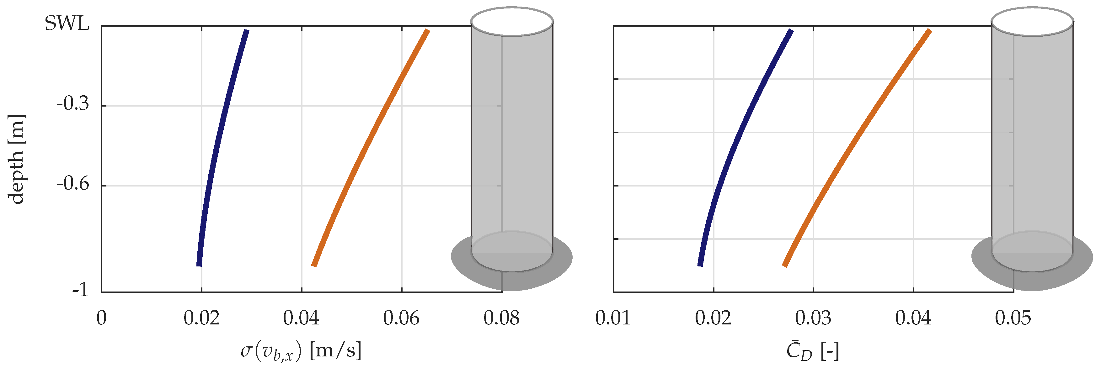
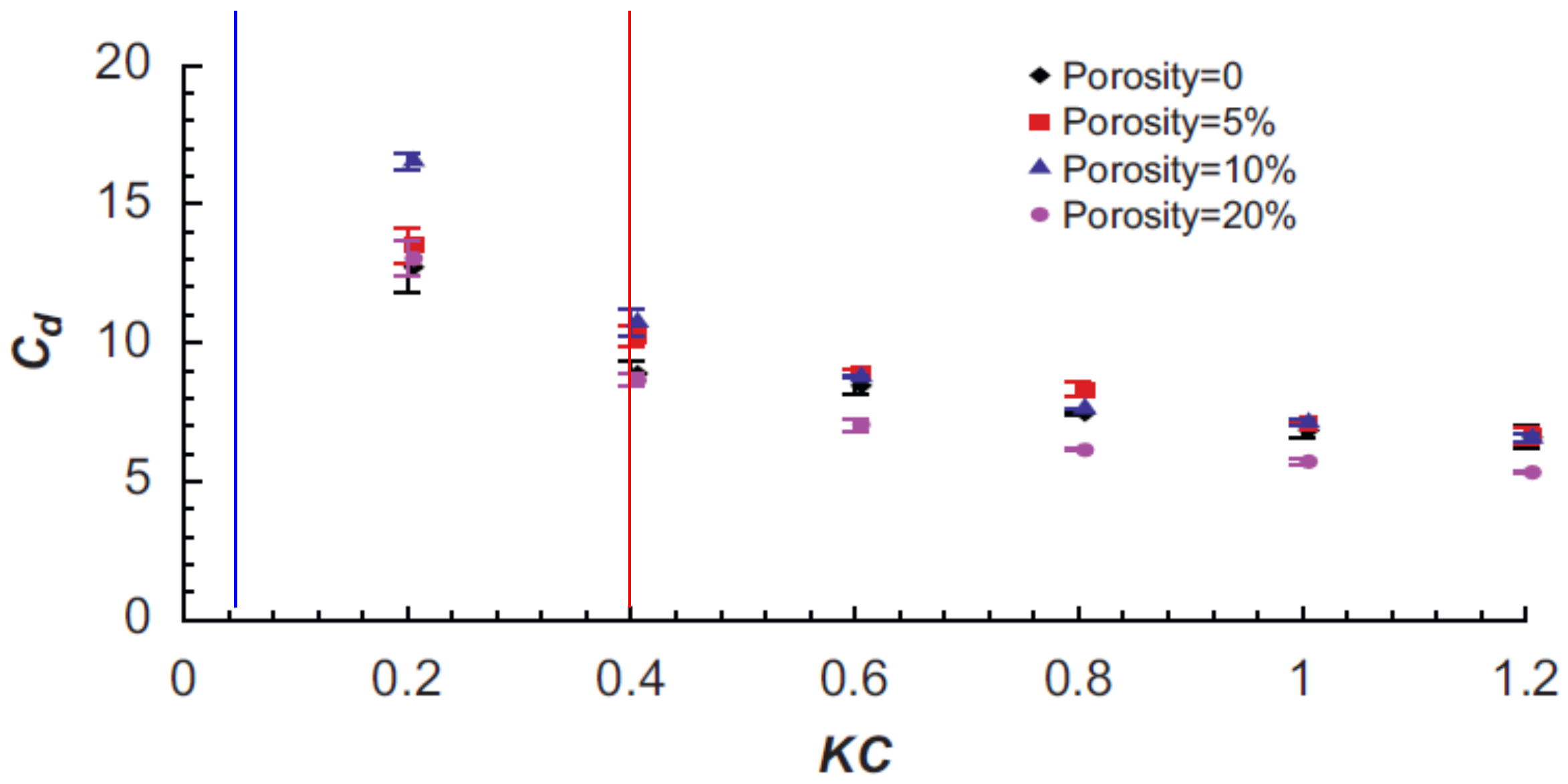
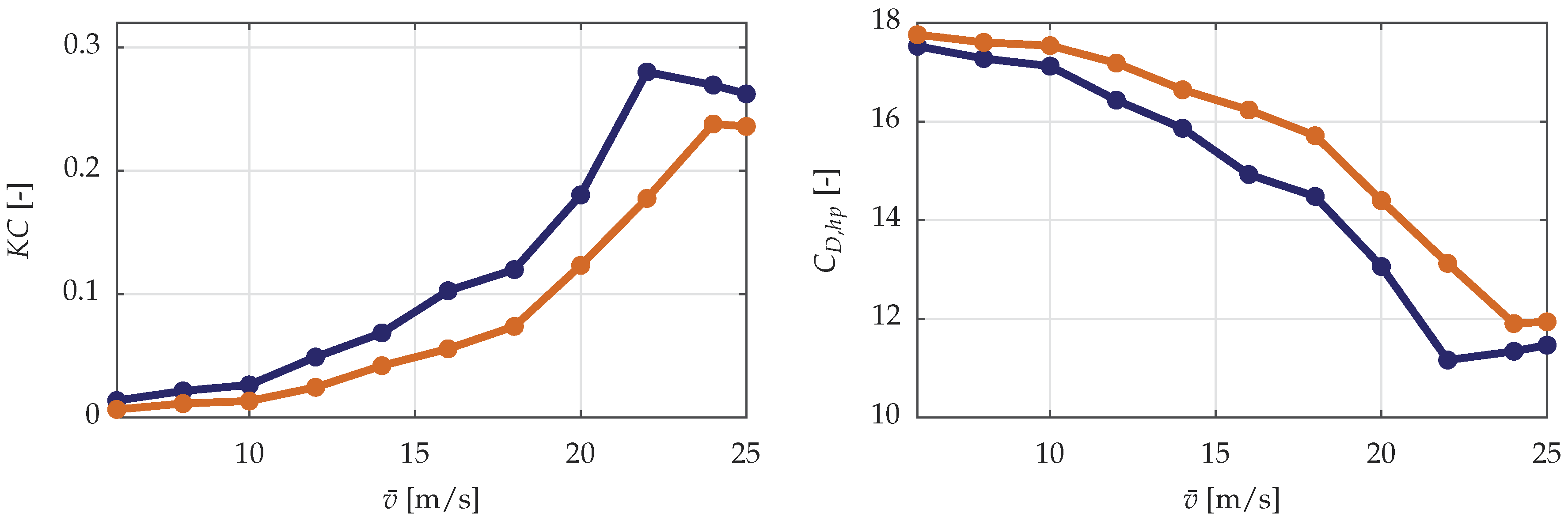
3.1. Parametric Drag

The parameterization of the column drag coefficients $C_{D,ik}$ is difficult due to their dependence on both Reynolds and KC-number, as described in the Introduction. In [28], the heave plate drag $C_{D,hp}$ was identified for coupled model tests of the TripleSpar, including the wind turbine and controller. The identified drag compares well with the values published by Tao et al. ([32], p. 1012). The authors of that publication identified the heave plate drag as a function of $\mathit{KC}$ as shown in Figure 8.

For this work, the values of Figure 8 were parameterized for an online interpolation, based on the instantaneous KC. Although the column drag $C_{D,ik}$ is not parameterized, the parameterization of the heave plate drag $C_{D,hp}$ improves the representation of the global FOWT dynamics. This is because the heave plate drag influences strongly the fore-aft dynamics of the rotor, which induce the couplings with aerodynamics and the controller, as described in the Introduction.

3.2. Solution Procedure

The computational implementation of the iterative hydrodynamic model is shown, as a summary of the previous sections, for the drag excitation forces and the damping forces in Figure 9. It visualizes the simplified representation of the relative fluid velocity between the wave particles and the body of Section 2.3. The procedure for the excitation problem focuses on the first-order wave frequencies, while the procedure for the damping problem focuses on the lower frequencies, at the platform eigenfrequencies.

The linearization is the same for the columns and the heave plates. The nonlinear drag coefficients of the heave plates, however, are parameterized and change, dependent on the member response magnitude.

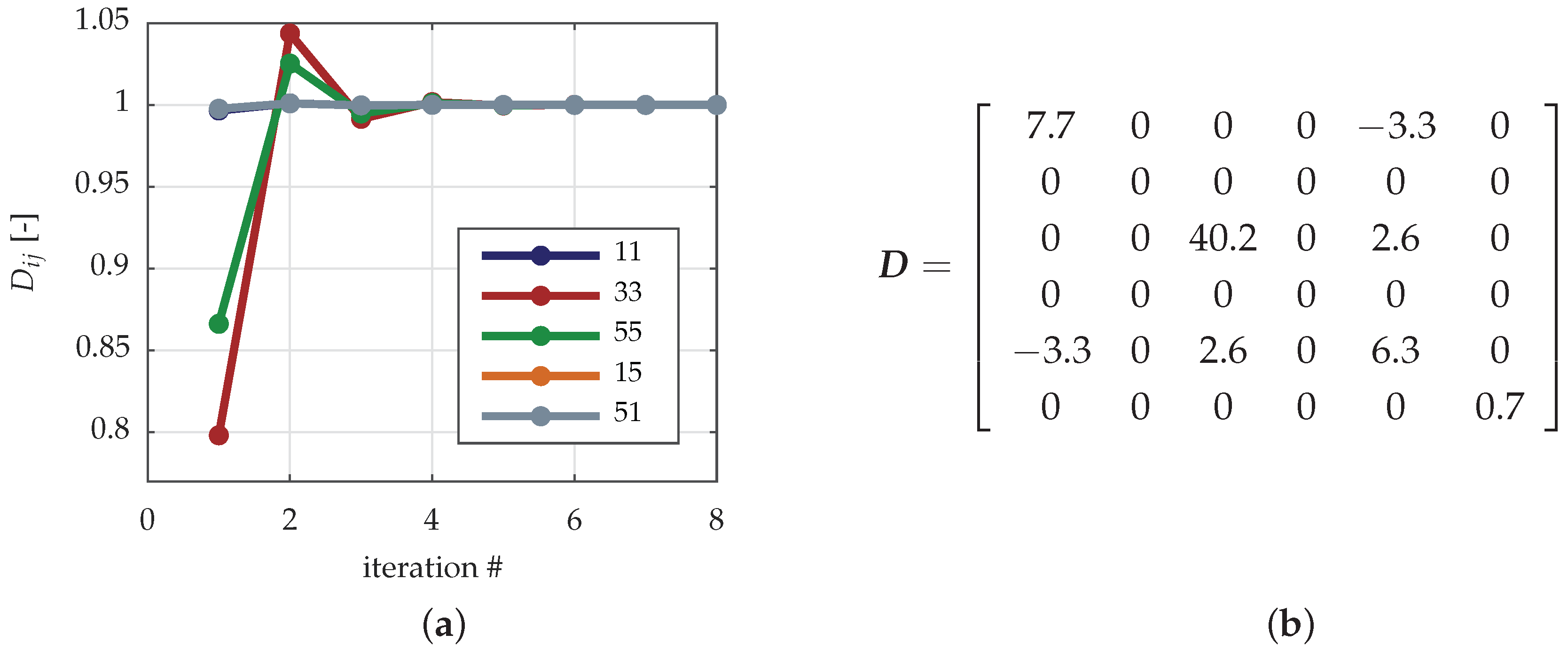
3.3. Iterative Solution

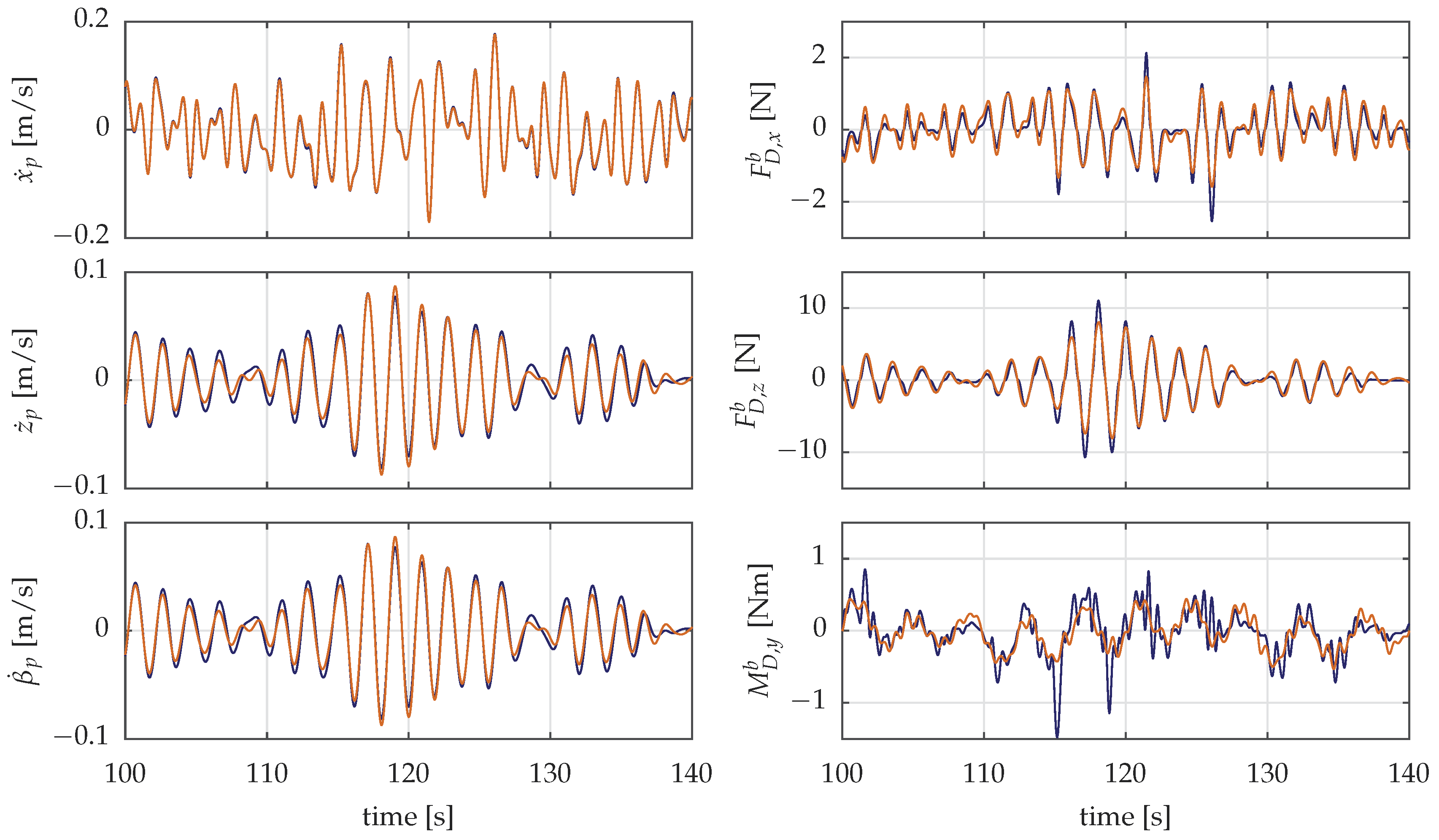
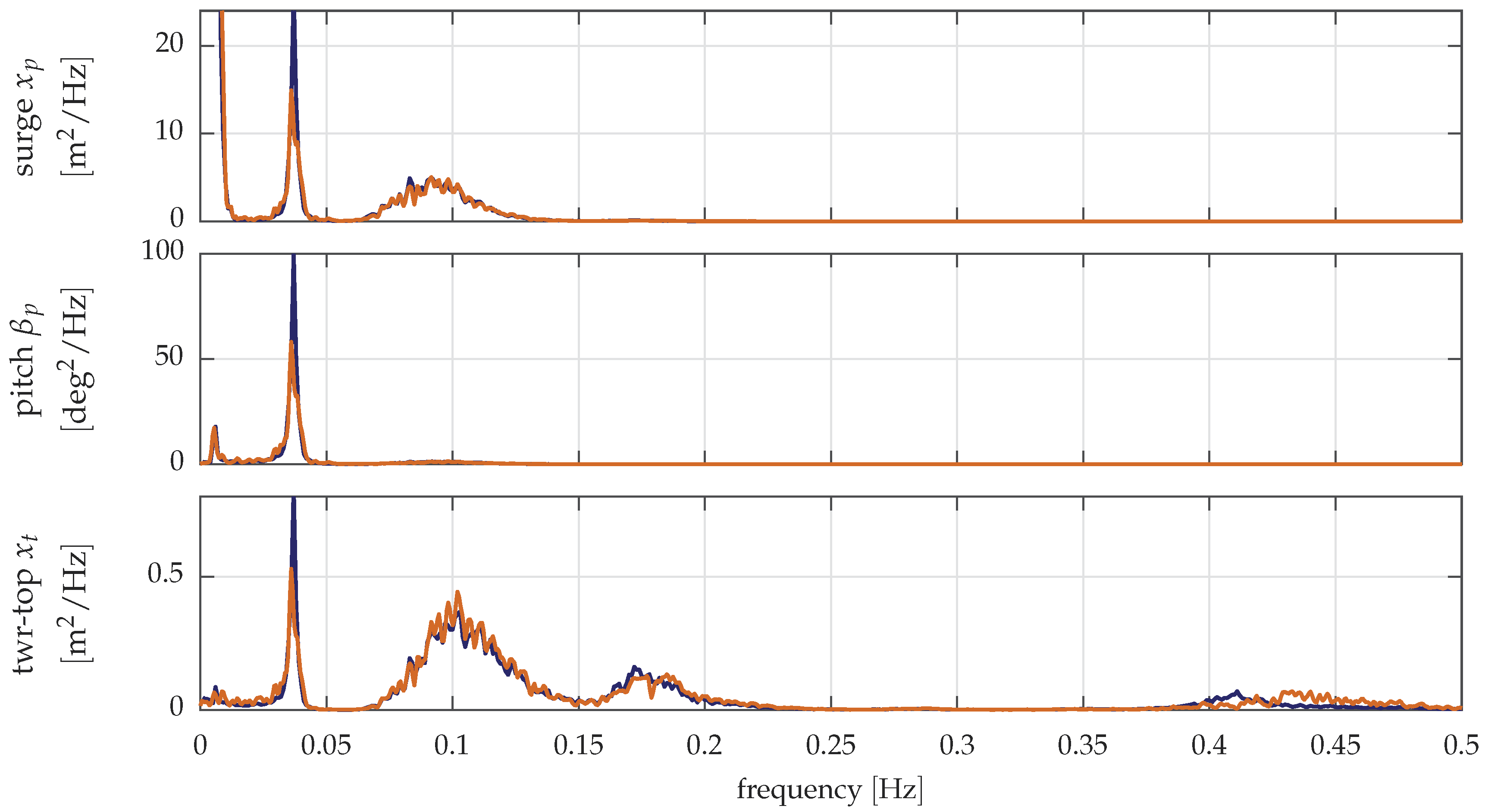
The procedure of Figure 9 will be executed iteratively with $C_{D,hp}=C_{D,hp}\left(\mathit{KC}\right)$. In order to obtain the velocity amplitude $\widehat{v}$ for the estimation of $\mathit{KC}$, the STD of the stochastic response was used with a constant amplification factor. Assuming a Rayleigh distribution of the maximum amplitudes of the nodal velocity response over the columns, it is possible to approximate a representative velocity amplitude $\widehat{v}$. This requires a stationary Gaussian distribution of the platform velocity response, which is a good assumption for wave-induced motions [51]. Here, the mean of the third highest response amplitudes is taken as a reference, the same as for the calculation of the significant wave height $H_s$. The characteristic velocity $\widehat{v}$ is then

$$\widehat{v}\approx k_{peak}\sigma \left(v\right),\mathrm{with}{k}_{peak}=2.0.$$

(15)

The iteration was performed with the simulation model of Section 2.4. The computation was done for a representative load case at above rated winds of Table 2 with the full-scale TripleSpar concept. The resulting generalized damping matrix D over the wind speed bins is shown in Figure 10. A clear dependence of the linearized damping on the environmental bins is observable. It is noted that the wind speeds are correlated with higher sea-states.

One effect driving the observed characteristic is that the linearized drag ${\overline{C}}_{D,ik}^{b\ast }$ increases for larger velocity response amplitudes as shown in Figure 5. The other effect is the KC-dependence for heave plates: Figure 8 shows that the drag coefficient decreases for larger KC-numbers, or larger sea states (given the same periods are present). Thus, two opposing effects drive the sensitivity of ${\overline{C}}_{D,hp}^{b\ast }$ with respect to the velocity amplitude.

The main conclusion drawn from Figure 10 is that the overall generalized damping depends significantly on the sea state, or the load case. This means that neglecting the load case-dependence of the damping might yield an over-conservative estimation of the stability for larger sea-states and likely a too optimistic stability at small sea-states.

Figure 11 shows KC as well as the heave plate drag over all operational wind speeds. Both drag coefficients are shown, the one of the damping problem (blue) and the one of the excitation problem (orange). It can be seen that their qualitative shape is equal, although differences occur for the higher sea-states (see Table 2). The origin of the peak at $\overline{v}=22$ m/s was analyzed. It is not caused by the interaction with the controller. Therefore, it is a result of the system property sensitivities with respect to the operating point and the wind and wave conditions of Table 2. The drag coefficient for the heave plates $C_{D,hp}$ varies in the shown load conditions significantly in the range $C_{D,hp}=11\dots 18$. In the Offshore Code Comparison Collaboration, Continued (OC4) code comparison project [23], a value of $C_{D,hp}=9.6$ was used for all simulations.

3.4. Verification

With the developed iterative procedure, based on the linear frequency-domain SLOW model, the nonlinear drag coefficients of Figure 11 are available as a function of the environmental conditions. These values for $C_{D,hp}$ have been used for the nonlinear FOWT design tool FAST, version 8.16, with all 25 DOFs (including collective blade pitch actuator) enabled. Figure 12 shows the results for an operational case above rated wind. In spite of the reduced number of DOFs of the SLOW model, the main response in surge $x_p$, pitch ${\beta }_p$ and tower-top bending $x_t$ is well reproduced. This holds for the low-frequency response, but also for the first-order wave response. The results show that the low-order model is capable of predicting viable values for the nonlinear heave plate drag $C_{D,hp}$ as a function of the KC-number of the body-response. Nonlinear effects are small enough for a good representation through a frequency-domain model. This does not hold for the nonlinear switching of the wind turbine controller around rated winds and also for the rotor azimuth-dependent blade excitation from wind speeds. The latter effect can be seen in the tower bending $x_t$ at a frequency around $0.43$ Hz.

4. Conclusions

A new method has been developed to iterate the heave plate drag of a FOWT, parameterized as a function of KC, using a low-order aero-hydro-servo-elastic frequency-domain simulation model. The heave plate drag is thus calculated taking into account the FOWT coupled response including the wind turbine controller and excitations from wind and waves. The KC-number is calculated based on this coupled response for each heave plate node.

The procedure involves an efficient representation of the relative fluid between water particles and the body. A separation was made between the drag, responsible for damping and the one responsible for excitation. Despite these simplifications, the comparison of the time series of the drag force has shown a reasonable agreement between the nonlinear and the linearized model.

The employed frequency-domain simulation model is capable of representing the platform motion response, compared to the state-of-the-art engineering model FAST. Thus, the computationally expensive multidisciplinary FOWT system can be reduced to allow for an iterative solution of the viscous drag.

The results show that the heave plate drag varies strongly over realistic operational conditions. A constant drag, which is the common practice for load case simulations, can therefore severely over or underpredict the damping. This is especially important for the fore-aft direction, as the interaction with the wind turbine controller can even further reduce the global damping in this direction. Thus, the proposed method is a realistic means to obtain individual heave plate drag coefficients for each load condition. These coefficients can then be used in higher-fidelity models for a more realistic prediction of the extreme and fatigue loads of FOWTs. A significant advantage of the presented approach is that it is computationally efficient and therefore suitable for concept-level simulations. At this stage, experimental tests or expensive CFD-calculations to obtain the drag coefficients are not yet available.

This study is expected to set off a discussion on how to model the excitation drag, the viscous drag at low-frequencies and possibly the wave drift damping for FOWTs in higher-fidelity models realistically but also approximately in simplified models.

References

1. Tande, J.O.G.; Merz, K.; Paulsen, U.S.; Svendsen, H.G. Floating offshore turbines. Wiley Interdiscip. Rev. Energy Environ. 2015, 4, 213–228. [Google Scholar] [CrossRef]
2. Larsen, T.J.; Hanson, T.D. A method to avoid negative damped low frequent tower vibrations for a floating, pitch controlled wind turbine. J. Phys. Conf. Ser. 2007, 75. [Google Scholar] [CrossRef]
3. Veen, G.V.D.; Couchman, Y.; Bowyer, R. Control of floating wind turbines. In Proceedings of the American Control Conference, Montréal, QC, Canada, 27–29 June 2012; pp. 3148–3153. [Google Scholar] [CrossRef]
4. Lemmer, F.; Schlipf, D.; Cheng, P.W. Control design methods for floating wind turbines for optimal disturbance rejection. J. Phys. Conf. Ser. 2016, 753. [Google Scholar] [CrossRef]
5. Yu, W.; Lemmer, F.; Bredmose, H.; Borg, M.; Pegalajar-Jurado, A.; Mikkelsen, R.F.; Stoklund Larsen, T.; Fjelstrup, T.; Lomholt, A.; Boehm, L.; et al. The TripleSpar Campaign: Implementation and test of a blade pitch controller on a scaled floating wind turbine model. Energy Procedia 2017, 137, 323–338. [Google Scholar] [CrossRef]
6. Jonkman, J. Dynamics Modeling and Loads Analysis of an Offshore Floating Wind Turbine. Ph.D. Thesis, University of Colorado, Boulder, CO, USA, 2007. [Google Scholar] [Green Version]
7. Vaal, J.B.D.; Hansen, M.O.L.; Moan, T. Effect of wind turbine surge motion on rotor thrust. Wind Energy 2014, 17, 105–121. [Google Scholar] [CrossRef]
8. Manolas, D. Hydro-Aero-Elastic Analysis of Offshore Wind Turbines. Ph.D. Thesis, National Technical University of Athens, Athens, Greece, 2015. [Google Scholar]
9. Sant, T.; Bonnici, D.; Farrugia, R.; Micallef, D. Measurements and modelling of the power performance of a model floating wind turbine under controlled conditions. Wind Energy 2015, 18, 811–834. [Google Scholar] [CrossRef]
10. Bayati, I.; Belloli, M.; Bernini, L.; Zasso, A. A formulation for the unsteady aerodynamics of floating wind turbines, with focus on the global system dynamics. In Proceedings of the ASME 36th International Conference on Ocean, Offshore and Arctic Engineering, Trondheim, Norway, 25–30 June 2017. [Google Scholar] [CrossRef]
11. Leble, V.; Barakos, G. Demonstration of a coupled floating offshore wind turbine analysis with high-fidelity methods. J. Fluids Struct. 2016, 62, 272–293. [Google Scholar] [CrossRef] [Green Version]
12. Matha, D. Impact of Aerodynamics and Mooring System on Dynamic Response Of Floating Wind Turbines. Ph.D. Thesis, University of Stuttgart, Stuttgart, Germany, 2016. [Google Scholar]
13. Lin, L.; Vassalos, D.; Dai, S. CFD simulation of aerodynamic performance of floating offshore wind turbine compared with BEM method. In Proceedings of the 26th International Ocean and Polar Engineering Conference, Rhodes, Greece, 26 June–2 July 2016; International Society of Offshore and Polar Engineers: Mountain View, CA, USA, 2016; pp. 568–575. [Google Scholar]
14. Farrugia, R.; Sant, T.; Micallef, D. A study on the aerodynamics of a floating wind turbine rotor. Renew. Energy 2016, 86, 770–784. [Google Scholar] [CrossRef]
15. Tran, T.T.; Kim, D.H. A CFD study of coupled aerodynamic-hydrodynamic loads on a semisubmersible floating offshore wind turbine. Wind Energy 2017, 21, 70–85. [Google Scholar] [CrossRef] [Green Version]
16. Wen, B.; Tian, X.; Dong, X.; Peng, Z.; Zhang, W. On the power coefficient overshoot of an offshore floating wind turbine in surge oscillations (early view). Wind Energy 2018. [Google Scholar] [CrossRef]
17. Liu, Y.; Xiao, Q.; Incecik, A.; Peyrard, C. Aeroelastic analysis of a floating offshore wind turbine in platform-induced surge motion using a fully coupled CFD-MBD method. Wind Energy 2018, 7, 1–20. [Google Scholar] [CrossRef]
18. Journée, J.; Massie, W.W. Offshore Hydromechanics, 1st ed.; Delft University of Technology: Delft, The Netherlands, 2001. [Google Scholar]
19. Fossen, T. Handbook of Marine Craft Hydrodynamics and Motion Control, 1st ed.; John Wiley and Sons: New York, NY, USA, 2011. [Google Scholar]
20. Cummins, W. The impulse response function and ship motion. In Proceedings of the Symposium on Ship Theory, Hamburg, Germany, 25–27 January 1962. [Google Scholar]
21. Morison, J.R. The Force Distribution Exerted by Surface Waves on Piles; Technical Report; University of California, Institute of Engineering Research: Berkeley, CA, USA, 1953. [Google Scholar]
22. Robertson, A.; Wendt, F.; Jonkman, J.M.; Popko, W.; Dagher, H.J.; Gueydon, S.; Qvist, J.; Vittori, F.; Azcona, J.; Uzunoglu, E.; et al. OC5 project phase II: Validation of global loads of the DeepCwind floating semisubmersible wind turbine. Energy Procedia 2017, 137, 38–57. [Google Scholar] [CrossRef]
23. Robertson, A.; Jonkman, J.; Masciola, M.; Song, H.; Goupee, A.; Coulling, A.; Luan, C. Definition of the Semisubmersible Floating System for Phase II of OC4; Technical Report; National Renewable Energy Laboratory: Boulder, CO, USA, 2014.
24. Philippe, M.; Courbois, A.; Babarit, A.; Ferrant, P.; Bonnefoy, F.; Rousset, J.M. Comparison of simulation and tank test results of a semi-submersible floating wind turbine under wind and wave loads. In Proceedings of the ASME 32nd International Conference on Ocean, Offshore and Arctic Engineering, Nantes, France, 9–14 June 2013; ASME: Nantes, France, 2013. [Google Scholar] [CrossRef]
25. Berthelsen, P.A.; Bachynski, E.; Karimirad, M.; Thys, M. Real-time hybrid model tests of a braceless semi-submersible wind turbine. part III: Calibration of a numerical model. In Proceedings of the ASME 35th International Conference on Ocean, Offshore and Arctic Engineering, Busan, Korea, 19–24 June 2016; ASME: Busan, Korea, 2016. [Google Scholar] [CrossRef]
26. Karimirad, M.; Bachynski, E.; Berthelsen, P.A.; Ormberg, H. Comparison of real-time hybrid model testing of a braceless semi- submersible wind turbine and numerical simulations. In Proceedings of the ASME 36th International Conference on Ocean, Offshore and Arctic Engineering, Trondheim, Norway, 25–30 June 2017; ASME: Trondheim, Norway, 2017. [Google Scholar] [CrossRef]
27. Benitz, M.; Schmidt, D.P.; Lackner, M.; Stewart, G.; Jonkman, J.; Robertson, A. Validation of hydrodynamic load models using CFD for the OC4-DeepCwind semisubmersible. In Proceedings of the ASME 34th International Conference on Ocean, Offshore and Arctic Engineering, St. John’s, NL, Canada, 31 May–5 June 2015. [Google Scholar] [CrossRef]
28. Lemmer, F.; Yu, W.; Cheng, P.W.; Pegalajar-Jurado, A.; Borg, M.; Mikkelsen, R.; Bredmose, H. The TripleSpar campaign: Validation of a reduced-order simulation model for floating wind turbines. In Proceedings of the ASME 37th International Conference on Ocean, Offshore and Arctic Engineering, Madrid, Spain, 17–22 June 2018; ASME: Madrid, Spain, 2018. [Google Scholar] [CrossRef]
29. Faltinsen, O.M. Sea Loads on Ships and Offshore Structures; Cambridge University Press: Cambridge, UK, 1993. [Google Scholar]
30. DNV-GL. DNVGL-RP-C205: Environmental Conditions and Environmental Loads Recommended Practice; Technical Report; DNV-GL: Høvik, Norway, 2017. [Google Scholar]
31. Sumer, B.M.; Fredsøe, J. Hydrodynamics Around Cylindrical Structures, 1st ed.; World Scientific: Singapore, 1997. [Google Scholar]
32. Tao, L.; Dray, D. Hydrodynamic performance of solid and porous heave plates. Ocean Eng. 2008, 35, 1006–1014. [Google Scholar] [CrossRef]
33. Lemmer, F.; Amann, F.; Raach, S.; Schlipf, D. Definition of the SWE-TripleSpar Floating Platform for the DTU 10MW Reference Wind Turbine; Technical Report; University of Stuttgart: Stuttgart, Germany, 2016. [Google Scholar]
34. Borgman, L.E. The spectral density for ocean wave forces. In Proceedings of the Santa Barbara Coastal Engineering Conference, Santa Barbara, CA, USA, 11 October 1965; pp. 147–182. [Google Scholar]
35. Pegalajar-Jurado, A.; Borg, M.; Bredmose, H. An efficient frequency-domain model for quick load analysis of floating offshore wind turbines (pre-print). Wind Energy Sci. 2018. [Google Scholar] [CrossRef]
36. Langley, R. On the time domain simulation of second order wave forces and induced responses. Appl. Ocean Res. 1986, 8, 134–143. [Google Scholar] [CrossRef]
37. Lupton, R. Frequency-Domain Modelling of Floating Wind Turbines. Ph.D. Thesis, University of Cambridge, Cambridge, UK, 2014. [Google Scholar]
38. NWTC. NWTC Information Portal (FAST V8); NWTC: Boulder, CO, USA, 2016. [Google Scholar]
39. Bredmose, H.; Lemmer, F.; Borg, M.; Pegalajar-Jurado, A.; Mikkelsen, R.F.; Stoklund Larsen, T.; Fjelstrup, T.; Yu, W.; Lomholt, A.K.; Boehm, L.; et al. The TripleSpar campaign: Model tests of a 10 MW floating wind turbine with waves, wind and pitch control. Energy Procedia 2017, 137, 58–76. [Google Scholar] [CrossRef]
40. INNWIND.EU. Available online: http://www.innwind.eu/ (accessed on 18 August 2018).
41. Stuttgarter Lehrstuhl für Windenergie (SWE), Institut für Flugzeugbau, Universität Stuttgart. Available online: http://www.ifb.uni-stuttgart.de/windenergie/downloads (accessed on 18 August 2018).
42. Jonkman, J.; Robertson, A.; Hayman, G. HydroDyn User’s Guide and Theory Manual; Technical Report; National Renewable Energy Laboratory: Boulder, CO, USA, 2014.
43. Wolfram, J. On alternative approaches to linearization and Morison’s equation for wave forces. Proc. R. Soc. A Math. Phys. Eng. Sci. 1999, 455, 2957–2974. [Google Scholar] [CrossRef]
44. Lemmer, F.; Raach, S.; Schlipf, D.; Cheng, P.W. Parametric wave excitation model for floating wind turbines. Energy Procedia 2016, 94, 290–305. [Google Scholar] [CrossRef]
45. Lemmer, F.; Müller, K.; Pegalajar-Jurado, A.; Borg, M.; Bredmose, H. LIFES50+ D4.1: Simple Numerical Models for Upscaled Design; Technical Report; University of Stuttgart: Stuttgart, Germany, 2016. [Google Scholar]
46. Yu, W.; Lemmer, F.; Schlipf, D.; Cheng, P.W.; Visser, B.; Links, H.; Gupta, N.; Dankemann, S.; Couñago, B.; Serna, J. Evaluation of control methods for floating offshore wind turbines. Energy Procedia 2018, in press. [Google Scholar]
47. Schiehlen, W.; Eberhard, P. Applied Dynamics, 1st ed.; Springer International Publishing: New York, NY, USA, 2014. [Google Scholar]
48. Schwertassek, R.; Wallrapp, O.; Shabana, A.A. Flexible multibody simulation and choice of shape functions. Nonlinear Dyn. 1999, 20, 361–380. [Google Scholar] [CrossRef]
49. Taghipour, R.; Pérez, T.; Moan, T. Hybrid frequency-time domain models for dynamic response analysis of marine structures. Ocean Eng. 2008, 35, 685–705. [Google Scholar] [CrossRef]
50. Krieger, A.; Ramachandran, G.K.V.; Vita, L.; Gómez Alonso, P.; Berque, J.; Aguirre-Suso, G. LIFES50+ D7.2 Design Basis; Technical Report; DNV-GL: Høvik, Norway, 2016. [Google Scholar]
51. Naess, A.; Moan, T. Stochastic Dynamics of Marine Structures; Cambridge University Press: Cambridge, UK, 2012. [Google Scholar]
Figure 1. (a) TripleSpar scaled model (1:60), image reproduced from [39] with permission from Elsevier, 2018, and (b) mechanical sketch of low-order simulation model of Section 2.4 with generalized coordinates.
Jmse 06 00118 g001
Figure 2. Discretized platform shape with nodes of horizontal and vertical drag coefficients. In this work, horizontal drag forces are only applied to the column nodes (dark blue) and vertical drag forces are only applied to the heave plate nodes (light orange).
Jmse 06 00118 g002
Figure 3. Morison excitation transfer functions G Fmor of Equation (8) with magnitude (left) and phase (right) for drag-induced component only with C D = 0.6 and C D , h p = 20 for scaled TripleSpar design of [39]. Top: surge (dark blue) and heave (light orange), bottom: pitch.
Jmse 06 00118 g003
Figure 4. Horizontal body velocity Standard Deviation (STD) σ over column length (left) and obtained linearized drag coefficients C ¯ D (right) for two sea states, Load Case (LC) 7 (dark blue) and LC 9 (light orange) as used in the scaled experiment of [39]. The TripleSpar column with heave plate illustrates the vertical axis in body coordinates.
Jmse 06 00118 g004
Figure 5. Nonlinear (light) and linearized (dark) horizontal Morison drag force component F ¯ D , x 1 for two sea states, LC 7 (grey) and LC 9 (orange) of [39] with indication of velocity STD.
Jmse 06 00118 g005
Figure 6. (a) iterative solution of Morison drag coefficient matrix D for all relevant indices i , j for aligned wind and waves (scaled model of [39], LC 7) and (b) obtained generalized damping matrix.
Jmse 06 00118 g006
Figure 7. Overall Morison drag force time series F D b ( t ) , nonlinear (dark blue) and linearized (light orange) for scaled TripleSpar in LC 9 of [39].
Jmse 06 00118 g007
Figure 8. Vertical drag coefficient C d , h p for heave plates of different porosities (only 0-porosity relevant) with vertical lines for Keulegan–Carpenter (KC) values corresponding to LC 7 (blue) and LC 9 (red) of [39]. Adapted from ([32], p. 1012) with permission from Elsevier, 2018.
Jmse 06 00118 g008
Figure 9. Overview on calculation scheme for Morison drag excitation as well as damping forces as input to linear frequency-domain model. The left column shows the excitation problem, the right column shows the damping problem. The presented approach has distinct procedures for the wave kinematics and the body kinematics. Parametric drag is considered for heave plates.
Jmse 06 00118 g009
Figure 10. Global linearized Morison drag matrix elements for full-scale TripleSpar over environmental conditions of Table 2.
Jmse 06 00118 g010
Figure 11. Heave plate K C -number and resulting quadratic drag coefficient C D , h p from data of Figure 8 for environmental conditions of Table 2. Case (1): Damping (blue) with Closed Loop (CL) system model iterated until convergence. Case (2): Excitation (orange) with body velocity calculated based on panel code RAO and wave kinematics with linear wave theory.
Jmse 06 00118 g011
Figure 12. Model verification: Power Spectral Density (PSD) of response to LIFES50+ operational LC of Table 2 at wind speed v = 17.9   m / s ( H s = 4.3   m , T p = 10   s ). Linearized SLOW model (dark blue), FAST (light orange).
Jmse 06 00118 g012