1. Introduction
Tsunami is a very common hazard that often devastates coastal areas. The prediction of tsunami arrival time is crucial for the effective and wise decisions by tsunami warning centers. As a result, numerical studies have been extensively carried out to simulate tsunami propagation more effectively and efficiently. Traditionally, models utilizing NLSWEs have been used to simulate tsunami generation and to predict tsunami propagation and runup. Notwithstanding the great advantage of very low computational costs, NLSWEs based models do not consider physical dispersion. Alternatively, the utilization of dispersive models using the Boussinesq approach is rapidly growing in tsunami modeling. Dispersive models are also used for the calculation of tsunami propagation in the near shore regions. Nevertheless, this type of models are less computationally efficient as compared to NLSWEs based approaches.
The coastal modeling community has put a lot of attention on modeling wave propagation using BTEs models and, accordingly, many improvements have been reported for the tsunami generation, propagation and runup modeling. Three major advantages of using BTEs over NLSWEs are: the horizontal particle velocity and acceleration over the depth are considered to be varying and the vertical acceleration is not neglected; better prediction of wave propagation over complex topographies can be achieved; and better frequency dispersion effects can be obtained [
1]. Although Navier-Stokes (NS) models are fully dispersive due to the consideration of the complete physics, it is impractical to perform a full solution of the NS equation over large domains, especially for tsunami propagation. Notwithstanding the capability of NS and BTEs models, Horrillo et al. [
2] showed that for practical purposes solutions that are based on the NLSWEs are quite reliable in many circumstances since they give consistent results compared to BTEs and full NS models. More importantly, as discussed, models based on NLSWEs have the great advantage of very low computational costs. Further improvements of NLSWEs models can be achieved by taking the advantage of inherent numerical dispersion errors mimicking physical frequency dispersion of tsunamis. Generally, frequency dispersion consideration is very important to get a precise and realistic prediction of tsunami propagation. In fact, many factors such as refraction, diffraction, nonlinear shoaling, wave-wave interaction, breaking and runup heavily depend on dispersion effects and should be considered to obtain an accurate prediction.
Linear shallow water equations considering numerical dispersion were solved by Imamura et al. [
3] for principal horizontal axes. Cho [
4] improved the algorithm to include the effects of frequency dispersion for diagonal propagation. They both used an algorithm through the modified leap-frog finite difference scheme for discretizing linear shallow water equations to account for the effect of frequency dispersion. This helped to control the inherent numerical dispersion errors of the scheme to cover the effects of physical frequency dispersion for the propagation of tsunami in bathymetries with constant water depth. Later, the approach was extended by Yoon [
5] to a slowly varying bathymetry. He proposed a hidden grid system in which the local water depth determines the grid size for the capturing of dispersion effects. Subsequently, Yoon et al. [
6] developed another scheme using an explicit finite difference method to solve the linearized BTEs and to improve the physical frequency dispersion effects. The linearized BTEs model considers the frequency dispersion effects from shallow to intermediate water regimes accurately [
7,
8,
9,
10,
11,
12,
13,
14]. However, it needs finer spatial and temporal resolutions since the higher order of the derivatives associated with the consideration of the frequency dispersion requires more computational efforts, which is sometimes unnecessary. Establishing an appropriate grid size in NLSWEs models in which the numerical error matches physical frequency dispersion may lead to similar results to BTEs based models with less expensive computational costs.
One of the most commonly used tsunami numerical models is Tohoku University’s Numerical Analysis Model for Investigation of Near-field tsunamis, No. 2 (TUNAMI-N2) [
15] which solves NLSWEs using the finite difference method. This model uses the explicit leap-frog scheme and has been modified to account for frequency dispersion [
3]. The dispersion effects are captured by choosing an appropriate time step and a grid size given by [
3]:
where
is the grid size,
h denotes water depth,
g symbolizes gravity acceleration and
is the time step.
Using a similar approach accounting for the frequency dispersion effects and by using Equation (
1) following the efforts of Imamura et al. [
3] and Cho [
4], a shallow water equations based model named NAMI DANCE was developed [
16]. A brief explanation of NAMI DANCE is presented in the next section. In this study, the ability of NAMI DANCE to capture dispersion effects is examined with several bathymetry profiles or case studies taken from the literature [
5,
6]. The bathymetry profiles are: (i) uniform bottom, (ii) slowly varying depth and (iii) submerged circular shoal. Our objective is to investigate the fact that by selecting an appropriate grid size in NAMI DANCE, we can obtain comparable results to BTEs or NS models in mimicking physical dispersion effects.
3. Gaussian Wave Propagation over Uniform Bottom
The accuracy of the numerical solution of NLSWEs in NAMI DANCE is tested through simulation of a Gaussian hump tsunami as initial free surface [
5,
6] on a constant uniform bottom. In this section, the water surface displacement at certain time steps along horizontal, vertical and diagonal directions are computed and compared with the analytical solution of the linear BTEs [
3,
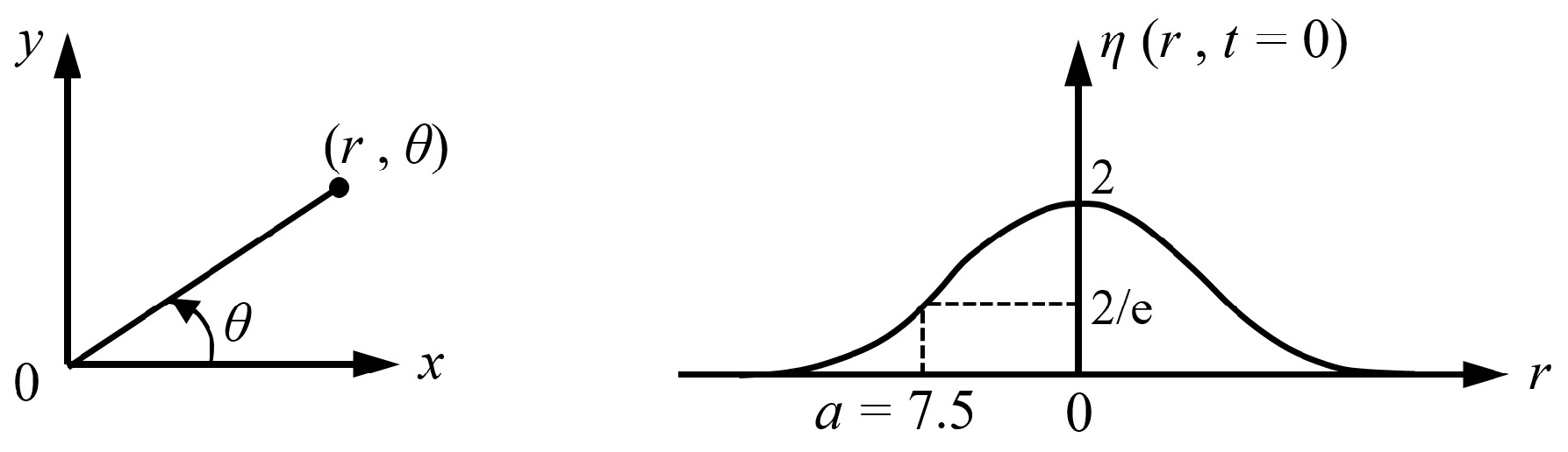
27]. The initial form of the water surface is determined using Gaussian function Equations (
2) and (
3) resulting in the cross sectional shape given in
Figure 1.
In Equation (
2)
a denotes the characteristic radius of Gaussian function,
is the distance of the Gaussian hump from the center,
represents the angle measured counter clockwise from the
x axis,
t represents time and
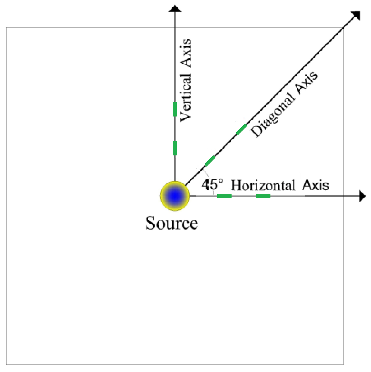
is free surface elevation. Shown in
Figure 2 are the plan view of the initial wave condition, propagation axes, and location of gauges. The analytical solution of the initial Gaussian wave profile was solved by the linear form of the Boussinesq equation given by Carrier [
27] (see
Figure 3):
where
is the zero order Bessel function of the first kind,
k denotes the wave number of uniform waves,
9.81 m/s
,
a is the characteristic radius and
h represents the water depth.
Figure 3 compares snapshots of the water surface profiles at
600 seconds using different numerical methods against the analytical solution of Carrier [
27]. Two different propagation axes (
and
) as well as two different depths (
600 m and
2100 m) are investigated using a uniform bottom domain. The time step is not strongly influenced by a ratio for dispersion and hence, a constant value of
6 s is used following the work of Yoon [
5]. The grid size
is constant according to Equation (
1) and the memory capacity of the hardware/software. In the NAMI DANCE simulations, two different methods are employed to specify the grid size. In the first case, the grid size is selected according to Equation (
1) which provides
1280 m, given
600 m (
Figure 3a,b) and
4287 m for
2100 m (
Figure 3c,d). In the second case, the grid size is selected as
2500 m according to [
5].
Figure 3a,c (
) show that when Equation (
1) is satisfied, NAMI DANCE’s solutions are closer to the analytical results of [
27] and Yoon’s model [
5], while, in diagonal propagation (
Figure 3b,d), Yoon’s [
5] solution leads to more accurate results. Along the diagonal propagation axis (
), more wave dispersion is observed in Imamura et al.’s [
3] results since the dispersion correction term in the diagonal direction is not considered in the solutions, whereas the numerical solution of Yoon is independent of direction [
5]. When Equation (
1) is not satisfied, the numerical solutions of NAMI DANCE do not fit well with the analytical results with the tendency to be closer to Imamura et al.’s [
3] results. It should be mentioned that Yoon’s model considered the dispersion correction term in the diagonal direction [
5]. Yoon’s model is independent of the direction, and therefore its result at
is closer to the analytical solution as compared to those of Imamura’s [
3].
Figure 3c,d show that when Equation (
1) is satisfied (for
4287 m) both Yoon’s [
5] and NAMI DANCE’s results are closer to the analytical solutions compared to other models with Yoon’s solution [
5] being more accurate in the diagonal propagation. In general, the NAMI DANCE’s results for
m,
1280 m and
2100 m,
4287 m compare well with the analytical solution (see
Figure 3).
Figure 3 also indicates that whenever the Equation (
1) is satisfied, physical dispersion of the analytical solution is reproduced with reasonable accuracy by the numerical dispersion of the leap-frog finite difference scheme of NAMI DANCE.
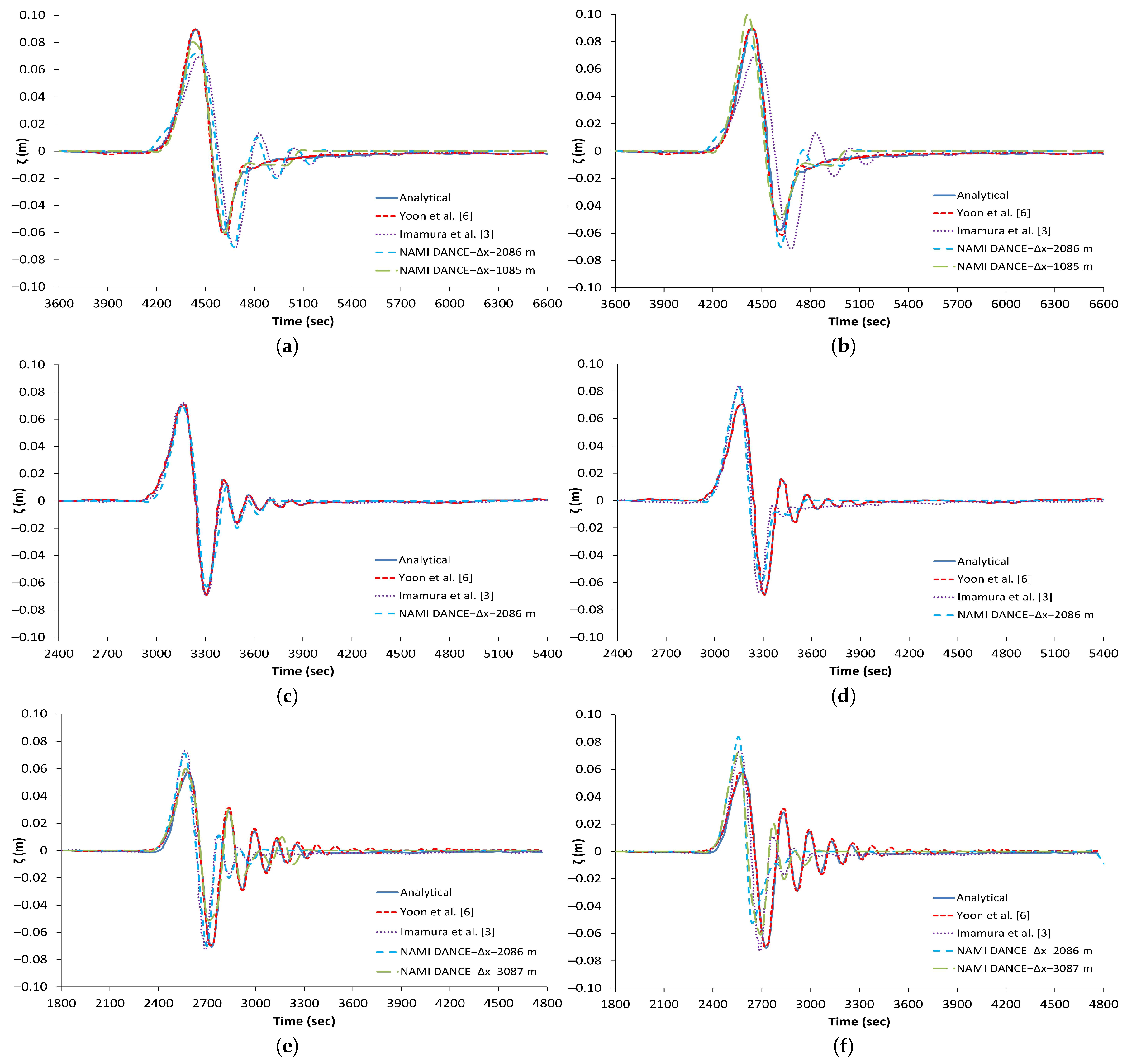
In a separate study, Yoon et al. in 2007 [
6] improved the numerical scheme to reproduce the physical dispersion effects and tested on a uniform bottom domain with different water depths [
6]. Shown in
Figure 4 are the results which compare time histories of the water surface profiles at a distance of 312,900 m (150
and
2086 m) away from the center of the initial Gaussian hump obtained by different models including Yoon et al.’s [
6] model. Here, three different depths and two different propagation axes are investigated (
500 m,
1000 m and
1500 m with
and
). Again, in the simulations with the NAMI DANCE model two different methods are employed to specify the grid size. In the first case, the grid size is selected according to Equation (
1) which provides
1085 m for
500 m (
Figure 4a,b),
2086 m for
1000 m (
Figure 4c,d) and
3087 m for
1500 m (
Figure 4e,f). In the second case, the grid size is selected as
2086 m according to [
6].
Figure 4a,c,e (
) show that when Equation (
1) is satisfied, NAMI DANCE’s results are closer to the analytical solution of Carrier [
27] and Yoon et al.’s [
6] results as compared to other models, while, in diagonal propagation (
Figure 4b,d,f) Yoon et al.’s [
6] solution leads to more accurate results. On the other hand, more dispersion effects are observed in Imamura et al.’s [
3] results, since the dispersion correction term in the diagonal direction is not considered in the solutions. When Equation (
1) is not satisfied in NAMI DANCE, the results do not fit well with the analytical solutions having a tendency to be closer to Imamura et al.’s [
3] results. In addition, on the diagonal propagation, NAMI DANCE results show less dispersive behavior as compared to other models. The solutions predicted by Yoon et al.’s [
6] model are closer to the analytical solution than those of Imamura et al.’s [
3] model since the dispersion correction term in the diagonal direction is considered in Yoon et al.’s [
6] model.
In general, NAMI DANCE’s results for
1085 m given
500 m,
2086 m given
1000 m and
3087 m given
1500m, compare well with the analytical solution. However, along the diagonal propagation axis the water surface profiles are slightly higher than the analytical solution. In addition, whenever Equation (
1) is satisfied in NAMI DANCE, physical dispersion of the Boussinesq equations is reproduced with reasonable accuracy by the numerical dispersion of the leap-frog finite difference scheme. It is also worth mentioning that the choice of the space discretization by Equation (
1) can unresolve the wave length, given the insufficient points per wave length to provide the approximation needed for accuracy of numerical solutions, as pointed out in earlier work [
3]. However, this basic low resolution (points per wave length) is needed to create the numerical dispersion required to reproduce the physical dispersion.
4. Gaussian Wave Propagation over Slowly Varying Depth
The above-mentioned wave propagation model (proposed by Yoon [
5]) uses a uniform bottom and therefore is not applicable for a varying bathymetry. Alternatively, Yoon [
5] developed a new finite difference adjustable grid scheme which satisfies the local wave frequency dispersion in both varying and flat bathymetries. He showed that this new scheme provides a noticeable improvement on the effect of frequency dispersion compared to the schemes of Imamura et al. [
3] and Cho [
4].
In this section, the one-dimensional water surface displacement at certain time along the horizontal direction is computed with NAMI DANCE and compared with the solutions of Yoon’s [
5] model, adjustable grid model [
5] and Imamura et al.’s [
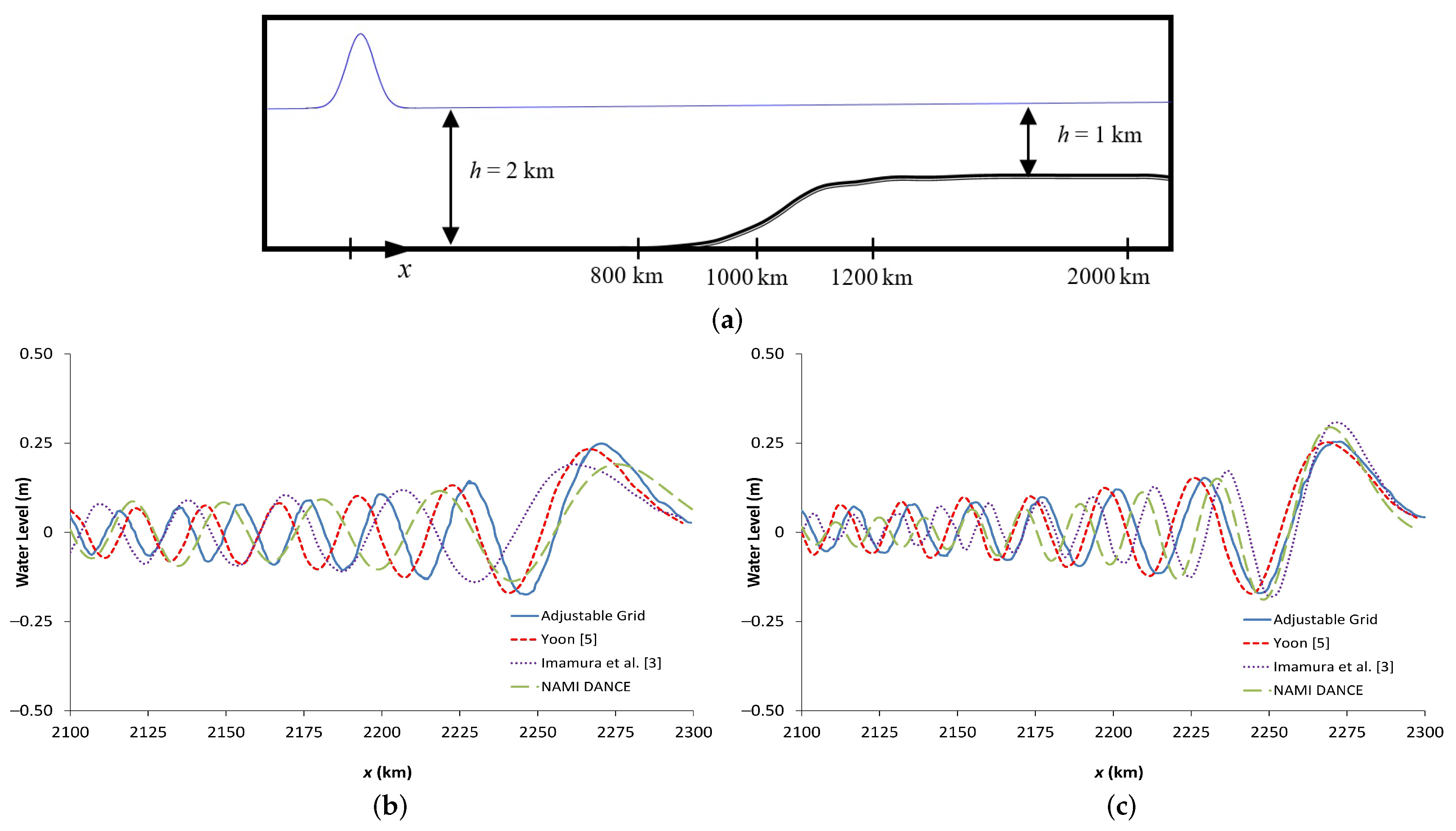
3] model. The wave propagation is over a slowly varying bathymetry consisting of two uniform water depths,
2 km and 1 km, connected by a half-sine function (
Figure 5a). The initial water surface profile is determined using the same Gaussian profile defined by Equations (
2) and (
3) (
Section 3).
Figure 5b,c compare snapshots of the water surface profiles at time 40,000 s using different numerical methods indicated above against the numerical solution of Yoon’s (2002) adjustable grid. In the simulations, NAMI DANCE employed two different grid sizes selected according to the Equation (
1) which provides
4 km, given
2 km (
Figure 5b) and
2 km for
1 km (
Figure 5c). Simulations were done using a uniform grid size for the entire domain, even though a slowly varying bottom with two different depths were considered.
In general, results show that when Equation (
1) is satisfied, NAMI DANCE’s solutions are closer to both Yoon’s [
5] models. However, when a low resolution grid size (4 km) was used in NAMI DANCE, a smaller dispersive effect was observed in the tail of the wave train. Since the large grid size leads to having a smaller numerical dispersion than physical dispersion, smaller tailing waves are created.
5. Solitary Wave Propagation over a Submerged Circular Shoal
Using a finite difference model, Yoon et al. [
6] developed a dispersion-correction parameter to solve Boussinesq type wave equations which could be applied to more general varying bathymetries, e.g., two dimensions. In the model proposed by Yoon et al. [
6], the numerical dispersion effect is determined by the local water depth variations and time step, presenting good performance especially for cases featuring short waves. Yoon et al. [
6] presented the evolution of a tsunami wave over a submerged circular shoal and since there is no analytical solution available for this case, they compared their solutions with those of the linearized Nwogu’s Boussinesq equations [
7] implemented in the FUNWAVE code [
8,
9].
FUNWAVE is a fully nonlinear Boussinesq wave model and has been improved for the dispersion relationship of short waves. In BTEs based models, the grid size should be small enough to avoid the dependency of numerical dispersion effects on higher order terms. Therefore, FUNWAVE’s results with smaller grid size are more reliable.
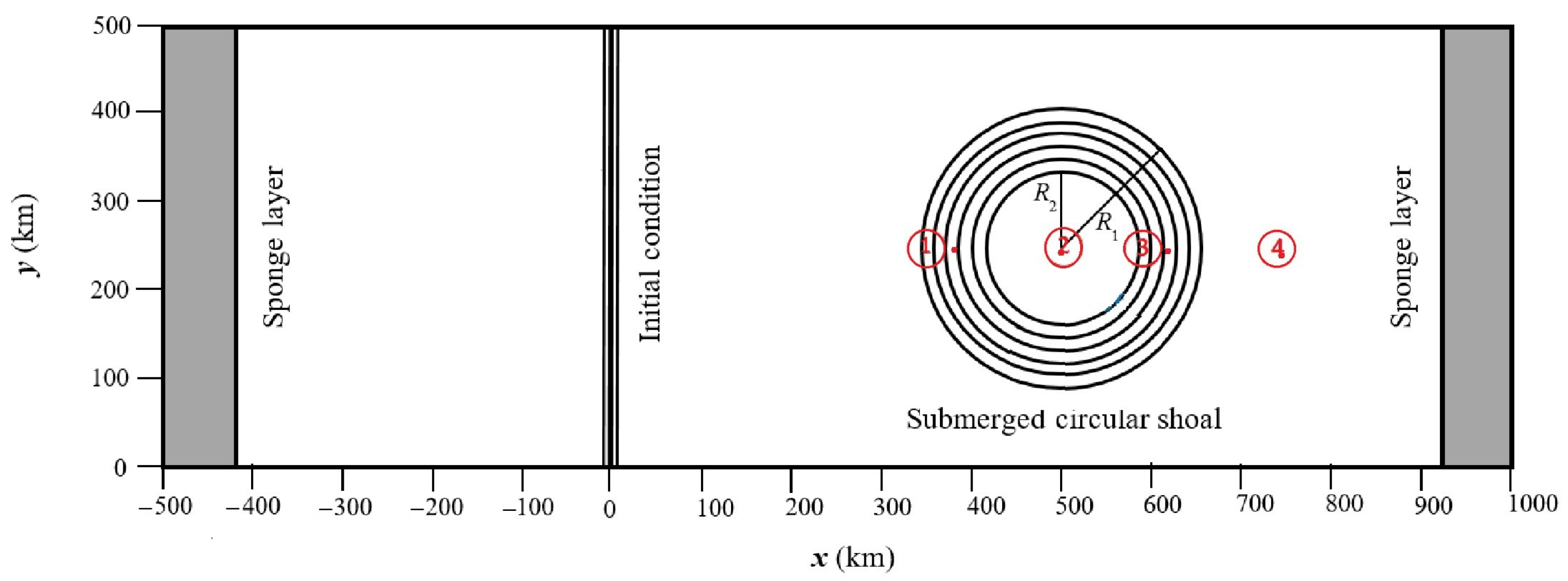
Figure 6 shows the domain configuration with size of 1500 km × 500 km. The center of the submerged circular shoal is located at
500 km,
250 km. The water depth of the numerical domain over the shoal is given by:
where
is the distance from the center of the submerged circular shoal,
km is the base radius and
km is the top radius.
The initial form of the water surface is given in the form of a soliton as:
The gauges 1 and 3 are located on the slope of the circular shoal with depth of 1000 m. Gauge 2 is placed at the center of the circular shoal with 500 m water depth and Gauge 4 is at
750 km, see
Figure 6. In order to dissipate the outgoing wave energy, Yoon et al. [
6] considered sponge layers at the two ends of the numerical domain. The grid size was selected as
2000 m and the time step
4 s. The water surface displacements at these numerical gauges were also computed with NAMI DANCE and compared with the FUNWAVE’s results to test our model capability to reproduce the physical dispersion effects. Simulations with FUNWAVE were conducted with two different grid sizes (
500 m and
2000 m). The grid size in NAMI DANCE is selected as 3000 m to satisfy Equation (
1).
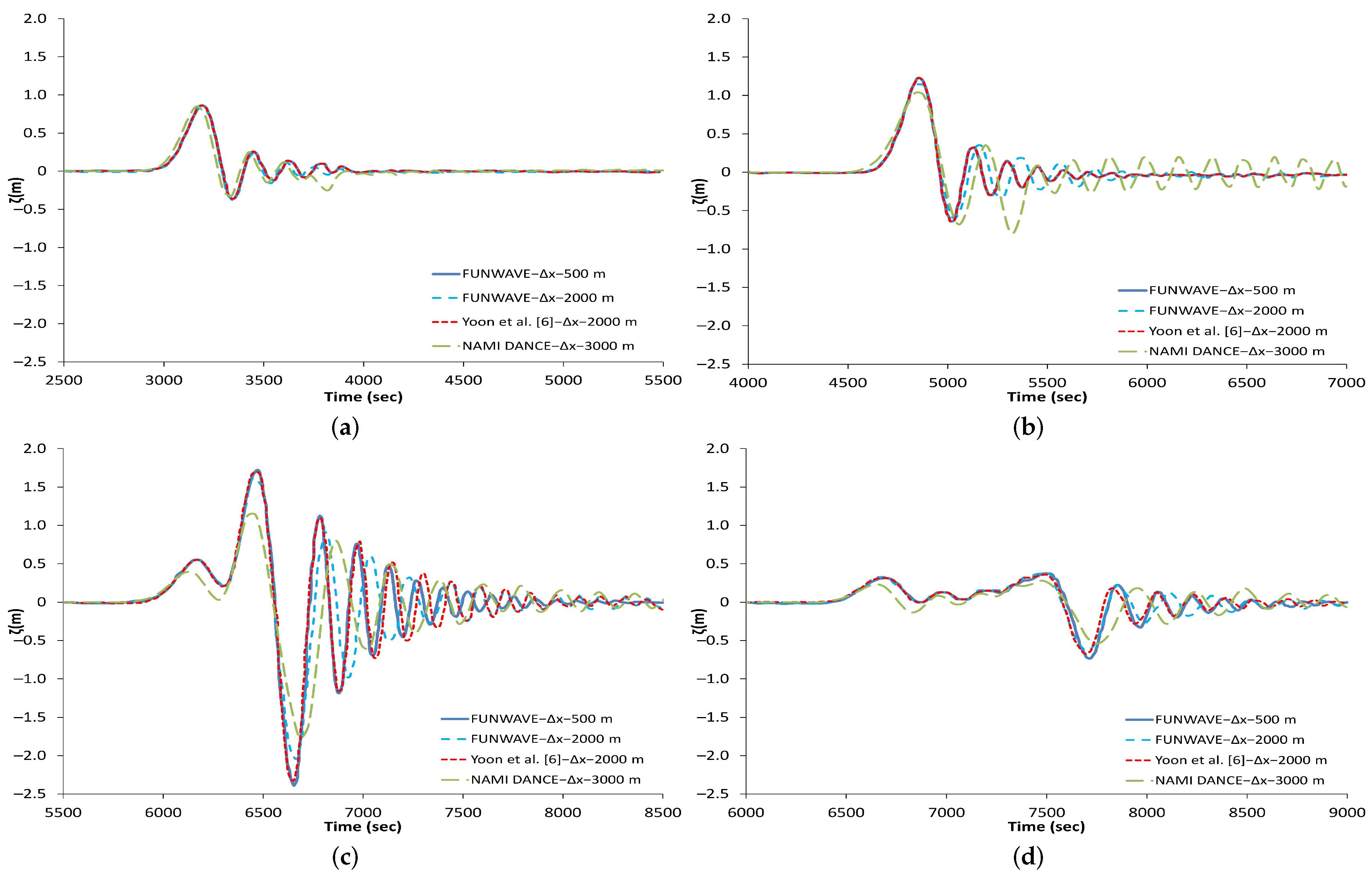
Figure 7 compares time series of the water surface profiles at different numerical gauges. The simulations are carried out for 9000 seconds from the initial soliton wave condition. In general, the first wave matches well with the FUNWAVE’s results but later NAMI DANCE’s results show less dispersive behavior compared to both, Yoon et al. [
6] and FUNWAVE [
6].
Figure 7a shows the time history of water surface profiles recorded at numerical gauge 1 (1000 m water depth). It is clearly seen that NAMI DANCE matches very well with the other results, especially with FUNWAVE (
2000 m), although, some small discrepancies are seen in the tail of the time series. This good match is attributed to the model capability to mimic the physical dispersion and also to the minor effects caused by refraction and shoaling.
Figure 7b shows the time history of water surface profiles computed at numerical gauge 2 which is located at the center of the circular shoal at a water depth of 500 m. In general, NAMI DANCE’s first two wave results are in good agreement with both, FUNWAVE and Yoon et al.’s [
6] results. The first wave is slightly under predicted, as a consequence, a small phase lag is observed in the following wave. When the first wave is smaller than predicted, tail waves occur in order to satisfy the energy conservation.
The time history of the water surface profile on the back side of the circular shoal (1000 m depth) at numerical gauge 3 is shown in
Figure 7c. At this gauge, NAMI DANCE’s result shows a smaller wave amplitude and a slightly longer period. However, in general, results are considered reasonable if we account the accumulating effect of numerical dispersion through the shoaling process.
Figure 7d confirms the model’s capability to reproduce well the water surface profile at the lee part of the circular shoal (1500 m depth), numerical gauge 4. Although the wave went through a varying bathymetry as well as the shoaling process, the agreement of the NAMI DANCE solution with FUNWAVE result is quite good indicating that the model approach works well in mimicking the physical dispersion proving that a correct grid size and time step are chosen. Thus, the NAMI DANCE model is a good option to be applied in practical tsunami modeling that requires dispersion effects.
It is noticeable that the first waves play the main role in tsunami inundation problems, however, inundation is outside the scope of this study.


