Abstract
The purpose of the paper is to take advantage of recent work on the study of resonantly forced baroclinic waves in the tropical Pacific to significantly reduce systematic and random forecasting errors resulting from the current statistical models intended to predict El Niño. Their major drawback is that sea surface temperature (SST), which is widely used, is very difficult to decipher because of the extreme complexity of exchanges at the ocean-atmosphere interface. In contrast, El Niño-Southern Oscillation (ENSO) forecasting can be performed between 7 and 8 months in advance precisely and very simply from (1) the subsurface water temperature at particular locations and (2) the time lag of the events (their expected date of occurrence compared to a regular 4-year cycle). Discrimination of precursor signals from objective criteria prevents the anticipation of wrong events, as occurred in 2012 and 2014. The amplitude of the events, their date of appearance, as well as their potential impact on the involved regions are estimated. Three types of ENSO events characterize their climate impact according to whether they are (1) unlagged or weakly lagged, (2) strongly lagged, or (3) out of phase with the annual quasi-stationary wave (QSW) (Central Pacific El Niño events). This substantial progress is based on the analysis of baroclinic QSWs in the tropical basin and the resulting genesis of ENSO events. As for cold events, the amplification of La Niña can be seen a few months before the maturation phase of an El Niño event, as occurred in 1998 and 2016.
1. Introduction
Governments, private companies, and individuals are demanding ever-more sophisticated climate services, as manifested by the Global Framework for Climate Services (GFCS). Understanding and forecasting of the onset and duration of the phases of the El Niño-Southern Oscillation (ENSO) has provided a basis for the routine delivery of seasonal climate outlooks and associated information and services for regions impacted by the ENSO (e.g., [1,2]).
The warming phase is known as El Niño and the cooling phase as La Niña. The Southern Oscillation is the accompanying atmospheric component, coupled with the sea temperature change; El Niño is accompanied with high, and La Niña with low air surface pressure in the tropical western Pacific. The current generation of ENSO prediction models forecast ENSO 1 year in advance [3], through oceanic memory associated with subsurface temperature anomalies along the equatorial thermocline [4]. Variations in the thermocline depth along the equator serve as the major source of predictability of sea surface temperatures (SSTs), as evidenced by coherent variations with the observed equatorial warm water volume (WWV) that precedes the ENSO by two to three seasons [5]. Oscillations of the thermocline modulate equatorial SST anomalies through the vertical advection of warm water in the central-eastern equatorial Pacific. In a recent work, the role of surface forcing in the observed variability of subsurface ocean temperatures was discussed, and the components of surface forcing were investigated to determine which plays a more important role [6].
However, the evolution of climate prediction systems has not kept pace with forecasting requirements in terms of accuracy and reliability [7,8,9]. We are at a critical stage in observing and predicting the El Niño-Southern Oscillation (ENSO). This presents an opportunity for scientists, technological experts, engineers, and operational climate services to re-engage and achieve major change [10].
Provided that the amplitude and date of occurrence of the warm ENSO events are properly defined, the paper relies on observations showing that both can be forecasted between 7 and 8 months in advance precisely and very simply, as well as the expected potential climate impact.
2. Recap of Previous Papers about Quasi-Stationary Waves (QSWs) in the Tropical Pacific
The objective of this paper is to show how to reduce the systematic and random prediction errors of the statistical models currently used by taking advantage of the dynamics of resonantly forced baroclinic waves in the tropical Pacific. Indeed, any improvement in forecasting techniques is based on a better understanding of the baroclinic quasi-stationary waves (QSWs) that produce ENSO events.
2.1. Baroclinic QSWs in the Tropical Pacific
The tropical Pacific is influenced by coupled baroclinic QSWs guided by the equator, of different periods. They are resonantly forced, that is, their natural period coincides with the forcing period. The coupling of QSWs occurs if waves share the same modulated currents required to maintain a geostrophic motion.
QSWs are characterized by antinodes at the sea surface height (SSH) anomalies, reflecting the pycnocline depth, and nodes associated with modulated geostrophic currents. Although these terms—node and antinode—are unfair because the observed baroclinic waves are not standing waves, this terminology is convenient for describing QSWs, that is, SSH anomalies that are reproducible from one cycle to another, and the resulting modulated current velocity anomalies supposing a quasi-geostrophic motion.
The wavelet transform has proven to be convenient for the analysis of localized variations of power within a time series. By decomposing a time series in time-frequency space, one is able to determine both the dominant modes of variability and how those modes vary in time. Using a temporal reference (e.g., the Southern Oscillation Index SOI), the cross-wavelet analysis expresses the amplitude of anomalies (regardless of the time when the anomaly reaches its maximum), and the phase (the time evolution, that is, the time when the anomaly reaches its maximum over a given period).
QSWs are highlighted by using the cross-wavelet analysis of the SSH and the surface current velocity (SCV) anomalies to represent the amplitude and phase of the antinodes and nodes [11]. Therefore, three QSWs with average periods of 1, 4, and 8 years cross the tropical Pacific Ocean.
2.1.1. The Annual QSW
The annual QSW is formed by an equatorial first baroclinic, fourth meridional mode Rossby wave resonantly forced by easterlies [11] (Figure 1a,b). During the annual cycle, the quasi-geostrophic equilibrium of the tropical basin results in the modulated components of the North Equatorial Counter-Current and the South Equatorial Current (Figure 1c,d), both forming a single dynamical system as a part of the annual QSW.
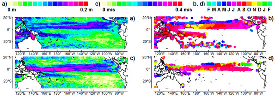
Figure 1.
Amplitude (left) and phase (right) relative to August 1999, averaged in the 8–16 month band of: (a,b) antinodes, (c,d) zonal velocity u (facing east) at the nodes. The choice of colors to represent the phase in (b,d) reflects the periodicity of the observed phenomenon; the amplitude remains nearly the same in February, whatever the year. The sea surface height (SSH) is provided by the French CNES (Centre National d’Etudes Spatiales): www.aviso.oceanobs.com. The geostrophic surface current velocity field (SCV) is obtained through the OSCAR (Ocean Surface Current Analyses: Real time) program and provided by the NOAA (National Oceanic and Atmospheric Administration): www.oscar.noaa.gov/datadisplay/datadownload.htm.
In addition to the two modulated currents at the nodes of the annual QSW, two zonal bands are displayed in the northern hemisphere at the antinodes. By contrast, in the southern hemisphere, the two antinodes which should be symmetrical to the two previous ones are barely visible, except in the western part of the tropical basin.
2.1.2. The Quadrennial QSW
The quadrennial QSW is formed from an equatorial first baroclinic mode Kelvin wave, as well as first baroclinic first meridional mode equatorial and off-equatorial Rossby waves [11]. The equatorial Rossby wave is mainly diverted to the north as an off-equatorial Rossby wave as it approaches Indonesia. This is enabled because the Rossby wave whose westward phase velocity is 0.3 m/s at 8° N is embedded into the North Equatorial Counter-Current (NECC), whose eastward velocity at that time is higher.
Three antinodes are visible in Figure 2a,b, two off-equatorial antinodes in the western Pacific and one equatorial antinode in the central-eastern Pacific. During the quadrennial cycle, the quasi-geostrophic equilibrium in the tropical basin results in the 4-year average period modulated component of the South Equatorial Current (Figure 2c,d).
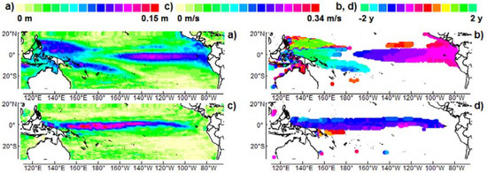
Figure 2.
Amplitude (left) and phase relative to November 1997 (right) averaged in the broadband 1.5–7 years of (a,b) antinodes, (c,d) zonal velocity u (facing east) at the nodes; –SOI (the opposite of SOI) is used as the reference signal so that the phase is expressed relative to the maximum of –SOI, that is, the maturation phase of El Niño in November 1997. The monthly Southern Oscillation Index (SOI) is provided by the National Center for Atmospheric Research: www.cgd.ucar.edu/ cas/catalog/climind/soi.html.
2.1.3. The 8-Year Period QSW
The 8-year period QSW formed by second baroclinic mode Kelvin and Rossby waves appears to be a subharmonic of the quadrennial QSW [11]. Its amplitude is lower than that of the quadrennial QSW and it does not reach the easternmost part of the basin; therefore, its contribution to the genesis of the ENSO is weak.
2.1.4. Genesis of the ENSO
According to the current theory, the ENSO is defined by its effects, that is, an irregularly periodic variation in winds and SST over the tropical eastern Pacific Ocean, affecting much of the tropics and subtropics. As part of this work, the ENSO is defined exclusively by the phases of the quadrennial QSW, which involves a study area of the tropical Pacific included between 20° N and 30° S. ENSO events reach their maturation phase at the end of the eastward phase propagation of the quadrennial QSW that owes its existence to both its coupling with the annual QSW, as well as to the ENSO events themselves [11]. The coupling with the annual QSW occurs as they share the same modulated current at the nodes, from which results a mean flow. As the annual and the quadrennial QSWs behave as coupled oscillators with inertia, a subharmonic mode locking occurs [12]. This means that the mean period of the quadrennial wave is a multiple of the mean period of the annual QSW, that is, 4 years precisely.
Stimulation of the quadrennial QSW from the ENSO results from the evaporation of subsurface warm waters when they are raised to the surface in the central-eastern Pacific, at the end of the eastward phase propagation. The subsequent cooling of the surface water causes the thermocline to rise due to convection processes, which forces the recession of the QSW while initiating its westward phase propagation. In some cases, upwelling in the eastern Pacific is strongly stimulated while the quadrennial QSW recedes to the west. The westward phase propagation of the quadrennial QSW then causes a pumping effect, resulting in the transfer of cold water to the central-western Pacific. The quadrennial QSW is self-sustained, although its period is subject to a large variability, varying between 1.5 and 7 years, in contrast to the annual wave period that is paced by the forcing period enforced by the easterlies.
The quadrennial QSW divides the tropical Pacific into western and eastern antinodes, both of them being in nearly opposite phases. This partition of the tropical Pacific is well known to oceanographers. The western antinodes, which result from off-equatorial Rossby waves, have a warm water storage function. The subsurface water temperature at the central-eastern antinode, which produces the ENSO, reflects the recharge of that antinode. In this respect, it anticipates the maturation phase of the ENSO even earlier as the measurement is performed further west. This can be seen in the amplitude and phase averaged in the broadband 1.5–7 years of SSH anomalies, using –SOI (the opposite of SOI) as the reference signal in the cross-wavelet analysis of SSH so that the phase is expressed relative to the maturation phase of El Niño (Figure 2a,b).
At the longitude of 180° W, that is, at the most westerly tip of the equatorial central-eastern antinode, the subsurface water temperature anomalies precede the maturation phase of the ENSO by 7–8 months. This is close to the limit beyond which it is theoretically impossible to predict the ENSO from direct observations, because the central-eastern antinode vanishes west of 180° W. Also, beyond 7–8 months prior to the ENSO, the ocean cannot deliver a straightforward precursor signal, as the central-eastern antinode has not been formed yet. Any prediction attempt of warm events should then focus on the observation of early phenomena leading to the formation of that antinode, which would necessarily involve interactions between the annual and quadrennial QSWs.
However, along the equator at 180° W, the southernmost antinode in the northern hemisphere of the annual QSW is also perceptible (Figure 1a,b), indicating an overlap of the antinodes of the annual and quadrennial QSWs. Indeed, resonantly forced by easterlies, the annual QSW has a large amplitude in the northern hemisphere, exhibiting two antinodes nearly parallel to the equator, around 8–10° N and 0–4° N. On the other hand, the two antinodes located in the southern hemisphere display a weaker amplitude resulting from weaker trade wind stress, with the exception of their western part.
Since only the quadrennial QSW should be involved in the prediction of the ENSO, the results obtained when the oscillation of the thermocline is observed without discrimination are therefore vitiated by significant systematic and random errors due to the superposition of annual and quadrennial QSWs.
2.2. Defining the ENSO Maturation Phase by the SST Leads to Ambiguous Results
The characterization of warm ENSO events according to the SST, as practiced very widely since the work of Trenberth [13], is extremely complex because of the extreme complexity of exchanges at the ocean-atmosphere interface. For example, convection processes in the central-eastern Pacific heat the surface of the ocean, which stimulates evaporation. Since this produces a cooling of the surface, the SST measurement results from two phenomena whose effects are antagonistic, which makes its value uncertain. In some cases, the sign of SST anomalies may not even be what is expected, as happens for some values of the lag of the quadrennial QSW, that is, the date (month and year) of appearance compared to a regular 4-year cycle [14,15]. This gives each event a unique signature in the SST lifecycle.
It is more appropriate to characterize the ENSO from the fall of the Southern Oscillation Index (SOI), which indicates the maturation phase without any ambiguity. However, the SOI is defined as the pressure difference between Tahiti and Darwin, which are both located well south of the equator and thus away from the main centers of action of El Niño. Since the time lag of El Niño characterizes different modes of variability [14], the question of the atmosphere’s sensitivity to inter-El Niño variations of the SST is not essential. In contrast, the predictability of the impact of the ENSO locally (e.g., [16]) closely depends on the lag of the event.
3. Method
The improvement of the ENSO forecast is based (1) on integrating the subsurface water temperature at a place representative of the quadrennial QSW (the QSW responsible for the ENSO) and (2) on omitting the SST, whose anomalies measured in the central-eastern Pacific are of no use, neither to characterize the different modes of variability of the ENSO nor to quantify heat fluxes. Indeed, SST anomalies result from a balance at the ocean-atmosphere interface and are hardly involved directly in the fluctuations of the latent heat flux, which is essentially governed by convection processes in both the upper ocean and the low-level atmosphere at the basin scale.
Regarding the climate impact of the ENSO, the time lag of the events characterizes their modes of variability instead of the SST, which is usually employed (Figure 3). Thus, the dominant mode of variability of the ENSO can be expected 7–8 months in advance, when the date of occurrence can be estimated. Indeed, according to the time lag, the quadrennial QSW—whose natural period is 4 years—benefits more or less optimally from the geostrophic forces in the tropical basin. On the other hand, the time lag defines the mode of coupling between the annual and quadrennial QSWs.
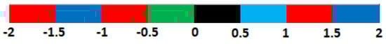
Figure 3.
The time lags (in years) within the four-year cycle. In red, the El Niño-Southern Oscillation (ENSO) event is out of phase with the annual quasi-stationary wave (QSW); in green it is unlagged; in light blue it is weakly lagged; and in dark blue it is strongly lagged. Black represents the forbidden lag (no event can occur).
Let us recall what the modes of variability associated with the lag are, as well as their frequency of occurrence [11,15]. First, there is a need to distinguish events out of phase with the annual QSW (red regions), whose probability of occurrence is f = 19%, from those in phase with the annual QSW (the remaining part, that is, f = 81%). Events in phase with the annual QSW induce heat transfer in the central Pacific (CP), while the transfer occurs in the eastern Pacific (EP) in the other cases.
The events in phase are divided into three classes according to whether they are unlagged (green region, f = 31%), weakly lagged (light blue region, f = 18%), or strongly lagged (dark blue regions, f = 32%). They always occur during the second semester of the year (nearly a third of them are unlagged). The impact on the SOI is even lower when the event is more lagged. However, concerning heat transfer that occurs in the eastern Pacific (EP), whatever the lag, the climate impact of such events has many similarities. Highlighting the small discrepancies, if they exist, would require a statistical analysis of a number of events, requiring more data than is currently available. We will therefore have to limit our deductions to a few hypotheses.
The forbidden lag (black region) shows that no unlagged event can be out of phase with the annual QSW. This information is important for the anticipation of events, which cannot occur during the first semester every four years. Statistical analysis referring to ENSO events that have occurred for more than a century reveals other useful information on the probability of occurrence of events out of phase (CP). It is f = 14% for −2 years < lag < −1.5 years, f = 43% for −1 year < lag < −0.5 years, and f = 43% for 1 year < lag < 1.5 years. This means that almost all CP events occur either when −1 year < lag < −0.5 years or 1 year < lag < 1.5 years, that is to say, exclusively during the first semester every two years: no EP event can occur at the same time.
4. Results
4.1. Cold Events
Upwelling in the eastern Pacific may be strongly stimulated during the westward phase propagation of the quadrennial QSW. In this case, the cold water that extends on the surface generates nonlinear processes leading to the amplification of easterlies during La Niña recovery. Such amplification effects occurred twice during the observation period so that their triggering is quite common (Figure 4). From the measurement of subsurface water temperature in the central Pacific, their forecast is carried out a few months before the maturation phase of the ENSO event, as a result of the transfer of cold water to the central-western Pacific during the westward phase propagation of the quadrennial QSW.
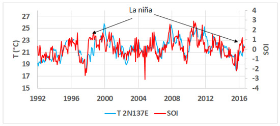
Figure 4.
Comparison of the mean subsurface water temperature measured between 100 and 200 m in depth at 2° N 137° E (TAO; Tropical Atmosphere Ocean Project http://www.pmel.noaa.gov/tao/) to the Southern Oscillation Index (SOI) (https://www.ncdc.noaa.gov/teleconnections/enso/indicators/soi/). Modern means of investigation show that the correlation between the subsurface water temperature and the ENSO amplitude is even closer than Vilhelm Bjerknes had imagined.
4.2. A Linear Relationship between the SOI and Subsurface Water Temperature at 2° S 180° W
A relationship between the SOI and heat content in subsurface water in the western Pacific has been known for some time (e.g., [17,18,19]), and this is evident in Figure 4 where the mean subsurface water temperature measured between 100 and 200 m in depth at 2° N 137° E is compared to the SOI.
As previously mentioned, the tropical Pacific is subject to three QSWs whose mean periods are 1, 4, and 8 years. The resulting oscillation of the pycnocline depth reflects the superposition of the different baroclinic waves along the equator. Taking advantage of the weakness of the amplitude of the two zonal antinodes of the annual QSW in the central-eastern part of the southern hemisphere, the peaks of the subsurface water temperature at 2° S 180° W show that the contribution of the quadrennial QSW is enhanced, to the detriment of the annual QSW. Indeed, the central-eastern antinode of the quadrennial QSW, that is, the QSW that generates the ENSO, is symmetrical with respect to the equator. In particular, at 2° S its amplitude is as strong as it is on the equator at the same longitude. In such conditions, the peaks either reflect the annual QSW or the quadrennial QSW distinctly, without any interference. What is true for the central-eastern antinode of the quadrennial QSW is also true for the 8-year period QSW that contributes less to the ENSO.
Excluding the two periods marked by the resumption of La Niña following the mature El Niño events in November 1997 and September 2015, during which nonlinear processes occurred, the SOI’s signature is reflected faithfully and in detail by the subsurface water temperature in the westernmost part of the equatorial Pacific. This confirms and clarifies the observations made before the Tropical Atmosphere Ocean Project (TAO) became operational.
Seven ENSO events are observable from the beginning of the TAO project, that is, spanning from late 1992 to 2017. The correlation between the minimum SOI and the monthly subsurface water temperature at 2° S 180° W averaged 125 to 175 m in depth (data are interpolated between 150 and 200 m), 7–8 months prior to the minimum SOI (Table 1, Figure 5a), indicating that the coefficient of determination is 0.96. This reflects both the strong coherency between that temperature T and the minimum SOI, and the accuracy of measurements when the SOI is filtered within the band of 1.5/15 years. To show the merits of the method, filtering the SOI signal is essential to reduce the noise in order to highlight the amplitude and the location of the successive minima that characterize the maturation phase of ENSO events.

Table 1.
The lag (in years) and the sea temperature at 2° S 180° W averaged over 125 to 175 m in depth, 7–8 months prior to the minimum SOI of the ENSO events occurring between late 1992 and 2017. The lag is deduced from the date of appearance compared to the central value of 4-year intervals of January 1992 to January 1996, January 1996 to January 2000, etc.
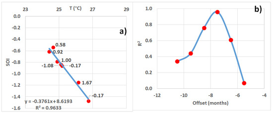
Figure 5.
(a) For every ENSO event inventoried in Table 1, the correlation between the minimum SOI filtered within the band of 1.5/15 years, and the monthly subsurface water temperature T at 2° S 180° W averaged over 125 to 175 m in depth, 7–8 months prior to the minimum SOI, is represented. The labels display the lag of the events (in years). (b) The coefficient of determination R2 versus the offset (the mean time elapsed prior to the minimum SOI).
During the period of observation extending from the end of 1993 to 2017, only one event was out of phase with the annual wave (lag = 1.00 year; see Table 1 and Figure 3). In this case, the ENSO event occurred while the annual component of the NECC flowed eastward. On the other hand, events that were unlagged or weakly and strongly lagged by referring to the quadrennial wave were well represented: two events were unlagged (lag = −0.17 years in both cases), two were weakly lagged (lag = 0.58 and 0.92 years), and two were strongly lagged (lag = −1.08 and 1.67 years).
The correlation over seven pairs T-SOI (Figure 5a) is highly dependent on the offset, that is, the elapsed time between the subsurface water temperature measurement and the ENSO, as shown in Figure 5b. It is optimal when the subsurface water temperature is measured between 7 and 8 months prior to when the ENSO is mature. So, a significant correlation is obtained when the temperature reaches its maximum. Since then, the maturation phase of the ENSO event is expected 7–8 months later, while the temperature gradually decreases (Figure 6).
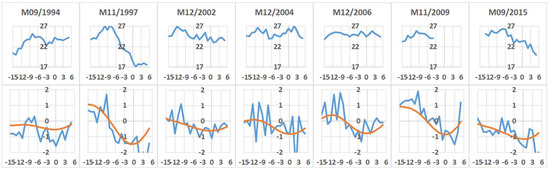
Figure 6.
The top plots represent the subsurface water temperature in °C at 2° S 180° W averaged over 125 to 175 m in depth versus the offset in months. The date of occurrence of the event corresponds to the null offset. The bottom plots depict the raw signal SOI (in blue) and that filtered within the band of 1.5/15 years (in red).
5. Discussion
Figure 4 suggests that the discharge of the warm water pool of the tropical Pacific in its western part and the transfer of warm water to the east induce a straightforward ocean-atmosphere interaction. In other words, convective processes in the upper ocean and in the low-level atmosphere are tightly controlled by the subsurface water temperature, whatever the amplitude or the date of occurrence of the resulting ENSO. The main deviation from this causal relationship of incredible simplicity appears when upwelling in the eastern Pacific is strongly stimulated during the westward phase propagation of the quadrennial QSW, so that the cold water that extends to the surface and generates nonlinear processes, leading to the amplification of the easterlies during La Niña recovery (Figure 4).
A first deduction can be made: if this exceptional circumstance is ignored, the ENSO can be characterized by the subsurface water temperature in the western Pacific without resorting to the SST in the central-eastern Pacific. However, the temperature of subsurface water in the western Pacific has no predictive value, as temperature and SOI fluctuations are concomitant. This temperature, which reflects the replacement of warm water by colder water, heralds the discharge of the warm water pool, which is in phase opposition with the SOI. Only the central-eastern part of the Pacific can provide information to anticipate the ENSO. It is clear from the linear relationship shown in Figure 5a that the ENSO, if characterized by the SOI, is based exclusively on the heat fluxes between the subsurface water of the central-eastern Pacific, and the atmosphere. These fluxes are therefore closely dependent on the vertical temperature gradient anomaly observed during warm events, both in the subsurface water and in the atmosphere, which in this case is related to the intensified moisture accumulation at low levels (e.g., [20]).
5.1. The Low-Level Atmosphere
During ENSO events, the tropical response of rain-producing cumulonimbus clouds is critical because deep convection is the principal agent for exchanging heat from the ocean’s surface to the free atmosphere. The effects of the ENSO on the circulation and convection during the Madden-Julian Oscillation (MJO) lifecycle [21] was studied by Tam and Lau [20], from both observations and the General Circulation Model (GCM), proving that the ENSO has a strong impact on MJO activity over the Pacific.
During warm events, the stronger magnitude of the instability index (measured by the vertical gradient of the anomalous moist static energy) over the central Pacific is conducive to more eastward penetration on convective anomalies in the region. Intra-seasonal variance of the low-level zonal flow is enhanced over the central-eastern Pacific, while it is suppressed over the western Pacific. The growth pattern associated with the MJO is found to be displaced eastward. There is also evidence that the phase speed of the MJO over the equatorial Pacific is reduced. These changes are mainly due to intensified moisture accumulation at low levels.
During cold events, smaller changes in this instability index are generally found and the convective anomalies stall in the western Pacific. However, as mentioned earlier, the cold water that extends to the surface may generate nonlinear processes, leading to the amplification of easterlies during La Niña recovery.
5.2. Inferences from the T-SOI Relationship
The great complexity of the convective processes occurring during warm events in both the ocean and the atmosphere is not reflected by phenomena of great regularity as they are considered globally at the basin scale. The linearity of the T-SOI relationship, observable in Figure 5a, of the pairs deduced from the seven ENSO events suggests the proportionality of:
- the increase in subsurface water temperature ∆T at 2° S 180° W averaged from 125 to 175 m in depth, 7–8 months prior to when the ENSO is mature;
- the increased mean heat flux in the central-eastern Pacific resulting from the induced convection processes while the thermocline of the quadrennial QSW is rising;
- the intensified moisture accumulation at low levels of the atmosphere over the central-eastern Pacific;
- the drop of atmospheric pressure at sea level between the central-eastern and the western Pacific that is considered to be representative of the Walker circulation, the minimum SOI occurring during the maturation phase of the ENSO.
Furthermore, there is a precise 7–8 month delay from the maximum subsurface water temperature at 2° S 180° W to the perturbation of low-level zonal flows over the central-eastern and the western Pacific (reflected by the SOI), whatever the amplitude or the date of occurrence of the resulting ENSO. These inferences form substantial elements of simplification in understanding the ENSO. On the other hand, they might constitute relevant information in dynamical models.
5.3. Impact of the ENSO on Climate
5.3.1. Highlighting Atmospheric Baroclinic Waves from Precipitation
In the tropics, heat transfer from the Pacific Ocean to the atmosphere produces quasi-geostrophic motion of the atmosphere [22]. From the heating zone are formed equatorial-trapped eastward Kelvin waves and westward Rossby waves; hence, easterly trade winds are set up by atmospheric Kelvin waves to the east and westerlies occur as an atmospheric planetary wave response to the west.
The impact of the ENSO can be evidenced from the variability of precipitation height, as are the equatorial atmospheric baroclinic waves. The latter are forced by deep convection to the troposphere which is enhanced over very warm sea surfaces in the tropics, altering the vertical density profile. These inertial waves, which arise from the difference in density between the lower and upper layers of the atmosphere, result in the oscillation of the upper layers of the troposphere. The baroclinic wave modes do vary in the vertical: they alternatively induce precipitations or drier conditions depending on the lapse rate, that is, the altitude of warm and wet layers in the upper troposphere.
In order to eliminate the seasonal variability, the raw daily data (averaged over a month) of the ENSO-influenced precipitation are averaged over annual periods framing the ENSO maturation phase, that is, when the filtered SOI signal in the 1.5/15 year band reaches a minimum. Then, the ratio of the mean annual precipitation, impacted by particular ENSO events, to the annual precipitation averaged over the whole period of observation is represented at the planetary scale. The selection of particular events allows distinguishing the 4-year rainfall oscillation at mid-latitudes from the remote impact of the ENSO [23].
Four new events are considered when comparing the SOI/RH (Rainfall Height) over the period of 1979–2017: two are out of phase with the annual QSW (lag = −0.75 and 1.33 years), one is weakly lagged (lag = 0.92 years), and one is strongly lagged (lag = 1.92 years), as shown in Table 2.
Table 2.
Four new events are considered when comparing the SOI/RH (Rainfall Height).
5.3.2. Events Out of Phase with the Annual QSW
An important cause of variability of ENSO events is the time lag. This parameter reflects how the eastward phase propagation of the quadrennial QSW occurs in the central-eastern Pacific. Four types of events can be characterized by the lag according to whether they are unlagged, weakly, or strongly lagged, or out of phase with the annual QSW. Actually, unlagged and weakly lagged events behave in a similar way. The number of these observed events is not sufficient to highlight any specific features pertaining exclusively to their time lag. So, only three types of events are the subject of this comparative study of their impact according to whether they are (1) unlagged or weakly lagged, (2) strongly lagged, or (3) out of phase with the annual QSW.
Although of less importance than the time lag, another cause of variability of the impact of ENSO events is their amplitude. In general, the higher the amplitude, the greater the impact. Also, the few events of very small amplitude cannot contribute to specify their typology.
Figure 7 displays the impact of the ENSO from the variability of precipitation height in the case of events out of phase for which heat transfer from the ocean to the atmosphere occurs both in the central and eastern tropical Pacific, that is, what is commonly named central Pacific (CP) events as opposed to eastern Pacific (EP) events. However, we will avoid using this terminology later, as it tends to be reductive. Two significant events are considered, which occurred in May 1987 (lag = 1.33 years, SOI = −0.91) and December 2006 (lag = 1.00 year, SOI = −0.79). These events induce an eastward-propagating atmospheric Kelvin wave of high amplitude recognizable by abundant precipitations all along a narrow band over the equatorial Pacific. The Kelvin wave retains its shape as it moves along the equator over time, although it broadens during its progression far from the central Pacific. On the other hand, a westward-propagating Rossby wave in the opposite phase is recognizable by low precipitations in the western Pacific.
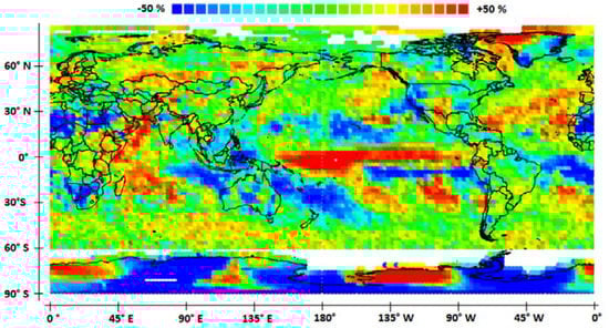
Figure 7.
Impact of the ENSO from the variability of precipitation height (the deviation is expressed in % compared to the average precipitation). To each class corresponds an equivalent area within the band 30° S–30° N (quantiles of the total area). The precipitation scale is roughly linear between the two extreme classes (here, −50% and 50%). However, the two extreme classes include precipitation heights equal to or higher/lower than what is indicated. ENSO events out of phase with the annual QSW are considered.
The apparent wavelength of the atmospheric Kelvin wave is around 25,000 km, meaning that it impacts both the equatorial Pacific and the eastern Indian Ocean between 30° S and 30° N where the increase in precipitation may reach 50%. In contrast, precipitation is reduced in the tropical Atlantic Ocean. The Kelvin wave has a considerable impact at the planetary scale, producing remote impacts of El Niño in locations such as Antarctica and California that suffer from severe drought conditions. These events are characterized by a significant contribution, in the maturation phase, of heat transfers between latitudes 5° N and 20° N in the central Pacific resulting from the northern antinode of the annual QSW [13]. Such events are lagged due to the coupling between the annual and the quadrennial QSWs. When it is lagged, the quadrennial QSW may interact strongly and transiently with the annual QSW during the eastward phase propagation, while the modulated currents at the northern node of the annual QSW and at the main node of the quadrennial QSW flow in opposite directions during the second half of the year. This enhances heat transfers at the northern antinode of the annual QSW while delaying by half a year the eastward propagation of the quadrennial QSW.
The atmospheric Rossby wave, which is in the opposite phase compared to the Kelvin wave, impacts Southeast Asia and Oceania while sparing Australia, with the decrease in precipitation possibly reaching 50%.
5.3.3. Unlagged and Weakly Lagged Events
Figure 8 displays the impact of the ENSO in the case of unlagged and weakly lagged events for which heat transfer from the ocean to the atmosphere mainly occurs in the eastern tropical Pacific. Five significant events are considered, which occurred in December 1982 (lag = 0.92 years, SOI = −1.83), September 1994 (lag = 0.58 years, SOI = −0.54), November 1997 (lag = −0.17 years, SOI = −1.48), December 2002 (lag = 0.92 years, SOI = −0.62), and November 2009 (lag = −0.17 years, SOI = −0.86).
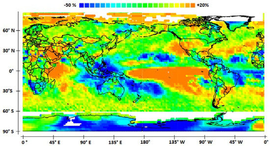
Figure 8.
Impact of the ENSO from the variability of precipitation height. Unlagged and weakly lagged events are considered.
The amplitude of the atmospheric Kelvin wave is much lower than that in the previous case, with the relative deviation of rainfall height rarely overreaching 20%. Regions remotely impacted are the same except Antarctica, which is affected very little, and California, which is subject to abundant rainfall. As a result of the Rossby wave, impacted regions in the western Pacific are more extended. Now, they include Australia and probably Antarctica between 90° W and 170° W, as indicated by the comparison of Figure 7 and Figure 8.
5.3.4. Strongly Lagged Events
Figure 9 displays the impact of the ENSO from the variability of precipitation height in the case of strongly lagged events for which heat transfer from the ocean to the atmosphere also mainly occurs in the eastern tropical Pacific, but geostrophic forces are less favorable to the eastward propagation of the quadrennial QSW than in the preceding case. Three significant events are considered, which occurred in December 1991 (lag = 1.92 years, SOI = −0.86), January 2005 (lag = −1.08 years, SOI = −0.84), and September 2015 (lag = 1.67 years, SOI = −1.15).
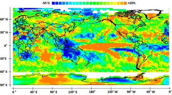
Figure 9.
Impact of the ENSO from the variability of precipitation height. Strongly lagged events are considered.
The amplitude of the atmospheric Kelvin wave looks similar to the previous case, with the relative deviation of rainfall height again rarely overreaching 20%, but the impacted regions are smaller. In particular, the Arabic peninsula is weakly influenced. Concerning the atmospheric Rossby wave, the impacted regions are the same, with a strong amplification of droughts in Australia and South Africa. On the other hand, the impact of the ENSO on western South America reverses, creating drought conditions in Peru, probably amplified owing to the rapid restoration of La Niña in early 2016. Finally, the remote impact on Antarctica seems considerably lessened compared to previous events, but this does not necessarily result from the ENSO, as this continent is currently affected by various influences.
5.3.5. Some Suggestions about the Strong Impact of Events out of Phase with the Annual QSW
As shown in Figure 7, the amplitude of the Kelvin wave is considerable when events out of phase with the annual QSW occur, which raises some questions. Some authors have proposed answers to this problem. Kim et al. [24] suggested that the generation of this type of ENSO event may be linked to extratropical forcing associated with the North Pacific Oscillation (NPO). However, observations from precipitations tend to show that, as already observed in the tropical oceans, the atmospheric planetary waves respond strongly to thermal sources and sinks because of quasi-resonance when the period of forcing coincides with their natural period. For this to happen, the apparent wavelength of equatorial atmospheric waves must adapt to approach the resonance conditions by favoring some modes of baroclinic waves. When this condition is fulfilled, resonantly forced waves exert their prominence over non-resonant waves, for which forcing is less efficient, which may ensure their stability. This topic warrants further discussed.
5.4. Implementation of the Prediction Method
Virtually, the prediction of warm events can be performed as soon as the monthly subsurface water temperature at 2° S 180° W averaged over 125 to 175 m in depth reaches a maximum (Figure 10). However, although attenuated, the peaks corresponding to the annual QSW have to be distinguished from the peaks resulting from the eastward phase propagation of the quadrennial QSW (Figure 10). Only the latter anticipate ENSO events. No clue allows distinguishing the origin of the subsurface water temperature peaks at 2° S 180° W unless they are compared to those of the subsurface water at both ends of the western antinode of the quadrennial QSW. These are the geostrophic forces at the tropical basin scale that cause Kelvin waves to be generated from off-equatorial Rossby waves in the extreme western Pacific, or not. In particular, these forces are governed by the tilt along the equator of the SSH [11].
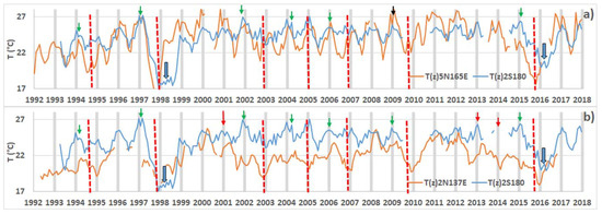
Figure 10.
(a) The top plot represents the monthly subsurface water temperature at 5° N 165° E averaged over 100 to 150 m in depth and at 2° S 180° W averaged over 125 to 175 m in depth. (b) The bottom plot represents the subsurface water temperature at 2° N 137° E averaged over 100 to 200 m in depth and at 2° S 180° W averaged over 125 to 175 m in depth. Dashed red lines indicate the maturation phase of ENSO events. Green arrows depict harbingers of ENSO events; red arrows depict false harbingers detected and the black arrow denotes a true harbinger that was rejected. Thick arrows show the temperature drop during the intensification of La Niña. Peaks occurring during the maturation phase of ENSO events are ignored since they necessarily concern the annual QSW (two successive ENSO events are separated by at least 1.5 years). It should be noted that seasonal forecasting centers predicted an El Niño for 2012, while it should have occurred in early 2013.
Geostrophic forces occurring in the tropical basin can be materialized by considering the subsurface water temperature at particular locations of the western off-equatorial antinodes nearly in the opposite phase with respect to the central-eastern antinode. Indeed, as displayed in Figure 4, the subsurface water temperature at 2° N 137° E averaged over 100 to 200 m in depth, which is located at the western antinode close to the most westerly limit of the tropical basin, reflects the raising of the pycnocline depth as the westward-propagating off-equatorial Rossby waves are deflected off the western boundary of the basin to form a train of eastward-propagating Kelvin waves guided by the equator. At this location, the thermocline should reflect the discharge of the warm water pool of the tropical Pacific in its western part and the transfer of warm water to the east. This is actually achieved when the subsurface water temperatures at both locations, that is, 2° N 137° E and 2° S 180° W (the most westerly tip of the central-eastern antinode of the quadrennial QSW), are close. Nevertheless, as shown if Figure 10b, the subsurface water temperature at 2° N 137° E does not allow the unambiguous discrimination of the origin of the peaks because the temperature curve associated with the quadrennial QSW may decrease while being overlaid on a peak resulting from the annual QSW, as occurred in 2001, 2012, and 2014. In these cases, the geostrophic forces in the central-eastern tropical basin disable the eastward propagation of the equatorial-trapped Kelvin waves. Consequently, the Kelvin waves remain confined in the western part of the basin and no ENSO event is trigged. Especially striking is the behavior of the thermocline in 2012 and 2014, which suggested that an ENSO event was maturing while that was not the case [8,9].
More selective information can be inferred from the subsurface water temperature at the most easterly tip of the western antinode of the quadrennial QSW located in the northern hemisphere, that is, at 5° N 165° E (Figure 2 and Figure 10a). Peaks of the subsurface water temperature at 2° S 180° W are relevant when they are higher than the subsurface water temperature at 5° N 165° E, proving that the off-equatorial antinode is entirely involved in the transfer of warm water. However, some peaks may be rejected while resulting from the quadrennial QSW, as occurred in 2009 (Figure 10a). Thus, the use of both information delivered at 2° N 137° E and at 5° N 165° E is required to recognize the peaks resulting from the quadrennial QSW exhaustively and unambiguously. Actually, the peaks may be acknowledged with certainty in all cases (Figure 10a) except when deductions are contradictory, as occurred in 2009. In that particular case, only a probabilistic approach is relevant.
When a peak is acknowledged to have resulted from the quadrennial QSW, a linear relationship (Figure 5a) allows an estimation of the amplitude of the event that will occur 7–8 months later. Thereby, such an estimation of the date of occurrence of the ENSO is straightforward and certainly more accurate than that used to demonstrate the feasibility of the method by filtering the SOI signal, which is of no practical use.
The peaks of the subsurface water temperature at 2° S 180° W resulting from the annual and quadrennial QSWs do not overlap, which explains the simple linear relationship of the T-SOI pairs. This suggests that the southernmost antinode of the annual QSW located in the northern hemisphere, as well as the northernmost antinode located in the southern hemisphere, deviate from the path of the quadrennial QSW during its eastward phase propagation while its central-eastern antinode is growing.
As concerns the cold events, the amplification of La Niña can be seen a few months before the maturation phase of the ENSO event, as happened in 1998 and 2016, when the subsurface water temperature at 2° S 180° W dropped (Figure 10). Such a decrease in temperature observed at the beginning of the westward phase propagation of the quadrennial QSW is a harbinger of upwelling amplification in the eastern Pacific and the development of a high atmospheric pressure system.
6. Conclusions
The study of resonantly forced baroclinic waves in the tropical Pacific allowed us to lift part of the veil on the ENSO phenomenology. Furthermore, by ignoring the unique signature of ENSO events in the SST lifecycle, concrete information was deduced from this new approach, improving the ability to accurately forecast ENSO events.
The peaks of the subsurface water temperature measured in the central-eastern antinode of the quadrennial QSW at 2° S 180° W either reflect the annual QSW or the quadrennial QSW distinctly, without any overlap. The peaks resulting from the quadrennial QSW are recognizable by comparing them to the subsurface water temperature at both ends of the western antinode in the northern hemisphere. This allows predicting the date of occurrence as well as the amplitude of warm ENSO events 7–8 months prior to their maturation phase by using the linear relationship of T-SOI.
By not taking into account the SST explicitly, the prevision of warm ENSO events (amplitude, date of occurrence, impacted regions according to the lag) is straightforward. This apparent simplicity reflects that, between the central-eastern and the western Pacific, the ocean-atmosphere interactions in the central-eastern Pacific induce a strong coherence between the subsurface water temperatures and the atmospheric pressure drop at sea level.
The prevision of cold events has to consider that upwelling in the eastern Pacific may be strongly stimulated during the westward phase propagation of the quadrennial QSW, which may considerably strengthen the La Niña resumption, as occurred at the end of 1998 and 2016. Such events can be anticipated a few months before the maturation phase of the ENSO event from the drop in the subsurface water temperature.
The prediction of the climate impact of ENSO involves the time lag of the events that reflects their modes of variability. Like the date of occurrence, the time lag is forecasted 7–8 months prior to the maturation phase. Two main types of events can be distinguished according to whether the quadrennial QSW is in phase or not with the annual QSW. The dephasing of both QSWs leads to what is commonly named central Pacific (CP) events. However, when both QSWs are in phase, the characteristics of the resulting eastward Pacific (EP) events can be nuanced according to whether they are (1) unlagged or weakly lagged, or (2) strongly lagged. The coherence of both QSWs has considerable climatic consequences because of their quasi-resonant forcing effect on atmospheric Kelvin waves. By categorizing events according to their time lag, their impact is predictable several months in advance.
Funding
This research received no external funding.
Acknowledgments
We thank the associated editor and the reviewers for their helpful comments.
Conflicts of Interest
The author declares no conflict of interest.
References
- Yang, S.; Jiang, X. Prediction of eastern and central Pacific ENSO events and their impacts on east Asian climate by the NCEP climate forecast system. J. Clim. 2014, 27, 4451–4472. [Google Scholar] [CrossRef]
- Imada, Y.; Tatebe, H.; Ishii, M.; Chikamoto, Y.; Mori, M.; Arai, M.; Watanabe, M.; Kimoto, M. Predictability of two types of El Niño assessed using an extended seasonal prediction system by MIROC. Mon. Weather Rev. 2015, 143, 4597–4617. [Google Scholar] [CrossRef]
- Jin, E.K.; Kinter, J.L.; Wang, B.; Park, C.-K.; Kang, I.-S.; Kirtman, P.B.; Kug, J.-S.; Kumar, A.; Luo, J.-J.; Schemm, J.; et al. Coauthors Current status of ENSO prediction skill in coupled ocean–atmosphere models. Clim. Dyn. 2008, 31, 647–664. [Google Scholar] [CrossRef]
- Zebiak, S.E. Oceanic heat content variability and El Niño cycles. J. Phys. Oceanogr. 1989, 19, 475–486. [Google Scholar] [CrossRef]
- Meinen, C.S.; McPhaden, M.J. Observations of warm water volume changes in the equatorial Pacific and their relationship to El Niño and La Niña. J. Clim. 2000, 13, 3551–3559. [Google Scholar] [CrossRef]
- Kumar, A.; Wen, C.; Xue, Y.; Wang, H. Sensitivity of Subsurface Ocean Temperature Variability to Specification of Surface Observations in the Context of ENSO. In Monthly Weather Review; American Meteorological Society: Boston, MA, USA, 2017; Volume 145, No. 4. [Google Scholar]
- Barnston, A.G.; Tippett, M.K.; L'Heureux, M.L.; Li, S.; DeWitt, D.G. Skill of Real-Time Seasonal ENSO Model Predictions during 2002–2011: Is Our Capability Increasing? Bull. Am. Meteorol. Soc. 2012, 93, 631–651. [Google Scholar] [CrossRef]
- McPhaden, M.J. Playing hide and seek with El Niño. Nat. Clim. Chang. 2015, 5, 791–795. [Google Scholar] [CrossRef]
- McPhaden, M.J.; Timmermann, A.; Widlansky, M.J.; Balmaseda, M.A.; Stockdale, T.N. The Curious Case of the EL Niño That Never Happened: A Perspective from 40 Years of Progress in Climate Research and Forecasting. Bull. Am. Meteorol. Soc. 2015, 96, 1647–1665. [Google Scholar] [CrossRef]
- Smith, N.; Kessler, W.S.; Hill, K.; Carlson, D. Progress in Observing and Predicting ENSO. 2015, Volume 64. Available online: https://public.wmo.int/en/resources/bulletin/progress-observing-and-predicting-enso-0 (accessed on 30 May 2018).
- Pinault, J.L. Long wave resonance in tropical oceans and implications on climate: The Pacific Ocean. Pure Appl. Geophys. 2015, 173, 2119–2145. [Google Scholar] [CrossRef]
- Choi, M.Y.; Thouless, D.J. Topological interpretation of sub-harmonic mode locking in coupled oscillators with inertia. Phys. Rev. B 2001, 64. [Google Scholar] [CrossRef]
- Trenberth, K. The definition of El Niño. Bull. Am. Meteorol. Soc. 1997, 78, 2771–2777. [Google Scholar] [CrossRef]
- Pinault, J.L. Anticipation of ENSO: What teach us the resonantly forced baroclinic waves. Geophys. Astrophys. Fluid Dyn. 2016, 110, 518–528. [Google Scholar] [CrossRef]
- Explain with Realism Climate Variability. Available online: http://climatorealist.neowordpress.fr/el-nino/ (accessed on 11 March 2018).
- Davey, M.K.; Brookshaw, A.; Ineson, S. The probability of the impact of ENSO on precipitation and near-surface temperature. Clim. Risk Manag. 2014, 1, 5–24. [Google Scholar] [CrossRef]
- Meyers, G.; Donguy, J.R. An XBT network with merchant ships. Trop. Ocean Atmos. Newslett. 1980, 2, 6–7. [Google Scholar]
- Wyrtki, K. The subsurface water masses in the western South Pacific Ocean. Aust. J. Mar. Freshw. Res. 1962, 13, 18–48. [Google Scholar] [CrossRef]
- Wyrtki, K. El Niño-The dynamic response of the equatorial Pacific Ocean to atmospheric forcing. J. Phys. Oceanogr. 1975, 5, 572–584. [Google Scholar] [CrossRef]
- Tam, C.-Y.; Lau, N.-C. Modulation of the Madden-Julian Oscillation by ENSO: Inferences from Observations and GCM Simulations. J. Meteorol. Soc. Jpn. 2005, 83, 727–743. [Google Scholar] [CrossRef]
- Madden, R.A.; Julian, P.R. Detection of a 40–50 day oscillation in the zonal wind in the tropical Pacific. J. Atmos. Sci. 1971, 28, 702–708. [Google Scholar] [CrossRef]
- Gill, A.E. Atmosphere–Ocean Dynamics. In International Geophysics Series; Academic Press: Cambridge, MA, USA, 1982; Volume 30, p. 662. [Google Scholar]
- Pinault, J.L. Regions Subject to Rainfall Oscillation in the 5–10 Year band. Climate 2018, 6, 2. [Google Scholar] [CrossRef]
- Kim, S.T.; Yu, J.-Y.; Kumar, A.; Wang, H. Examination of the Two Types of ENSO in the NCEP CFS Model and Its Extratropical Associations. In Monthly Weather Review; American Meteorological Society: Boston, MA, USA, 2012; Volume 140, No. 6. [Google Scholar]
© 2018 by the author. Licensee MDPI, Basel, Switzerland. This article is an open access article distributed under the terms and conditions of the Creative Commons Attribution (CC BY) license (http://creativecommons.org/licenses/by/4.0/).