1. Introduction
The degradation of underwater images quality is mainly attributed to light scattering and absorption. The light is attenuated as it propagates through water and the attenuation varies according to the wavelength of light within the water column depth and depends also on the distance of the objects from the point of view. The suspended particles in the water are also responsible for light scattering and absorption. In many cases, the image taken underwater seems to be hazy, in a similar way as it happens in landscape photos degraded by haze, fog or smoke, which also cause absorption and scattering. Moreover, as the water column increases, the various components of sunlight are differently absorbed by the medium, depending on their wavelengths. This lead to a dominance of blue/green colour in the underwater imagery that is known as colour cast. The visibility can be increased and the colour can be recovered by using artificial light sources in an underwater imaging system. But artificial light does not illuminate the scene uniformly and it can produce bright spots in the images due to the backscattering of light in the water medium.
The work presented in this paper is part of the i-MARECULTURE project [
1,
2,
3] that aims to develop new tools and technologies for improving the public awareness about underwater cultural heritage. In particular, it includes the development of a Virtual Reality environment that reproduces faithfully the appearance of underwater sites, giving the possibility to visualize the archaeological remains as they would appear in air. This goal requires a comparison of the different image enhancement algorithms to figure out which one performs better in different environmental and illumination conditions. We selected five algorithms from the state of the art and we used them to enhance a dataset of images produced in various underwater sites at heterogeneous conditions of depth, turbidity and lighting. These enhanced images have been evaluated by means of some quantitative metrics. There are several different metrics known in scientific literature employed to evaluate underwater enhancement algorithms, so we have chosen only three of them to complete our evaluation.
2. State of the Art
The problem of underwater image enhancement is closely related to the single image dehazing in which images are degraded by weather conditions such as haze or fog. A variety of approaches have been proposed to solve image dehazing and, in this section, we are reporting their most effective examples. Furthermore, we’re also reporting the algorithms that address the problem of non-uniform illumination in the images and others that focus on colour correction.
Single image dehazing methods assume that only the input image is available and rely on image priors to recover a dehazed scene. One of the most cited works on single image dehazing is the dark channel prior (DCP) [
4]. It assumes that, within small image patches, there will be at least one pixel with a dark colour channel and uses this minimal value as an estimate of the present haze. This prior achieves very good results in some context, except in bright areas of the image where the prior does not hold. In [
5] an extension of DCP to deal with underwater image restoration is presented. Based on the consideration that the red channel is often nearly dark in underwater images due to preferential absorption of different colour wavelengths in the water, this new prior, called Underwater Dark Channel Prior (UDCP), considers just the green and the blue colour channels in order to estimate the transmission. An author mentioned many times in the field is Fattal, R and his two works [
6,
7]. In the first work [
6] Fattal et al. formulate a refined image formation model that accounts for surface shading in addition to the transmission function. This allows for resolving ambiguities in data by searching for a solution in which the resulting shading and transmission functions are statistically uncorrelated. The second work [
7] describes a new method for single-image dehazing that relies on a generic regularity in natural images, where pixels of small image patches typically present a one-dimensional distribution in RGB colour space, known as colour-lines. Starting from this consideration, Fattal et al. derive a local formation model that explains the colour-lines in the context of hazy scenes and use it for recovering the scene transmission based on the offset of the lines from the origin. Another work focused on lines of colour in the hazy image is presented in [
8,
9]. The authors describe a new prior for single image dehazing that is defined as a Non-Local prior, to underline that the pixels forming the lines of colour are spread across the entire image, thus capturing a global characteristic that is not limited to small image patches.
Some other works focus on the problem of non-uniform illumination that, in the case of underwater imagery, is often produced by the artificial light needed at the deepest point. The work proposed in [
10] suggests a method for non-uniform illumination correction for underwater images. The method assumes that natural underwater images are Rayleigh distributed and uses maximum likelihood estimation of scale parameters to map distribution of image to Rayleigh distribution. In [
11] is presented a simple gradient domain method that acts as a high pass filter, aimed to correct the effect of non-uniform illumination and preserve the image details. A simple prior which estimates the depth map of the scene considering the difference in attenuation among the different colour channels is proposed in [
12]. The scene radiance is recovered from the hazy image through the estimated depth map by modelling the true scene radiance as a Markov Random Field.
Bianco et al. have presented in [
13] the first proposal for colour correction of underwater images by using lαβ colour space. A white balancing is performed by moving the distributions of the chromatic components (α, β) around the white point and the image contrast is improved through a histogram cut-off and stretching of the luminance (l) component. In [
14,
15] is proposed a method for unsupervised colour correction of general purpose images. It employs a computational model that is inspired on some adaptation mechanisms of the human vision to realize a local filtering effect by taking into account the colour spatial distribution in the image.
Finally, we report a state of the art method that is effective in image contrast enhancement, since underwater images often lack in contrast. This is the Contrast Limited Adaptive Histogram Equalization (CLAHE) proposed in [
16] and summarized in [
17], which was originally developed for medical imaging and has proven to be successful for enhancing low-contrast images.
3. Selected Algorithms
In order to perform our evaluation, we have selected five algorithms that perform well and employ different approaches for the resolution of the underwater image enhancement problem, such as image dehazing, non-uniform illumination correction and colour correction. The decision to select these algorithms among all the other is based on a preliminary brief evaluation of their enhancement performance. Furthermore, we selected these algorithms also because we could find for them a trusty implementation done by the authors of the papers or by a reliable author. Indeed, we need such an implementation to develop the software tool we employed to speed-up the benchmark and that will be useful for further images processing and evaluation. The source codes of all the selected algorithms have been adapted and merged in the tool. We employed the OpenCV [
18] library for the tool development in order to exploit its functions for images managing and processing.
3.1. Automatic Colour Enhancement (ACE)
The ACE algorithm is a quite complex technique, due to its direct computation on an N × N image costs
operations. For this reason, we have followed the approach proposed in [
19] that describes two fast approximations of ACE. First, an algorithm that uses a polynomial approximation of the slope function to decompose the main computation into convolutions, reducing the cost to
Second, an algorithm based on interpolating intensity levels that reduces the main computation to convolutions too. In our test, ACE was processed using the level interpolation algorithm with 8 levels. Two parameters that can be adjusted to tune the algorithm behaviour are α and the weighting function
The α parameter specifies the strength of the enhancement: the larger this parameter, the stronger the enhancement. In our test, we used the standard values for this parameter, e.g., α = 5 and
. For the implementation, we used the ANSI C source code referred in [
19] that we adapted in our enhancement tool (
supplementary materials).
3.2. Contrast Limited Adaptive Histogram Equalization (CLAHE)
The CLAHE [
16,
17] algorithm is an improved version of AHE, or Adaptive Histogram Equalization. Both are aimed to improve the standard histogram equalization. CLAHE was designed to prevent the over amplification of noise that can be generated using the adaptive histogram equalization. CLAHE partitions the image into contextual regions and applies the histogram equalization to each of them. Doing so, it balances the distribution of used grey values in order to make hidden features of the image more evident. We implemented this algorithm in our enhancement tool employing the CLAHE function provided by the OpenCV library. The input images are converted in lαβ colour space and then the CLAHE algorithm is applied only on the luminance (l) channel. OpenCV provide two parameters in order to control the output of this algorithm: the tile size and the contrast limit. The first parameter is the size of each tile in which the original image is partitioned and the second one is a parameter useful to limit the contrast enhancement in each tile. If noise is present, it will be amplified as well. So, in noisy images, such as underwater images, it should be better to limit the contrast enhancement to a low value, in order to avoid the amplification of noise. In our test, we set tile size at 8 × 8 pixels and contrast limit to 2.
3.3. Colour Correction Method on lαβ Space (LAB)
This method [
13] is based on the assumptions of grey world and uniform illumination of the scene. The idea behind this method is to convert the input image form RGB to LAB space, correct colour casts of an image by adjusting the α and β components, increasing contrast by performing histogram cut-off and stretching and then convert the image back to the RGB space. The author provided us with a MATLAB implementation of this algorithm but, due to the intermediate transformations of colour space, needed to convert the input image from RGB to LAB and due to the lack of optimization of the MATLAB code, this implementation was very time-consuming. Therefore, we managed to port this code in C++ by employing OpenCV among other libraries. This enabled us to include this algorithm in our enhancement tool and to decrease the computing time by an order of magnitude.
3.4. Non-Local Image Dehazing (NLD)
The basic assumption of this algorithm is that colours of a haze-free image can be well approximated by a few hundred distinct colours. These few colours can be grouped in tight colour clusters in RGB space. The pixels that compose a cluster are often located at different positions across the image plane and at different distances from the camera. So, each colour cluster in the clear image becomes a line in RGB space of a hazy image, at which the authors refer to as a hazy-line. By means of these haze-lines, this algorithm recovers both the distance map and the dehazed image. The algorithm is linear in the size of the image and the authors have published an official MATLAB implementation [
20]. In order to include this algorithm in our enhancement tool, we have conducted a porting in C++, employing different library as OpenCV, Eigen [
21] for the operation on sparse matrix not supported by OpenCV and FLANN [
22] (Fast Library for Approximate Nearest Neighbours) to compute the colour cluster.
3.5. Screened Poisson Equation for Image Contrast Enhancement (SP)
The output of the algorithm is an image which is the result of applying the Screened Poisson equation [
11] to each colour channel separately, together with a simplest colour balance [
23] with a variable percentage of saturation as parameter (s). The Screened Poisson equation can be solved by using the discrete Fourier transform. Once found the solution in Fourier domain, the application of the discrete inverse Fourier transform yields the result image. The simplest colour balance is applied both before and after the Screened Poisson equation solving. The complexity of this algorithm is
. The ANSI C source code is provided by the authors in [
11] and we adapted it in our enhancement tool. For the Fourier transform, this code relies on the library FFTw [
24]. The algorithm output can be controlled with the trade-off parameter α and the level of saturation of the simplest colour balance s. In our evaluation, we used as parameters
.
4. Case Studies
We tried to produce a dataset of images that was as heterogeneous as possible, in order to better represent the variability of environmental and illumination conditions that characterizes underwater imagery. Furthermore, we choose images taken with different cameras and with different resolutions, because in the real application cases the underwater image enhancement algorithms have to deal with images produced by unspecific sources. In this section, we describe the underwater sites, the dataset of images and the motivations that lead us to choose them.
4.1. Underwater Sites
Four different sites have been selected on which the images for the evaluation of the underwater image enhancement algorithms were taken. The selected sites are representative of different states of environmental and geomorphologic conditions (i.e., water depth, water turbidity, etc.).
Two of them are pilot sites of the i-MARECULTURE project, the Underwater Archaeological Park of Baiae and the Mazotos shipwreck. The other two are the Cala Cicala and Cala Minnola shipwrecks.
4.1.1. Underwater Archaeological Park of Baiae
The Underwater Archaeological Park of Baiae is located off the north-western coasts of the bay of Puteoli (Naples). This site has been characterized by a periodic volcanic and hydrothermal activity and it has been subjected to gradual changes in the levels of the coast with respect to the sea level. The Park safeguards the archaeological remains of the Roman city that are submerged at a depth ranging between 1 and 14–15 m below sea level. This underwater site is usually characterized by a very poor visibility because of the water turbidity, which in turn is mainly due to the organic particles suspended in the medium. So, the underwater images produced here are strongly affected by the haze effect [
25].
4.1.2. Mazotos Shipwreck
The second site is the Mazotos shipwreck that lies at a depth of 44 m, ca.14 nautical miles (NM) southwest of Larnaca, Cyprus, off the coast of Mazotos village. The wreck lies on a sandy, almost flat seabed and consists of an oblong concentration of at least 800 amphorae, partly or totally visible before any excavation took place. The investigation of the shipwreck is conducted jointly by the Maritime Research Laboratory (MARE Lab) of the University of Cyprus and the Department of Antiquities, under the direction of Dr Stella Demesticha. Some 3D models of the site have been created by using photogrammetric techniques [
26]. The visibility in this site is very good but the red absorption at this depth is nearly total, so the images were taken using an artificial light for recovering the colour.
4.1.3. Cala Cicala
In 1950, near Cala Cicala, within the Marine Protected Area of Capo Rizzuto (Province of Crotone, Italy), the archaeological remains of a large Roman Empire ship were discovered at a depth of 5 m. The so-called Cala Cicala shipwreck, still set for sailing, carried a load of raw or semi-finished marble products of considerable size. In previous work, the site has been reconstructed with 3D photogrammetry and it can be enjoyed in Virtual Reality [
27]. The visibility in this site is good.
4.1.4. Cala Minnola
The underwater archaeological site of Cala Minnola is located on the East coast of the island of Levanzo, in the archipelago of the Aegadian Islands, few miles from the west coast of Sicily. The site preserves the wreck of a Roman cargo ship at a depth from the sea level ranged from 25 m to 30 m [
28]. The roman ship was carrying hundreds of amphorae which should have been filled with wine. During the sinking, many amphorae were scattered across the seabed. Furthermore, the area is covered by large seagrass beds of Posidonia. In this site, the visibility is good but, due to the water depth, the images taken here suffer from serious colour cast because of the red channel absorption and, therefore, they appear bluish.
4.2. Image Dataset
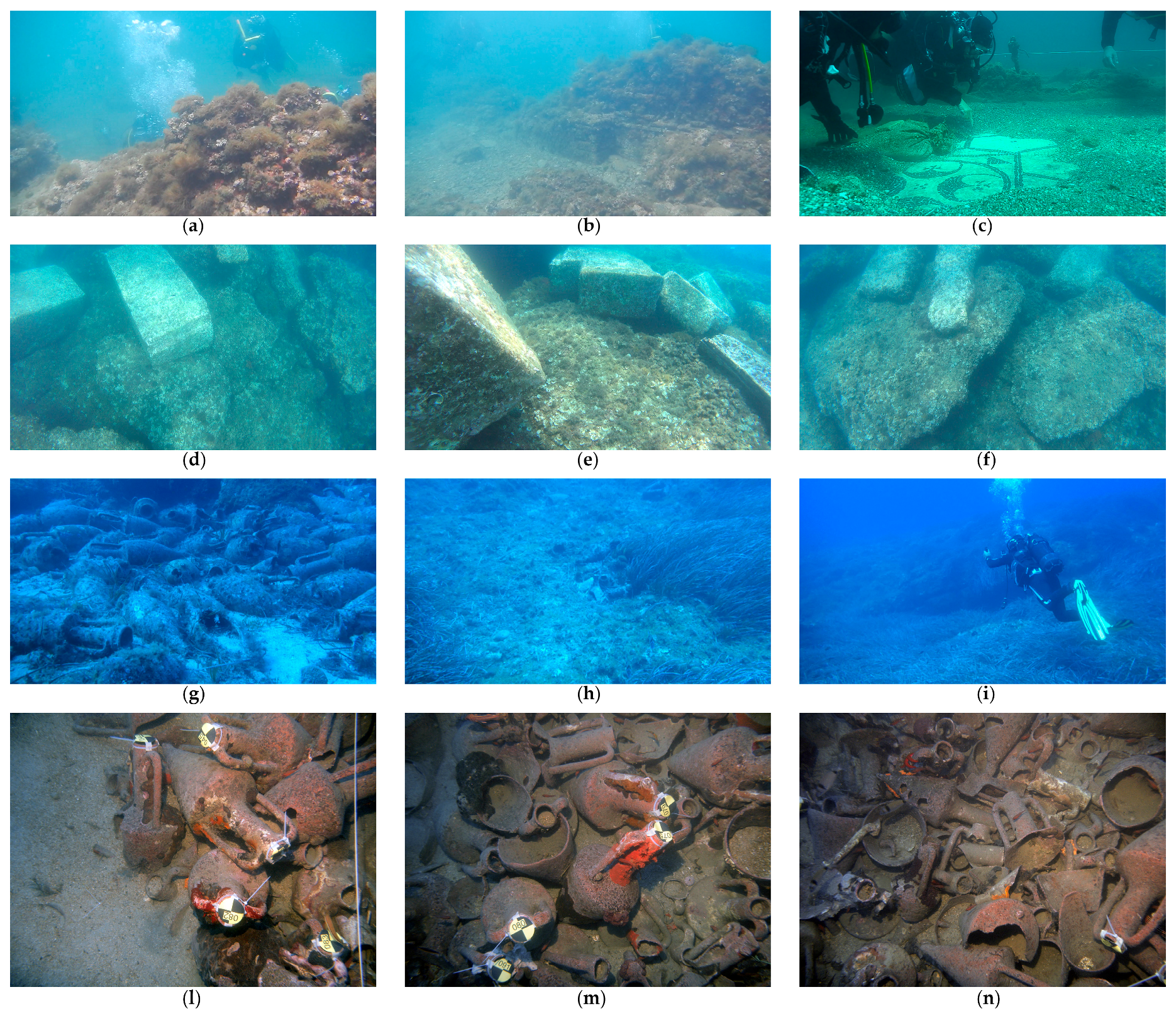
For each underwater site described in the previous section, we selected three representative images for a total of twelve images. These images constitute the underwater dataset that we employed to complete our evaluation of image enhancement algorithms.
Each row of the
Figure 1 represents an underwater site. The properties and modality of acquisition of the images vary depending on the underwater site. In the first row (a–c) we can see the images selected for the Underwater Archaeological Park of Baiae that, due to the low water depth, are naturally illuminated. The first two (a,b) were acquired with a Nikon Coolpix, a non-SLR (Single-Lens Reflex) camera, at a resolution of 1920 × 1080 pixels. The third image (c) was taken with a Nikon D7000 DSLR (Digital Single-Lens Reflex) camera with a 20 mm f/2.8 lens and have the same resolution of 1920 × 1080 pixels. The second row (d–f) shows three images of some semi-finished marble from the Cala Cicala shipwreck. They were acquired with natural illumination using a Sony X1000V, a 4 K action camera, with a resolution of 3840 × 2160 pixels. In the third row (g–i) we can see the amphorae of a Roman cargo ship and a panoramic picture, all taken at the underwater site of Cala Minnola. These images were acquired with an iPad Air and have a resolution of 1920 × 1080 pixels. Despite of the depth of this underwater site, these pictures were taken without artificial illumination and so they look bluish. Therefore, these images are a challenge for understanding how the selected underwater algorithms can deal with such a situation to recover the colour cast. In the last row we can find the pictures of the amphorae at the Mazotos shipwreck. Due to the considerable water depth, these images were acquired with an artificial light, using a Canon PowerShot A620, a non-SLR camera, with a resolution of 3072 × 2304 pixels that implicates an image ratio of 4:3, different from the 16:9 ratio of the images taken at the other underwater sites. The use of artificial light to acquire these images had produced a bright spot due to the backward scattering.
The described dataset is composed by very heterogeneous images that address a wide range of potential underwater environmental conditions and problems, as the turbidity in the water that make the underwater images hazy, the water depth that causes colour casting and the use of artificial light that can lead to bright spots. It makes sense to expect that each of the selected image enhancement algorithms should perform better on the images that represent the environmental conditions against which it was designed.
5. Evaluation Methods
Each image included in the dataset described in the previous section was processed with each of the image enhancement algorithm introduced in the
Section 3, taking advantage of the enhancement processing tool that we developed including all the selected algorithms in order to speed up the processing task. The authors suggested some standard parameters for their algorithms in order to obtain good enhancing results. Some of these parameters could be tuned differently in the various underwater conditions in order to improve the result. We decided to let all the parameters with the standard values in order not to influence our evaluation with a tuning of the parameters that could have been more effective for an algorithm than for an another.
We have employed some quantitative metrics, representative of a wide range of metrics employed in the field of underwater image enhancement, to evaluate all the enhanced images. In particular, these metrics are employed in the evaluation of hazy images in [
29]. Similar metrics are defined in [
30] and employed in [
10]. So, the objective performance of the selected algorithms is evaluated in terms of the following metrics. The first one is obtained by calculating the mean value of image brightness. Formally, it’s defined as
where
,
is the intensity value of the pixel
in the colour channel
,
denotes
row and
column,
and
L denotes the total number of rows and columns respectively. When
is smaller, the efficiency of image dehazing is better. The mean value on the three colour channels is a simple arithmetic mean
.
Another metric is the information entropy, that represent the amount of information contained in the image. It is expressed as
where
denotes the distribution probability of the pixels at intensity level
. An image with the ideal equalization histogram possesses the maximal information entropy of 8 bit. So, the bigger the entropy, the better the enhanced image. The mean value on the three colour channels is defined as
The third metric is the average gradient of the image which represents the local variance among the pixels of the image, so bigger its value better the resolution of the image. It’s defined as:
where
is the intensity value of the pixel
in the colour channel
,
denotes
row and
column,
and
L denote the total number of rows and columns, respectively. The mean value on the three colour channels is a simple arithmetic mean
.
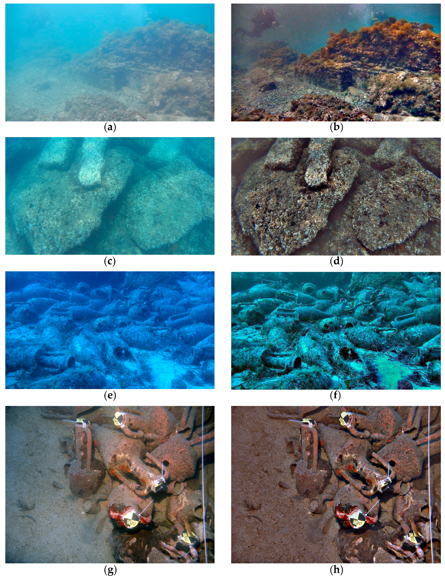
6. Results
This section reports the results of the quantitative evaluation performed on all the images in the dataset, both for the original ones and for the ones enhanced with each of the previously described algorithms. The dataset is composed by twelve images. So, enhancing them with the five algorithms, the total of the images to be evaluated with the quantitative metrics is 72 (12 originals and 60 enhanced). For practical reasons, we will report here only a sample of our results, that consists of the original image named as “Baia1” and its five enhanced versions (
Figure 2).
Table 1 contains the results of quantitative evaluation performed on the images showed in
Figure 2. The first column reports the metric values for the original images and the following columns report the correspondent values for the images enhanced with the concerning algorithms. Each row, instead, reports the value of each metric calculated for each colour channel and its mean value, as defined in
Section 5. The values marked in bold correspond to the best value for the metric defined by the corresponding row. Focusing on the mean values of the three metrics (
), it can be deduced that the SP algorithm performed better on the mean brightness, the ACE algorithm performed better on enhancing the information entropy and the CLAHE algorithm improved more than the others the average gradient. So, according to these values, these three algorithms in this case of the “Baia1” sample image gave qualitatively equal outcomes. Perhaps it’s possible to deduce another consideration by analysing the value of the metrics for the single colour channels. In fact, looking at all the values marked in bold, the SP algorithm reached better results more times than the other two. So, the SP algorithms should have performed slightly better in this case.
For each image in the dataset we have elaborated a table such as
Table 1. Since it is neither practical nor useful to report here all these tables, we summarized them in a single table (
Table 2).
The
Table 2 has four sections, one for each underwater site. Each of these sections reports the average values of the metrics calculated for the related site and defined as
where (
), (
), (
) are the metrics calculated for the first, the second and the third sample image of the related site, respectively. Obviously, the calculation of these metrics was carried out on the three images enhanced by each algorithm. In fact, each column reports the metrics related to a given algorithm.
This table enables us to deduce some more global considerations about the performances of the selected algorithms on our images dataset. Focusing on the values in bold, we can deduce that the SP algorithm has performed better in the sites of Baiae, Cala Cicala and Cala Minnola, having totalized the higher values in two out of three metrics (. Moreover, looking at the entropy (, i.e., the metric on which SP has lost, we can recognize that the values calculated for this algorithm are not so far from the values calculated for the other algorithms. As regards the underwater site of Mazotos, the quantitative evaluation conducted with these metrics seems not to converge on any of the algorithms. Moreover, the ACE algorithm seems to be the one that performs better in enhancing the information entropy of the images.
For the sake of completeness, we want to report a particular case that is worth mentioning. Looking at
Table 3, it’s possible to conclude that the SP algorithm performed better than all the others according to all the three metrics in the case of “CalaMinnola2.”
In
Figure 3 we can see the CalaMinnola2 image enhanced with the SP algorithm. It’s quite clear, looking at this image, that the SP algorithm in this case have generated some ‘artefacts,’ likely due to the oversaturation of some image details. This issue could be probably solved or attenuated by tuning the saturation parameter of the SP algorithm, which we have fixed to a standard value, as for the parameters of the other algorithms too. Anyway, the question is that the metrics were misled by this ‘artefacts,’ assigning a high value to the enhancement made by this algorithm.
7. Conclusions
In this work, we have selected five state-of-the-art algorithms for the enhancement of images taken on four underwater sites with different environmental and illumination conditions. We have evaluated these algorithms by means of three quantitative metrics selected among those already adopted in the field of underwater image enhancement. Our purpose was to establish which algorithm performs better than the others and whether or not the selected metrics were good enough to compare two or more image enhancement algorithms.
According to the quantitative metrics, the SP algorithm seemed to perform better than the other in all the underwater sites, except for Mazotos. For this site, each metric assigned a higher value to a different algorithm, preventing us to decide which algorithm performed better on the Mazotos images. Such an undefined result is the first drawback to evaluate the underwater images relying only on quantitative metrics. Moreover, these quantitative metrics, implementing only a blind evaluation of a specific intrinsic characteristic of the image, are unable to identify ‘problems’ in the enhanced images, as the ‘artefacts’ generated by the SP algorithms in the case documented in
Figure 3 and
Table 3.
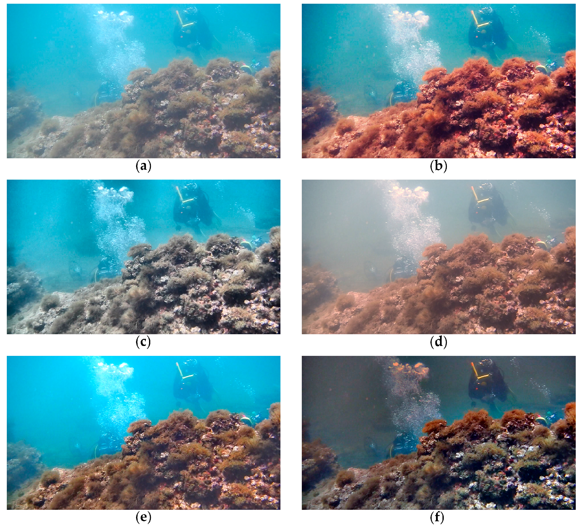
Anyway, looking at
Figure 4 and performing a qualitative analysis from the point of view of the human perception, the result suggested by the quantitative metrics seems to be confirmed, as the SP algorithm performed well in most of the cases. The only case on which the SP algorithms failed was in the Cala Minnola underwater site, probably due to an oversaturation of some image details that probably could be fixed by tuning its saturation parameter.
In conclusion, even if the quantitative metrics can provide a useful indication about image quality, they do not seem reliable enough to be blindly employed for an objective evaluation of the performances of an underwater image enhancement algorithm. Hence, in the future we intend to design an alternative methodology to evaluate the underwater image enhancement algorithms. Our approach will be based on the judgement of a panel of experts in the field of underwater imagery, that will express an evaluation on the quality of the enhancement conducted on an underwater images dataset through some selected algorithms. The result of the expert panel judgement will be used as reference in the algorithms evaluation, comparing it to the results obtained through a larger set of quantitative metrics that we will select from the state of the art. We will conduct this study on a wider dataset of underwater images that will be more representative of the underwater environment conditions.


