Comparative Analysis of Coastal Flooding Vulnerability and Hazard Assessment at National Scale

 ,
,  ,
, 
Abstract
1. Introduction
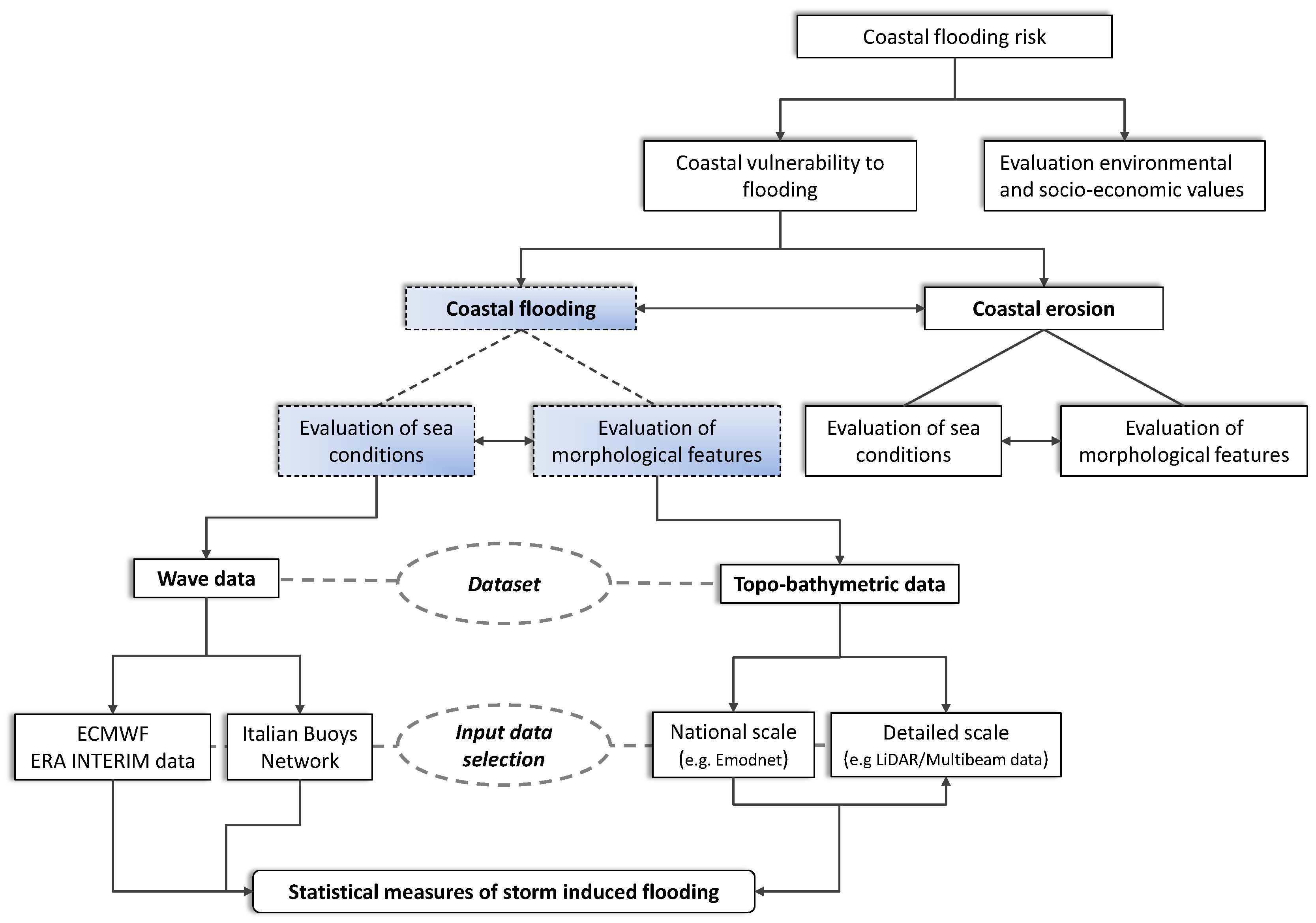
2. Methods
- nearshore wave conditions;
- wave runup;
- Coastal Vulnerability Index;
- Coastal Hazard Index
2.1. Nearshore Wave Conditions
2.2. Wave Runup
2.3. Coastal Vulnerability Index and Coastal Hazard Index
3. The Case Study of Montalto Di Castro
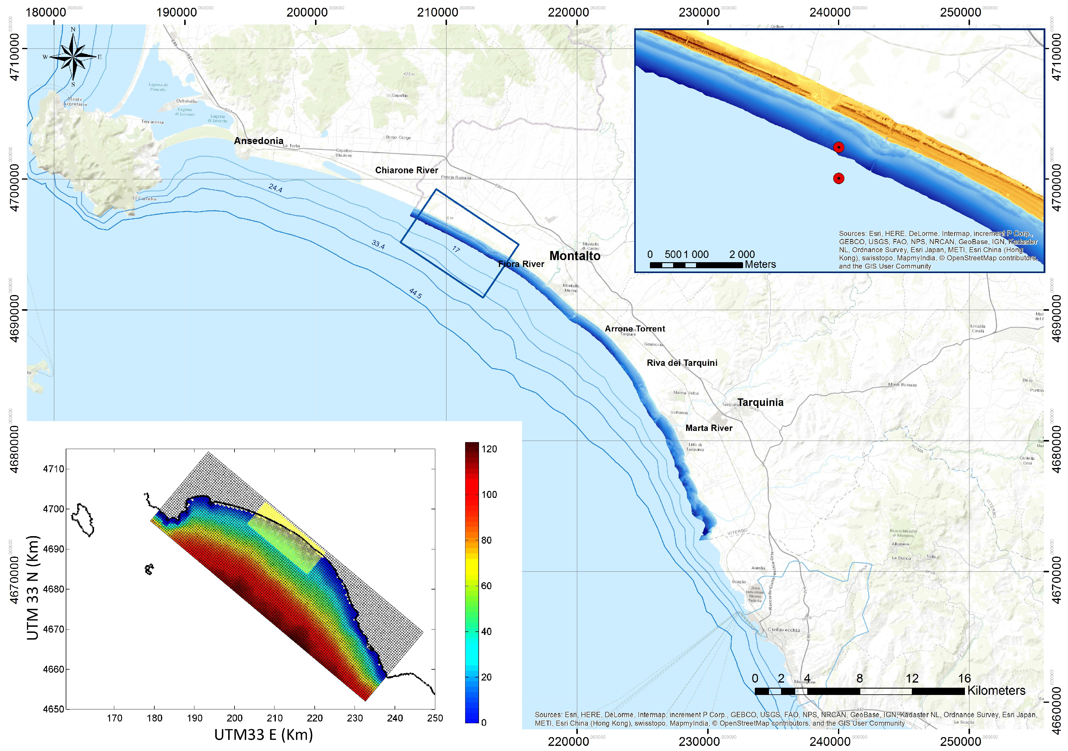
3.1. Site Description
3.2. Data
4. Results and Discussion
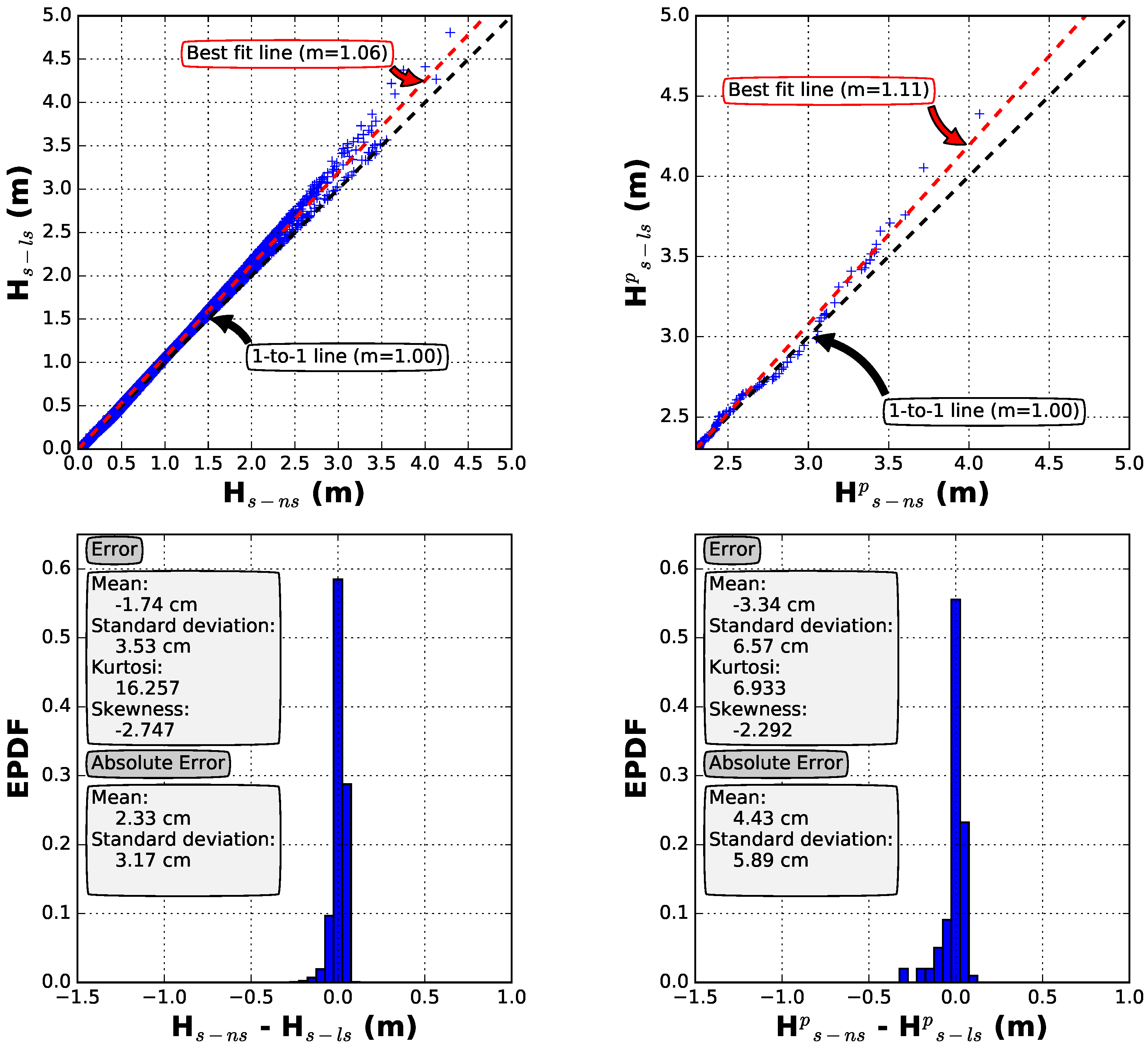
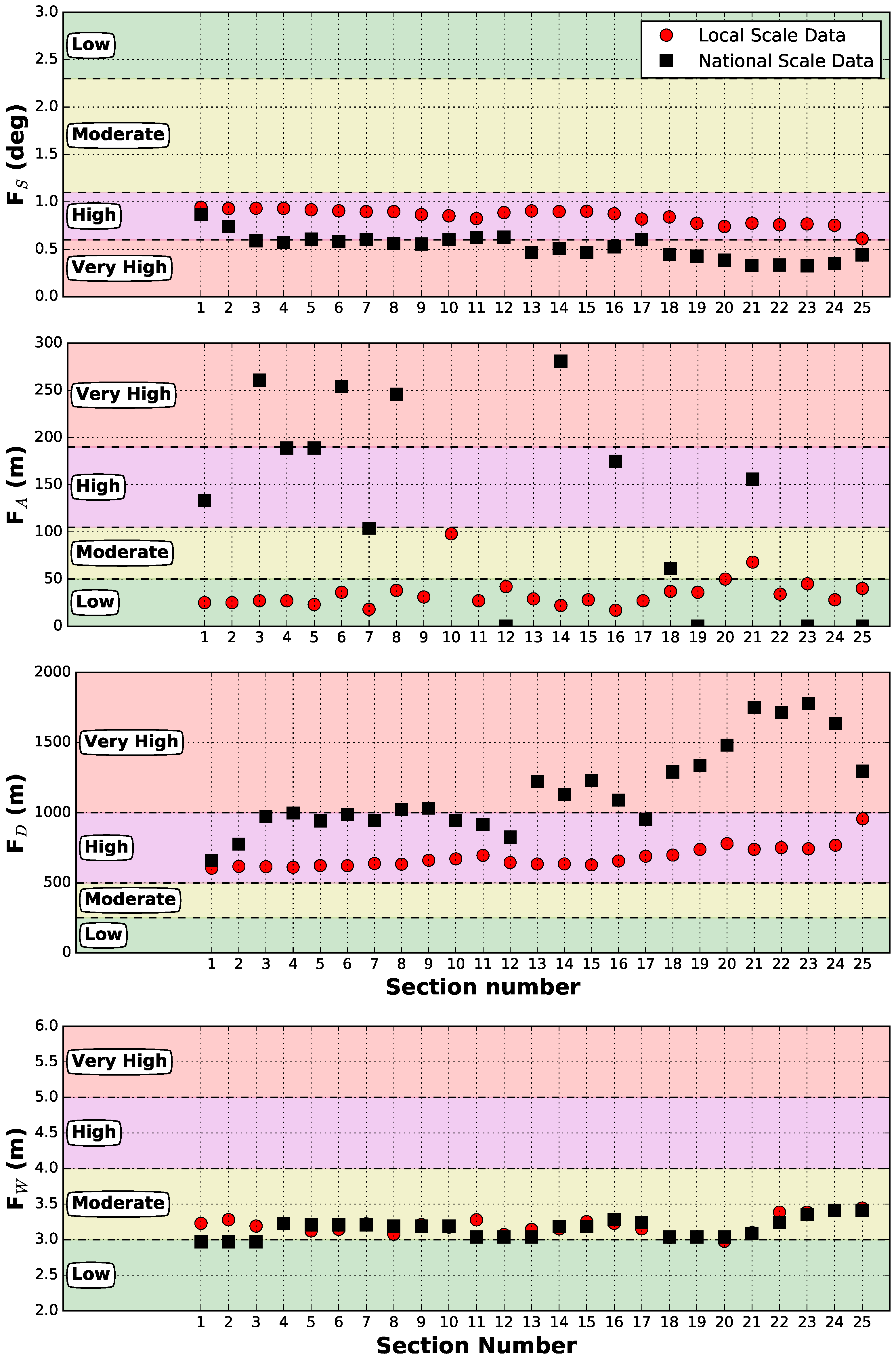
4.1. Nearshore Wave Parameters
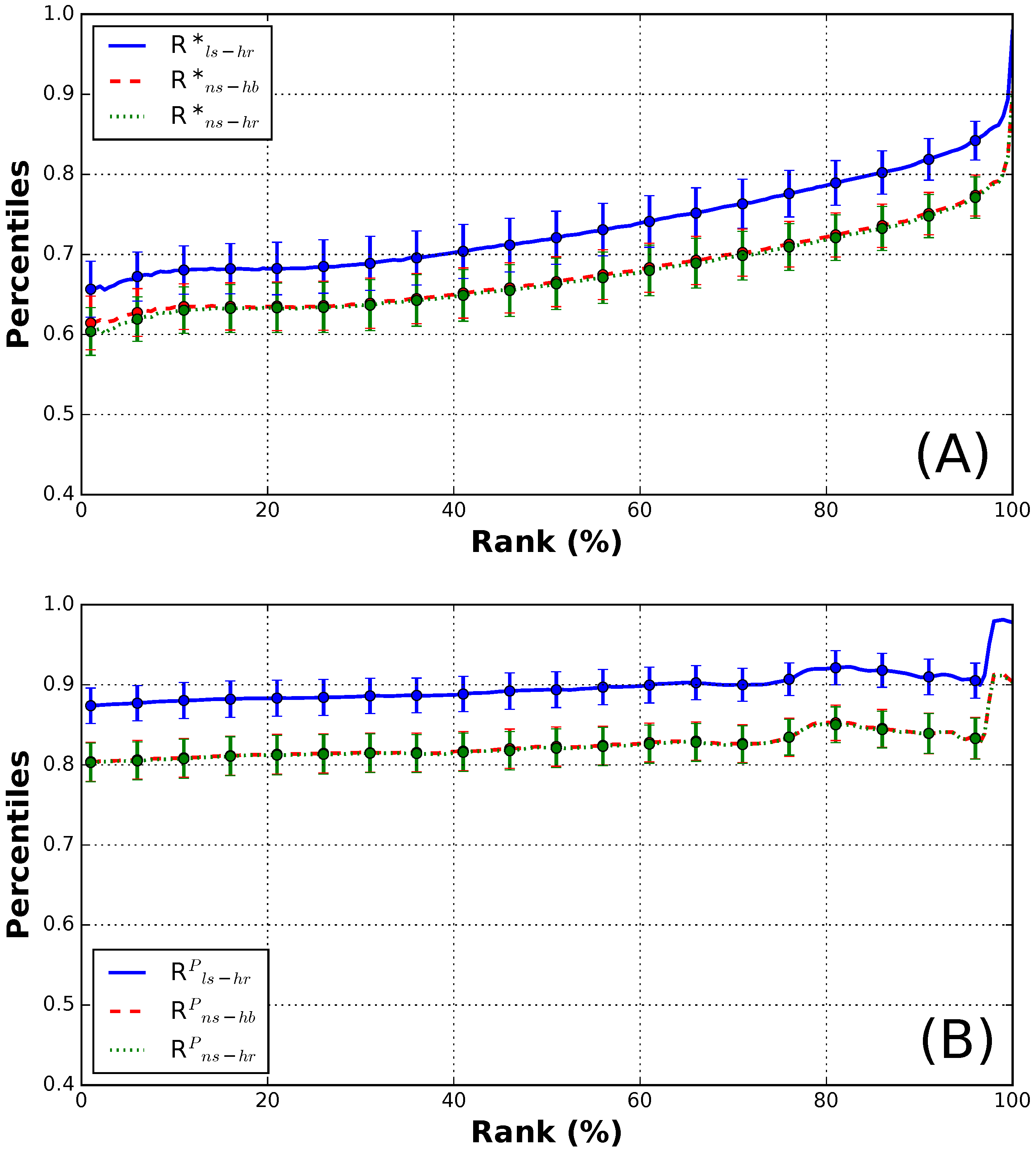
4.2. Wave Runup
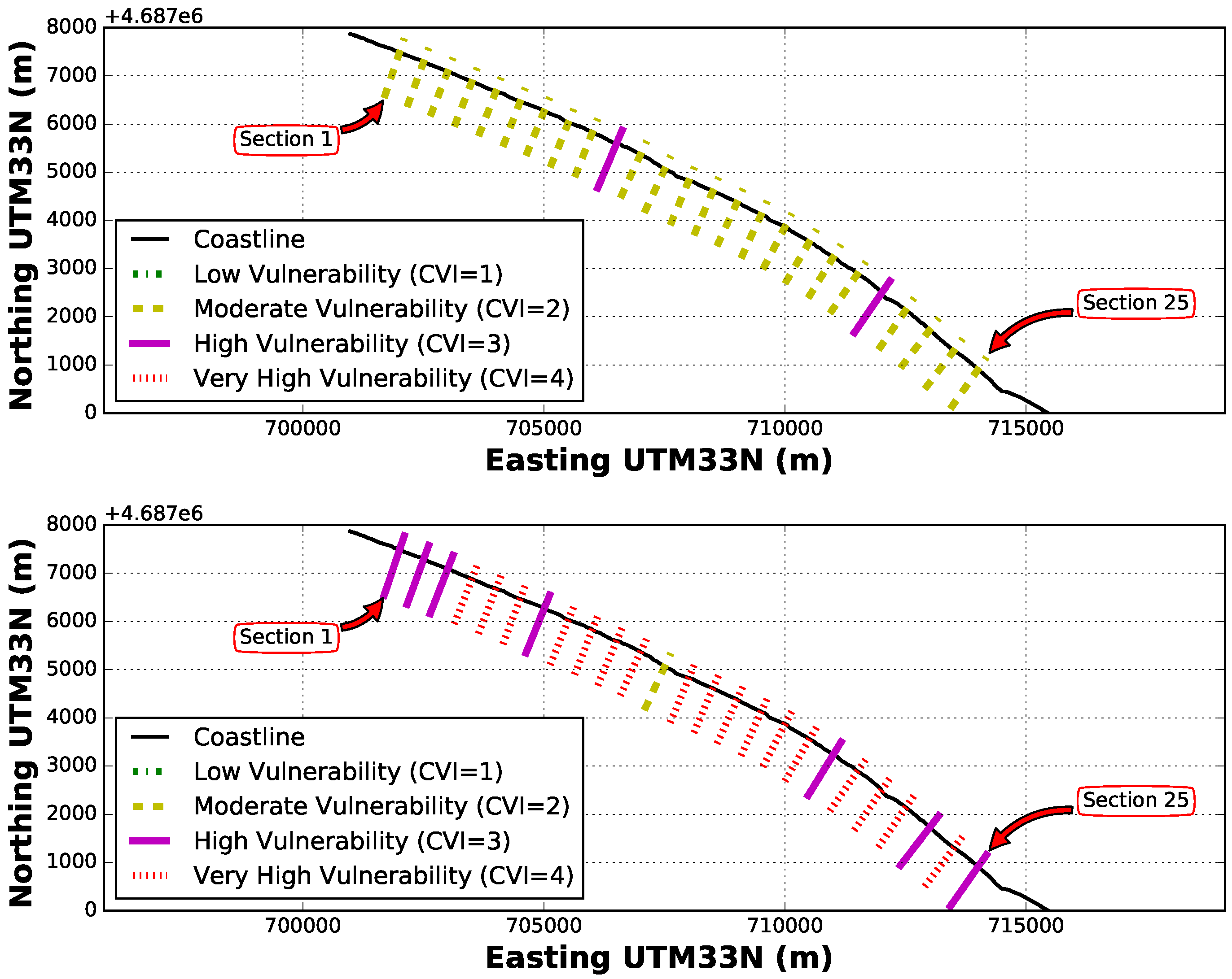
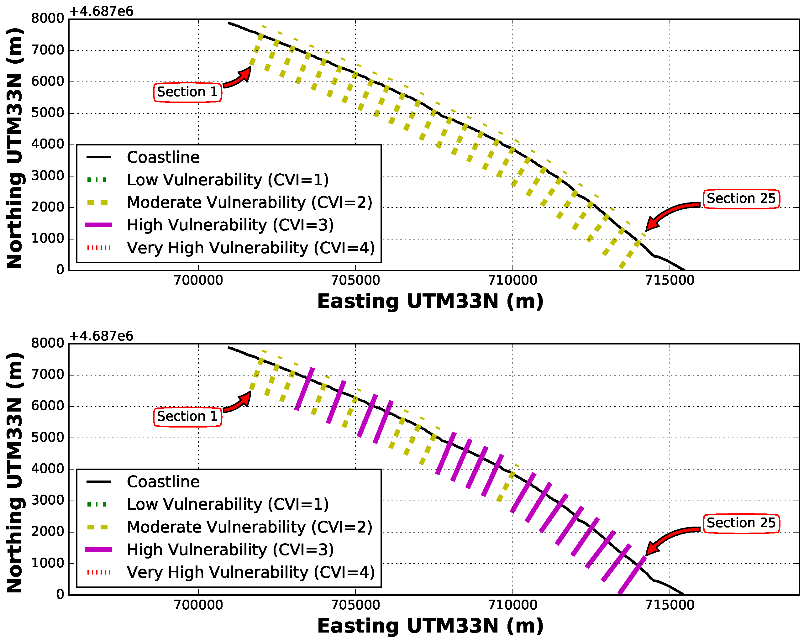
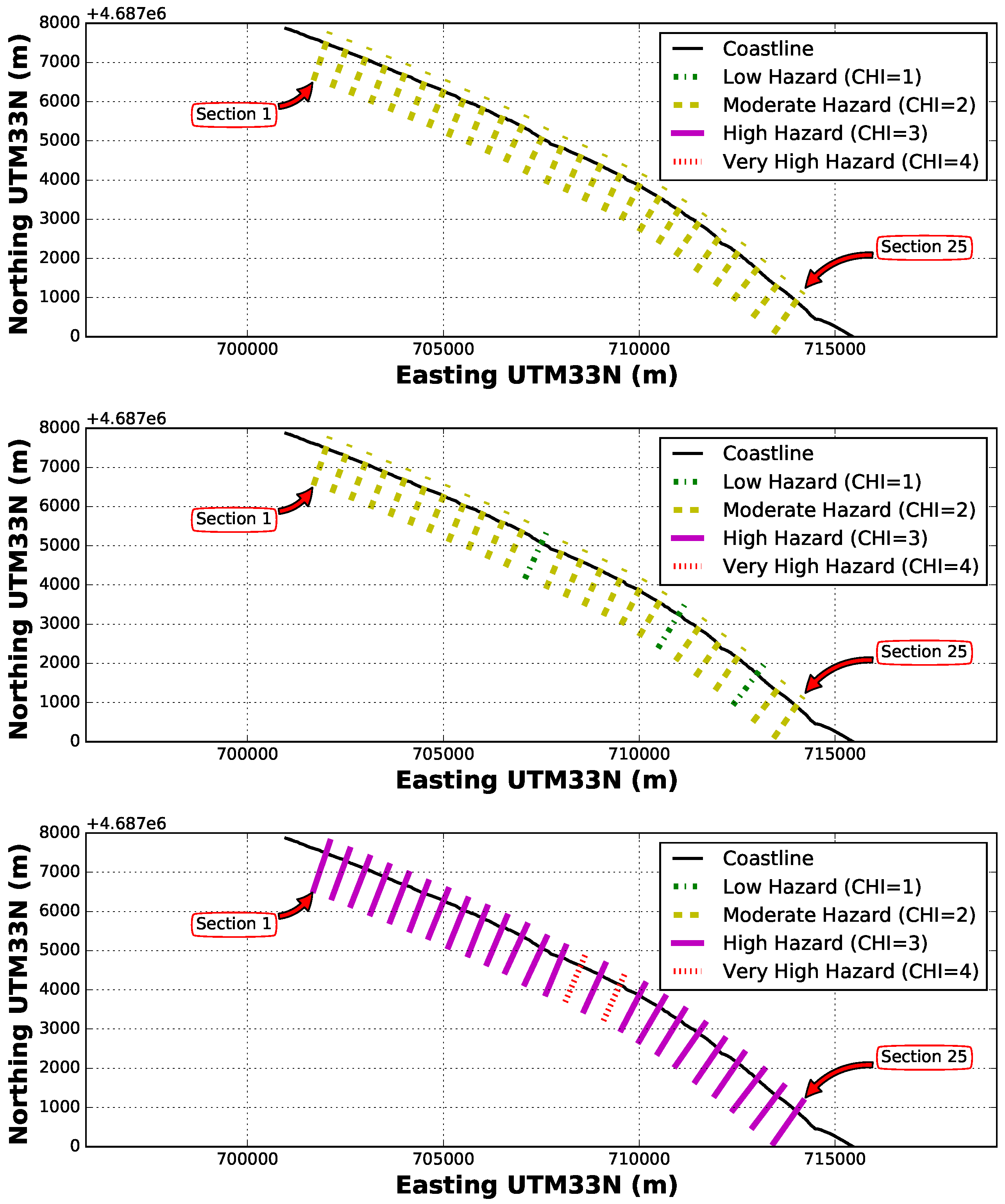
4.3. Coastal Vulnerability Index and Coastal Hazard Index
5. Concluding Remarks and Ongoing Research
Acknowledgments
Author Contributions
Conflicts of Interest
References
- Meur-Férec, C.; Deboudt, P.; Morel, V. Coastal risks in France: An integrated method for evaluating vulnerability. J. Coast. Res. 2008, 24, 178–189. [Google Scholar] [CrossRef]
- Ciavola, P.; Armaroli, C.; Perini, L.; Luciani, P. Evaluation of maximum storm wave run-up and surges along the Emilia-Romagna coastline (NE Italy): A step towards a risk zonation in support of local CZM strategies. In Integrated Coastal Zone Management-The Global Challenge; Kannen, A., Ramanathan, A., Glavovic, B.C., Green, D.R., Krishnamurthy, R.R., Tinti, S., Agardy, T., Han, Z., Eds.; Research Publishing Services: Oxford, UK, 2008; Chapter 16; pp. 505–516. [Google Scholar]
- De Girolamo, P.; Di Risio, M.; Romano, A.; Molfetta, M. Landslide Tsunami: Physical Modeling for the Implementation of Tsunami Early Warning Systems in the Mediterranean Sea. Procedia Eng. 2014, 70, 429–438. [Google Scholar] [CrossRef]
- Perini, L.; Calabrese, L.; Salerno, G.; Ciavola, P.; Armaroli, C. Evaluation of coastal vulnerability to flooding: Comparison of two different methodologies adopted by the Emilia-Romagna region (Italy). Nat. Hazards Earth Syst. Sci. 2016, 16, 181–194. [Google Scholar] [CrossRef]
- Spaulding, M.L.; Grilli, A.; Damon, C.; Crean, T.; Fugate, G.; Oakley, B.A.; Stempel, P. STORMTOOLS: coastal environmental risk index (CERI). J. Mar. Sci. Eng. 2016, 4, 54. [Google Scholar] [CrossRef]
- Nageswara Rao, K.; Subraelu, P.; Venkateswara Rao, T.; Hema Malini, B.; Ratheesh, R.; Bhattacharya, S.; Rajawat, A.S.; Ajai. Sea-level rise and coastal vulnerability: An assessment of Andhra Pradesh coast, India through remote sensing and GIS. J. Coast. Conserv. 2008, 12, 195–207. [Google Scholar] [CrossRef]
- Di Risio, M.; Lisi, I.; Beltrami, G.; De Girolamo, P. Physical modeling of the cross-shore short-term evolution of protected and unprotected beach nourishments. Ocean Eng. 2010, 37, 777–789. [Google Scholar] [CrossRef]
- Mendoza, E.T.; Ojeda, E.; Meyer-Arendt, K.J.; Salles, P.; Appendini, C.M. Assessing Coastal Vulnerability in Yucatan (Mexico). Coast. Manag. 2016, 607–616. [Google Scholar] [CrossRef]
- Tapsell, S.; McCarthy, S.; Faulkner, H.; Alexander, M. Social Vulnerability to Natural Hazards; CapHaz-Net WP4 Report; Flood Hazard Research Centre—FHRC, Middlesex University: London, UK, 2010. [Google Scholar]
- Silva, S.F.; Martinho, M.; Capitão, R.; Reis, T.; Fortes, C.J.; Ferreira, J.C. An index-based method for coastal-flood risk assessment in low-lying areas (Costa de Caparica, Portugal). Ocean Coast. Manag. 2017, 144, 90–104. [Google Scholar] [CrossRef]
- De Bruijn, K.; Klijn, F.; Ölfert, A.; Penning-Rowsell, E.; Simm, J.; Wallis, M. Flood Risk Assessment and Flood Risk Management; An Introduction and Guidance Based on Experiences and Findings of FLOODsite (An EU-Funded Integrated Project); T29-09-01; FLOODsite Consortium: Wallingford, UK, 2009. [Google Scholar]
- Gornitz, V.M.; Daniels, R.C.; White, T.W.; Birdwell, K.R. The development of a coastal risk assessment database: vulnerability to sea-level rise in the US Southeast. J. Coast. Res. 1994, 327–338. [Google Scholar]
- De Moel, H.; van Alphen, J.; Aerts, J.C.J.H. Flood maps in Europe: Methods, availability and use. Nat. Hazards Earth Syst. Sci. 2009, 9, 289–301. [Google Scholar] [CrossRef]
- Archetti, R.; Paci, A.; Carniel, S.; Bonaldo, D. Optimal index related to the shoreline dynamics during a storm: The case of Jesolo beach. Nat. Hazards Earth Syst. Sci. 2016, 16, 1107–1122. [Google Scholar] [CrossRef]
- La Valle, P.; Paganelli, D.; Ercole, S.; Lisi, I.; Teofili, C.; Nicoletti, L. Coastal Management and Environmental Guidelines Related to Coastal Defence Works. In Changing Coast, Changing Climate, Changing Minds; ICE Publishing: London, UK, 2016; pp. 69–75. [Google Scholar]
- Torresan, S.; Critto, A.; Dalla Valle, M.; Harvey, N.; Marcomini, A. Assessing coastal vulnerability to climate change: Comparing segmentation at global and regional scales. Sustain. Sci. 2008, 3, 45–65. [Google Scholar] [CrossRef]
- Hinkel, J.; Klein, R.J. Integrating knowledge to assess coastal vulnerability to sea-level rise: The development of the DIVA tool. Glob. Environ. Chang. 2009, 19, 384–395. [Google Scholar] [CrossRef]
- Ciavola, P.; Ferreira, O.; Dongeren, A.V.; Vries, J.V.T.D.; Armaroli, C.; Harley, M. Prediction of Storm Impacts on Beach and Dune Systems. In Hydrometeorological Hazards: Interfacing Science and Policy, 1st ed.; Philippe, Q., Ed.; John Wiley & Sons, Ltd.: Hoboken, NJ, USA, 2015; pp. 227–252. [Google Scholar]
- Narra, P.; Coelho, C.; Sancho, F.; Palalane, J. CERA: An open-source tool for coastal erosion risk assessment. Ocean Coast. Manag. 2017, 142, 1–14. [Google Scholar] [CrossRef]
- Melby, J.A. Wave Runup Prediction for Flood Hazard Assessment; US Army Engineer Research and Development Center, Coastal and Hydraulics Laboratory: Vicksburg, MS, USA, 2012. [Google Scholar]
- Roux, A.P. A Re-Assessment of Wave Run Up Formulae. Ph.D. Thesis, Stellenbosch University, Stellenbosch, South Africa, 2015. [Google Scholar]
- Douglass, S.L. Estimating extreme values of run-up on beaches. J. Waterw. Port Coast. Ocean Eng. 1992, 118, 220–224. [Google Scholar] [CrossRef]
- Granthem, K.N. Wave Run-up on sloping structures. Eos Trans. Am. Geophys. Union 1953, 34, 720–724. [Google Scholar] [CrossRef]
- Saville, T., Jr. Wave Run-Up on Composite Slopes. Coast. Eng. Proc. 1957, 1, 41. [Google Scholar] [CrossRef]
- Savage, R.P. Wave run-up on roughened and permeable slopes. Trans. Am. Soc. Civ. Eng. 1959, 124, 852–870. [Google Scholar]
- Hunt, I.A. Design of sea-walls and breakwaters. Trans. Am. Soc. Civ. Eng. 1959, 126, 542–570. [Google Scholar]
- Wassing, F. Model investigation on wave run-up carried out in the Netherlands during the past twenty years. Coast. Eng. Proc. 1957, 1, 42. [Google Scholar] [CrossRef]
- Battjes, J.A. Computation of Set-Up, Longshore Currents, Run-Up and Overtopping Due to Wind-Generated Waves; Department of Civil Engineering, Delft University of Technology: Delft, The Netherlands, 1974. [Google Scholar]
- Holman, R. Extreme value statistics for wave run-up on a natural beach. Coast. Eng. 1986, 9, 527–544. [Google Scholar] [CrossRef]
- Nielsen, P.; Hanslow, D.J. Wave runup distributions on natural beaches. J. Coast. Res. 1991, 7, 1139–1152. [Google Scholar]
- Stockdon, H.F.; Holman, R.A.; Howd, P.A.; Sallenger, A.H. Empirical parameterization of setup, swash, and runup. Coast. Eng. 2006, 53, 573–588. [Google Scholar] [CrossRef]
- De la Peña, J.; Sanchez, J.; Diaz, R.; Martin, M. Physical model and revision of theoretical runup. Coast. Eng. Proc. 2012, 1, 22. [Google Scholar] [CrossRef]
- Robinson, N.; Regetz, J.; Guralnick, R.P. EarthEnv-DEM90: A nearly-global, void-free, multi-scale smoothed, 90 m digital elevation model from fused ASTER and SRTM data. ISPRS J. Photogramm. Remote Sens. 2014, 87, 57–67. [Google Scholar] [CrossRef]
- Schaap, D.; Schmitt, T. EMODnet High Resolution Seabed Mapping-further developing a high resolution digital bathymetry for European seas. In Proceedings of the EGU General Assembly Conference Abstracts, Vienna, Austria, 23–28 April 2017; Volume 19, p. 4371. [Google Scholar]
- Bencivenga, M.; Nardone, G.; Ruggiero, F.; Calore, D. The Italian data buoy network (RON). Adv. Fluid Mech. IX 2012, 74, 321. [Google Scholar]
- Dee, D.; Uppala, S.; Simmons, A.; Berrisford, P.; Poli, P.; Kobayashi, S.; Andrae, U.; Balmaseda, M.; Balsamo, G.; Bauer, P.; et al. The ERA-Interim reanalysis: Configuration and performance of the data assimilation system. Q. J. R. Meteorol. Soc. 2011, 137, 553–597. [Google Scholar] [CrossRef]
- Booij, N.; Ris, R.; Holthuijsen, L.H. A third-generation wave model for coastal regions: 1. Model description and validation. J. Geophys. Res. Oceans 1999, 104, 7649–7666. [Google Scholar] [CrossRef]
- De Girolamo, P.; Di Risio, M.; Beltrami, G.; Bellotti, G.; Pasquali, D. The use of wave forecasts for maritime activities safety assessment. Appl. Ocean Res. 2017, 62, 18–26. [Google Scholar] [CrossRef]
- Van der Meer, J.; Allsop, N.; Bruce, T.; De Rouck, J.; Kortenhaus, A.; Pullen, T.; Schttrumpf, H.; Troch, P.; Zanuttigh, B. EurOtop: Manual on Wave Overtopping of Sea Defences and Related Sturctures-An Overtopping Manual Largely Based on European Research, but for Worlwide Application; Van der Meer Consulting: Akkrum, The Netherlands, 2016. [Google Scholar]
- Guza, R.T.; Thornton, E.B. Swash oscillations on a natural beach. J. Geophys. Res. Oceans 1982, 87, 483–491. [Google Scholar] [CrossRef]
- Holman, R.A.; Sallenger, A.H. Setup and swash on a natural beach. J. Geophys. Res. Oceans 1985, 90, 945–953. [Google Scholar] [CrossRef]
- Iwagaki, H.M.Y. Run-Up of Random Waves on Gentle Slopes. In Proceedings of the 19th International Conference on Coastal Engineering, Houston, TX, YSA, 3–7 September 1984. [Google Scholar]
- Mase, H. Random Wave Runup Height on Gentle Slope. J. Waterw. Port Coast. Ocean Eng. 1989, 115, 649–661. [Google Scholar] [CrossRef]
- Ruggiero, P.; Komar, P.D.; McDougal, W.G.; Marra, J.J.; Beach, R.A. Wave runup, extreme water levels and the erosion of properties backing beaches. J. Coast. Res. 2001, 17, 407–419. [Google Scholar] [CrossRef]
- Park, H.; Cox, D.T. Empirical wave run-up formula for wave, storm surge and berm width. Coast. Eng. 2016, 115, 67–78. [Google Scholar] [CrossRef]
- Roberts, T.M.; Wang, P.; Kraus, N.C. Limits of wave runup and corresponding beach-profile change from large-scale laboratory data. J. Coast. Res. 2010, 26, 184–198. [Google Scholar] [CrossRef]
- Mather, A.; Stretch, D.; Garland, G. Predicting extreme wave run-up on natural beaches for coastal planning and management. Coast. Eng. J. 2011, 53, 87–109. [Google Scholar] [CrossRef]
- Polidoro, A.; Dornbusch, U.; Pullen, T. Improved maximum run-up formula for mixed beaches based on field data. In From Sea to Shore—Meeting the Challenges of the Sea: (Coasts, Marine Structures and Breakwaters 2013, Edinburgh, UK); ICE Publishing: London, UK, 2014; pp. 389–398. [Google Scholar]
- Thieler, E.; Hammar-Klose, E. National Assessment of Coastal Vulnerability to Future Sea Level Rise: Preliminary Results for the U.S. Atlantic Coast; Technical Report Open-File Report 99-593; U.S. Geological Survey: Reston, VA, USA, 1999.
- Yin, J.; Yin, Z.; Wang, J.; Xu, S. National assessment of coastal vulnerability to sea-level rise for the Chinese coast. J. Coast. Conserv. 2012, 16, 123–133. [Google Scholar] [CrossRef]
- Martínez-Graña, A.; Boski, T.; Goy, J.; Zazo, C.; Dabrio, C. Coastal-flood risk management in central Algarve: Vulnerability and flood risk indices (South Portugal). Ecol. Indic. 2016, 71, 302–316. [Google Scholar] [CrossRef]
- Pasquali, D.; Di Risio, M.; De Girolamo, P. A simplified real time method to forecast semi-enclosed basins storm surge. Estuar. Coast. Shelf Sci. 2015, 165, 61–69. [Google Scholar] [CrossRef]
- Goda, Y. Random Seas and Design of Maritime Structures; World Scientific: Singapore, 2010. [Google Scholar]
- Paganelli, D.; Nonnis, O.; Finoia, M.G.; Gabellini, M. The role of sediment characterization in environmental studies to assess the effect of relict sand dredging for beach nourishment: The example of offshore sand deposits in Lazio (Tyrrhenian Sea). J. Coast. Res. 2013, 65, 1015–1020. [Google Scholar] [CrossRef]
- ISPRA. Rilievo di Dettaglio Della Batimetria Costiera Laziale Con Tecnologie Lidar e Valutazione Delle Caratteristiche Fisiche e Biologiche in Aree Marine Della Costa Laziale di Specifico Interesse Ambientale; Technical Report; ISPRA: Rome, Italy, 2009. (In Italian) [Google Scholar]
- Nicholls, R.J.; Birkemeier, W.A.; Lee, G.H. Evaluation of depth of closure using data from Duck, NC, USA. Mar. Geol. 1998, 148, 179–201. [Google Scholar] [CrossRef]
- Lisi, I.; Bruschi, A.; Del Gizzo, M.; Archina, M.; Barbano, A.; Corsini, S. Physiographic Units and Depths of Closure for the Italian Coast; L’Acqua, Associazione Idrotecnica Italiana: Rome, Italy, 2010; pp. 35–52. (In Italian) [Google Scholar]
- Dally, W.R.; Dean, R.G.; Dalrymple, R.A. Wave height variation across beaches of arbitrary profile. J. Geophys. Res. Oceans 1985, 90, 11917–11927. [Google Scholar] [CrossRef]
- Zijlema, M.; Stelling, G.; Smit, P. SWASH: An operational public domain code for simulating wave fields and rapidly varied flows in coastal waters. Coast. Eng. 2011, 58, 992–1012. [Google Scholar] [CrossRef]


| Factor | Low (1) | Moderate (2) | High (3) | Very High (4) |
|---|---|---|---|---|
| (deg) | >2.3 | 1.1–2.3 | 0.6–1.1 | <0.6 |
| (m) | <50 | 50–105 | 105–190 | >190 |
| (m) | <250 | 250–500 | 500–1000 | >1000 |
| (m) | <2.0 | 2.0–3.0 | 3.0–4.0 | >4.0 |
| Low (1) | Moderate (2) | High (3) | Very High (4) | |
|---|---|---|---|---|
| CHI (m) | <1.0 | 1.0–1.5 | 1.5–2.0 | >2.0 |
© 2017 by the authors. Licensee MDPI, Basel, Switzerland. This article is an open access article distributed under the terms and conditions of the Creative Commons Attribution (CC BY) license (http://creativecommons.org/licenses/by/4.0/).
Share and Cite
Di Risio, M.; Bruschi, A.; Lisi, I.; Pesarino, V.; Pasquali, D. Comparative Analysis of Coastal Flooding Vulnerability and Hazard Assessment at National Scale. J. Mar. Sci. Eng. 2017, 5, 51. https://doi.org/10.3390/jmse5040051
Di Risio M, Bruschi A, Lisi I, Pesarino V, Pasquali D. Comparative Analysis of Coastal Flooding Vulnerability and Hazard Assessment at National Scale. Journal of Marine Science and Engineering. 2017; 5(4):51. https://doi.org/10.3390/jmse5040051
Chicago/Turabian StyleDi Risio, Marcello, Antonello Bruschi, Iolanda Lisi, Valeria Pesarino, and Davide Pasquali. 2017. "Comparative Analysis of Coastal Flooding Vulnerability and Hazard Assessment at National Scale" Journal of Marine Science and Engineering 5, no. 4: 51. https://doi.org/10.3390/jmse5040051
APA StyleDi Risio, M., Bruschi, A., Lisi, I., Pesarino, V., & Pasquali, D. (2017). Comparative Analysis of Coastal Flooding Vulnerability and Hazard Assessment at National Scale. Journal of Marine Science and Engineering, 5(4), 51. https://doi.org/10.3390/jmse5040051