Sea Level Forecasts Aggregated from Established Operational Systems

Abstract
:1. Introduction
1.1. Routine Sea Level and Operations
1.2. Data-Driven Conventional Tides
1.3. Real Time Observations
2. Forecast System Description
2.1. Motivation
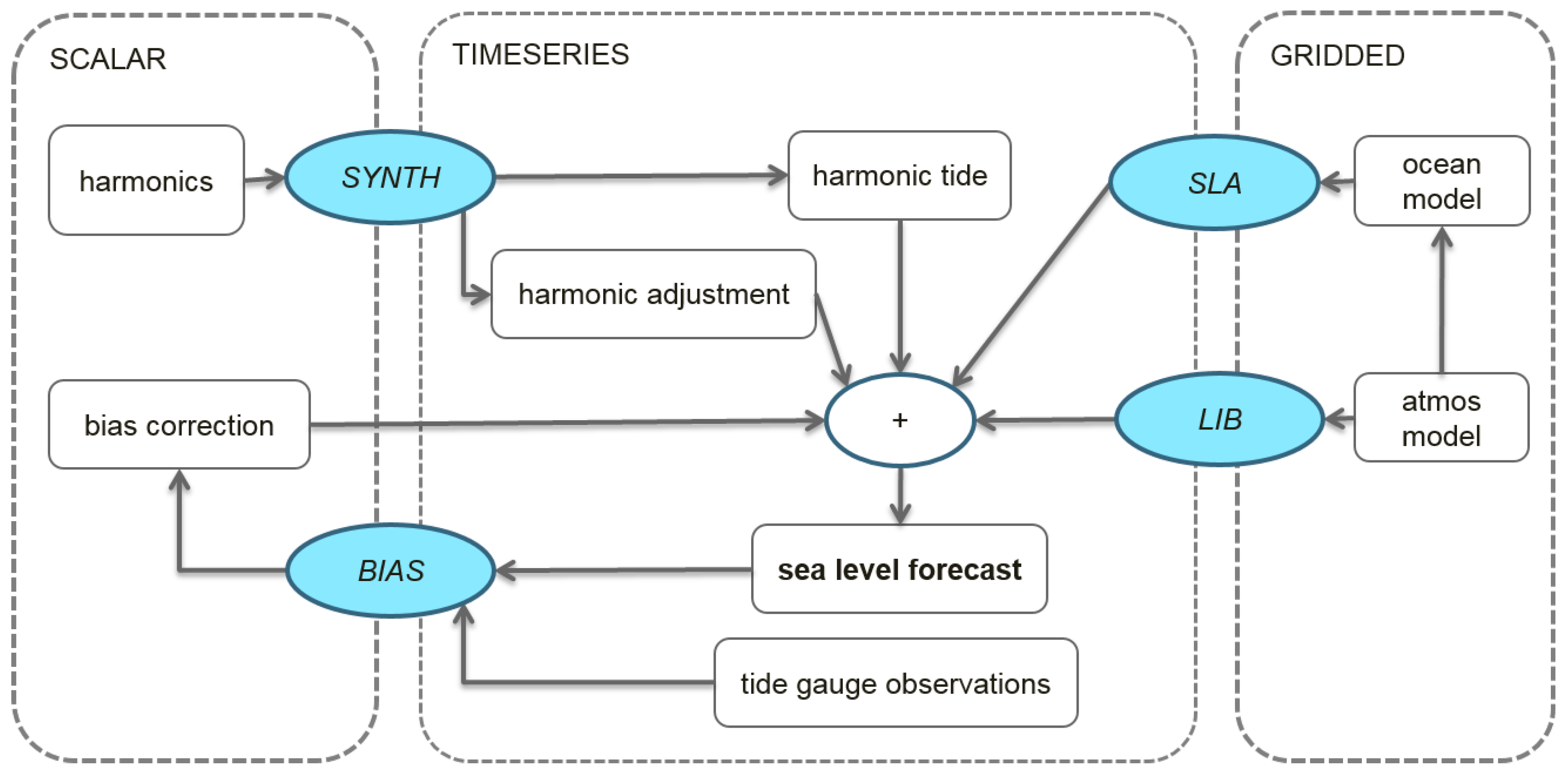
2.2. Superposition
2.3. Input: Data Assimilating Primitive Equation Forecasts
2.4. Input: Tidal Harmonics
- full set of tidal harmonics: typically 114 constituents.
- subset assigned apriori to be primarily non-gravitational in expression: Sa, SSa, Mm, Msf and S1.
2.5. Input: Bias Correction
3. Evaluation
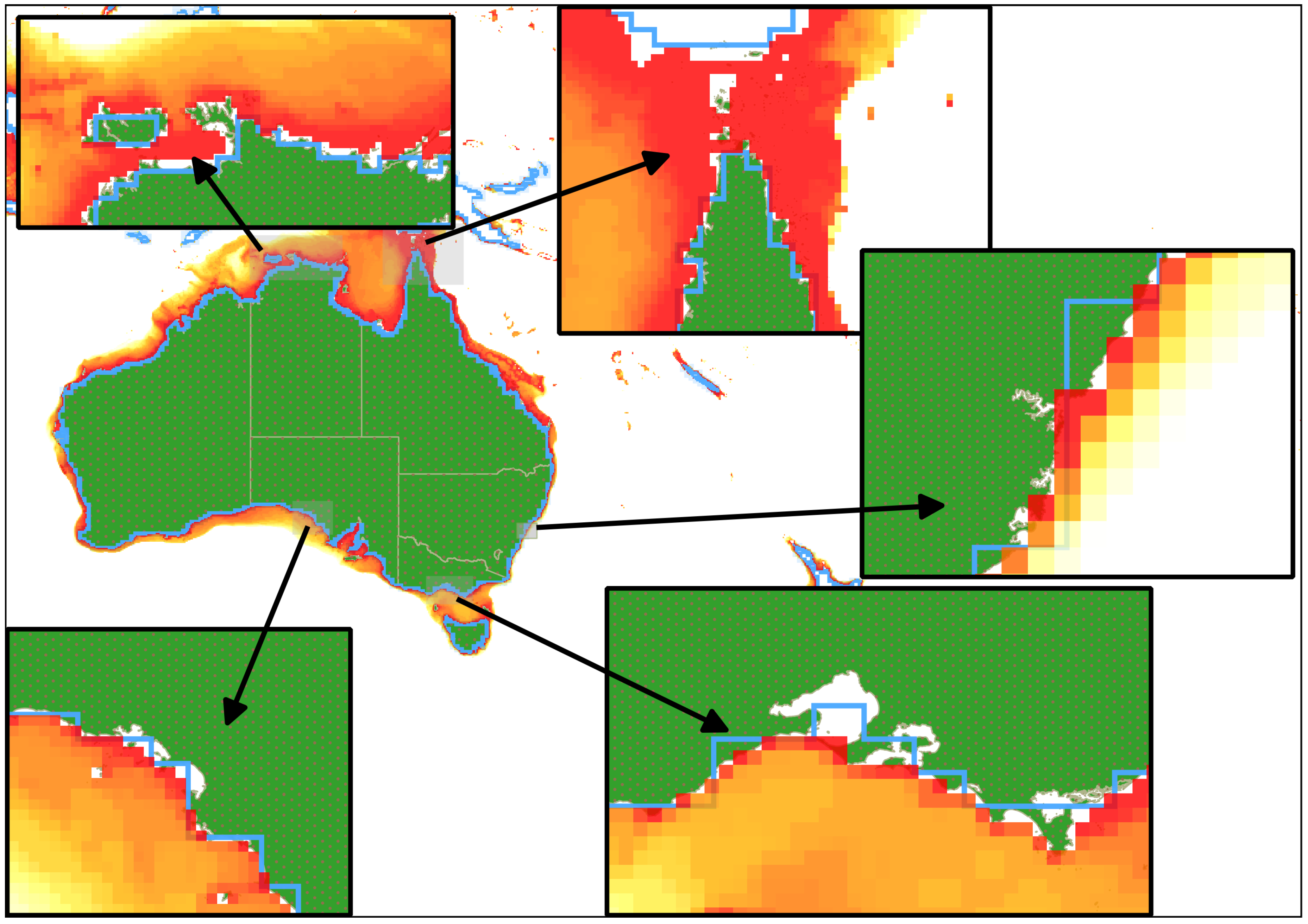
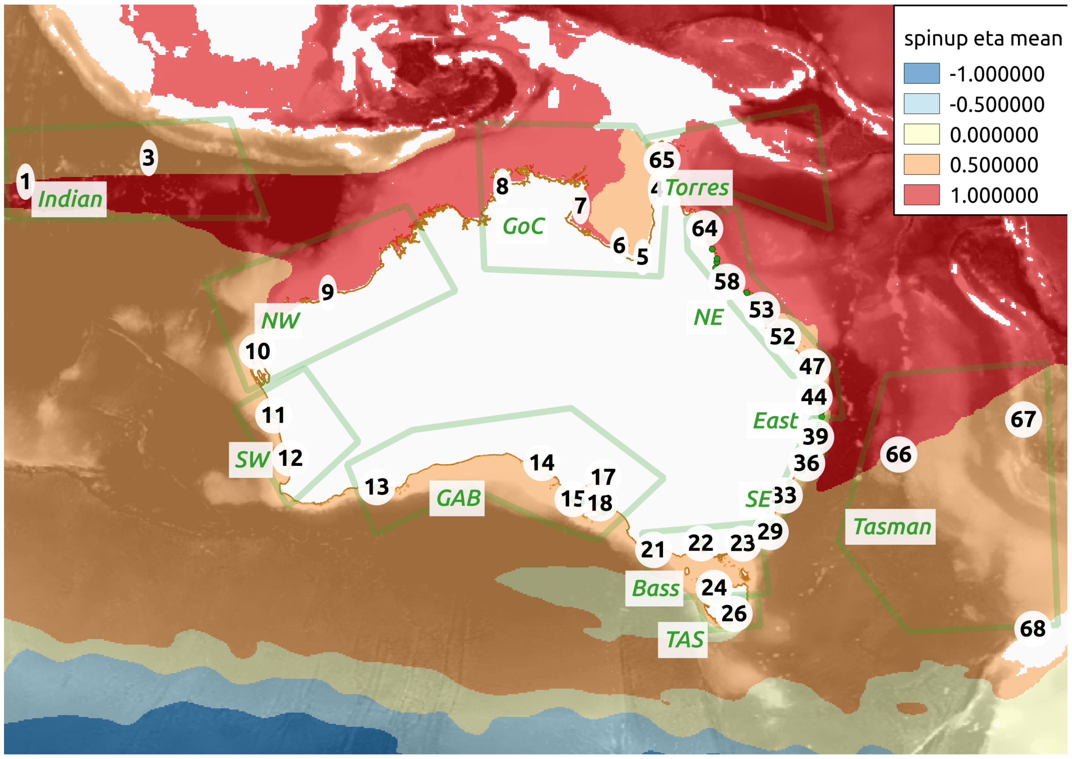
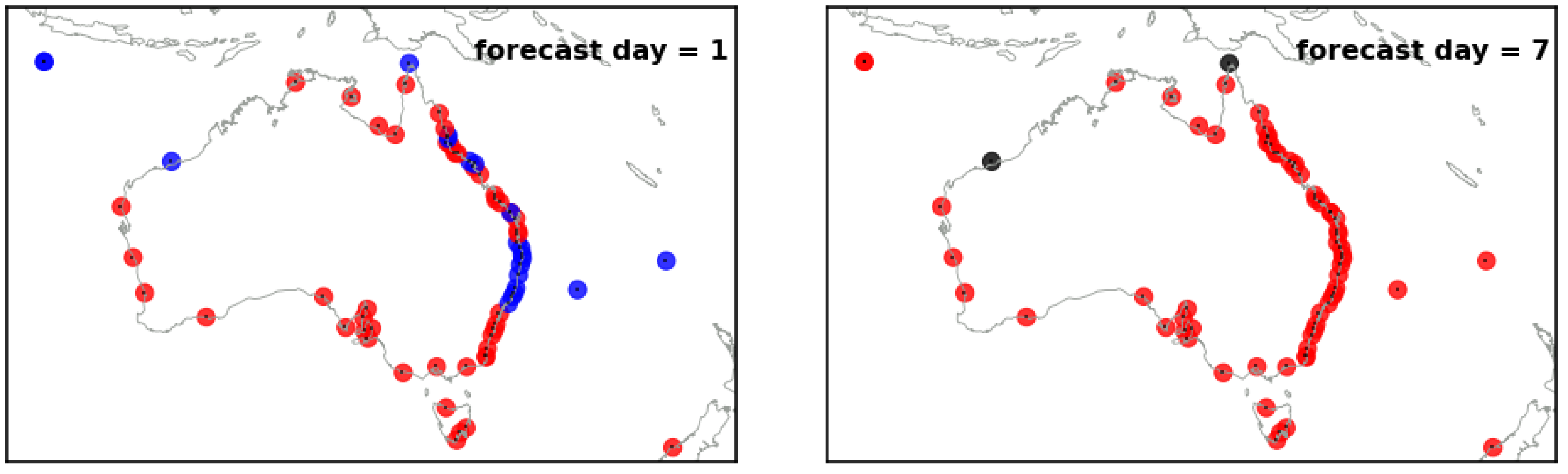
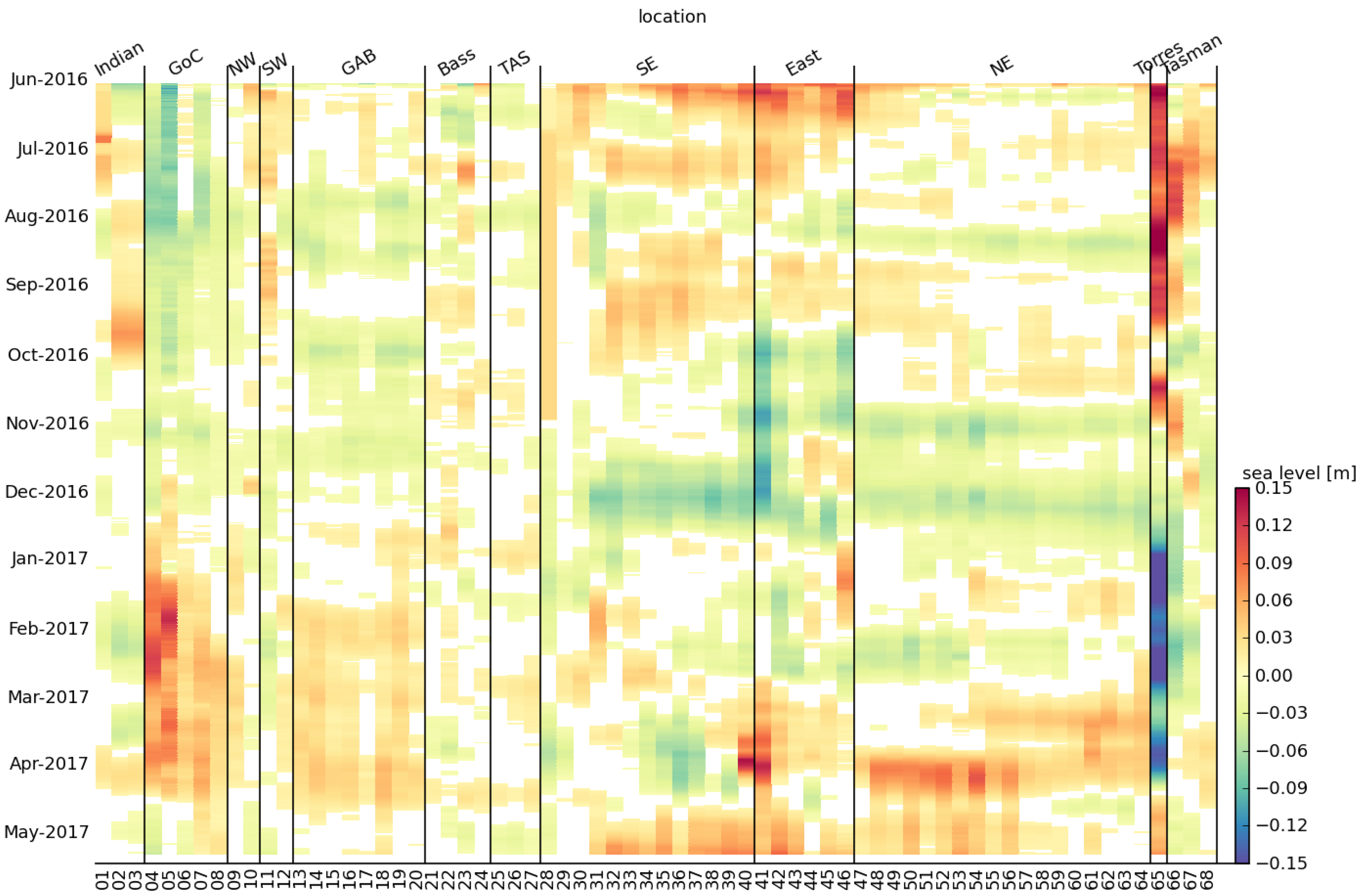
3.1. Geographic Overview
3.2. Forecast Goodness as Routine Guidance
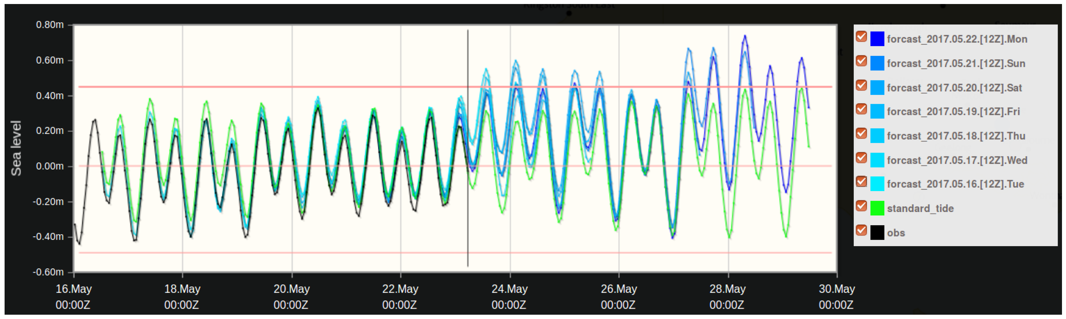
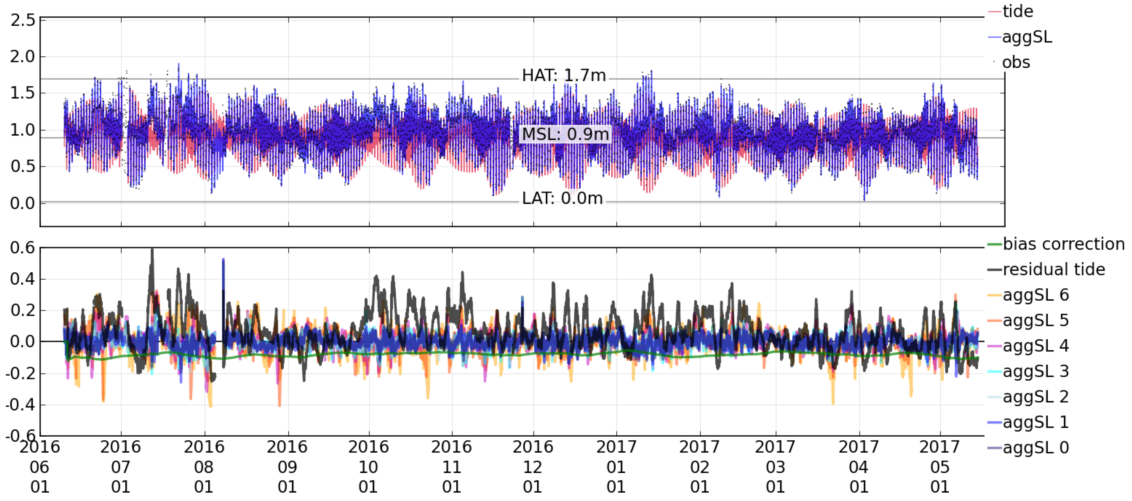
3.3. Highlighted Behaviour
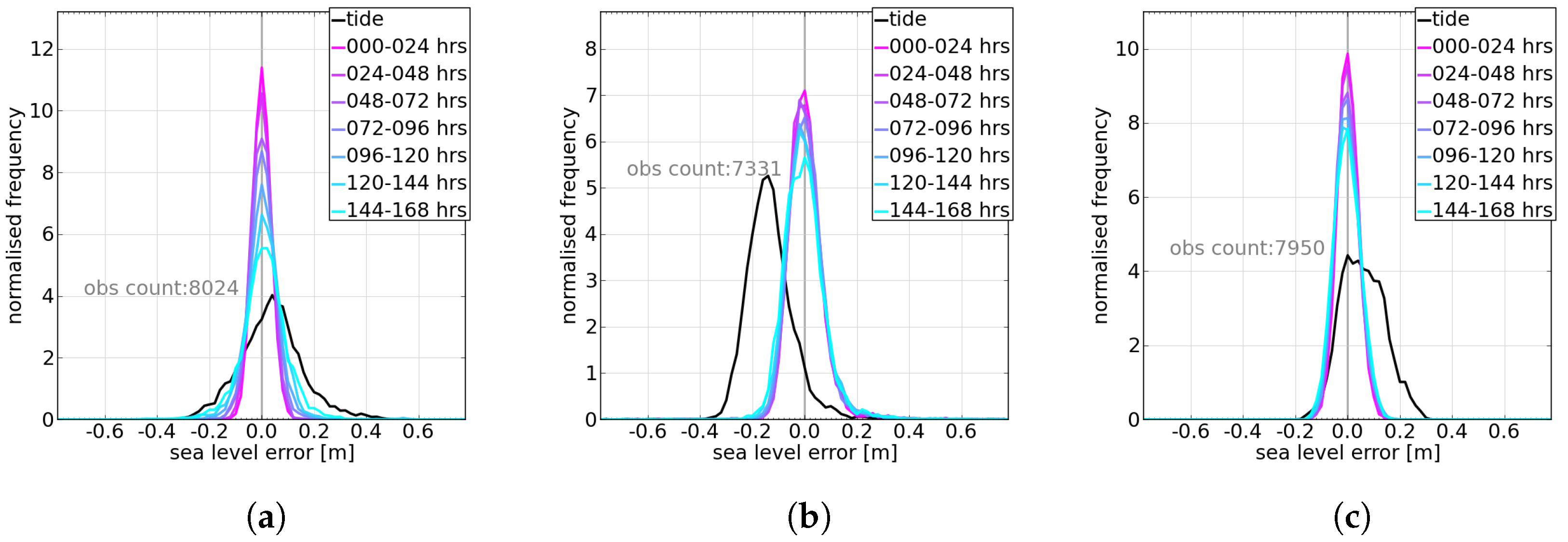
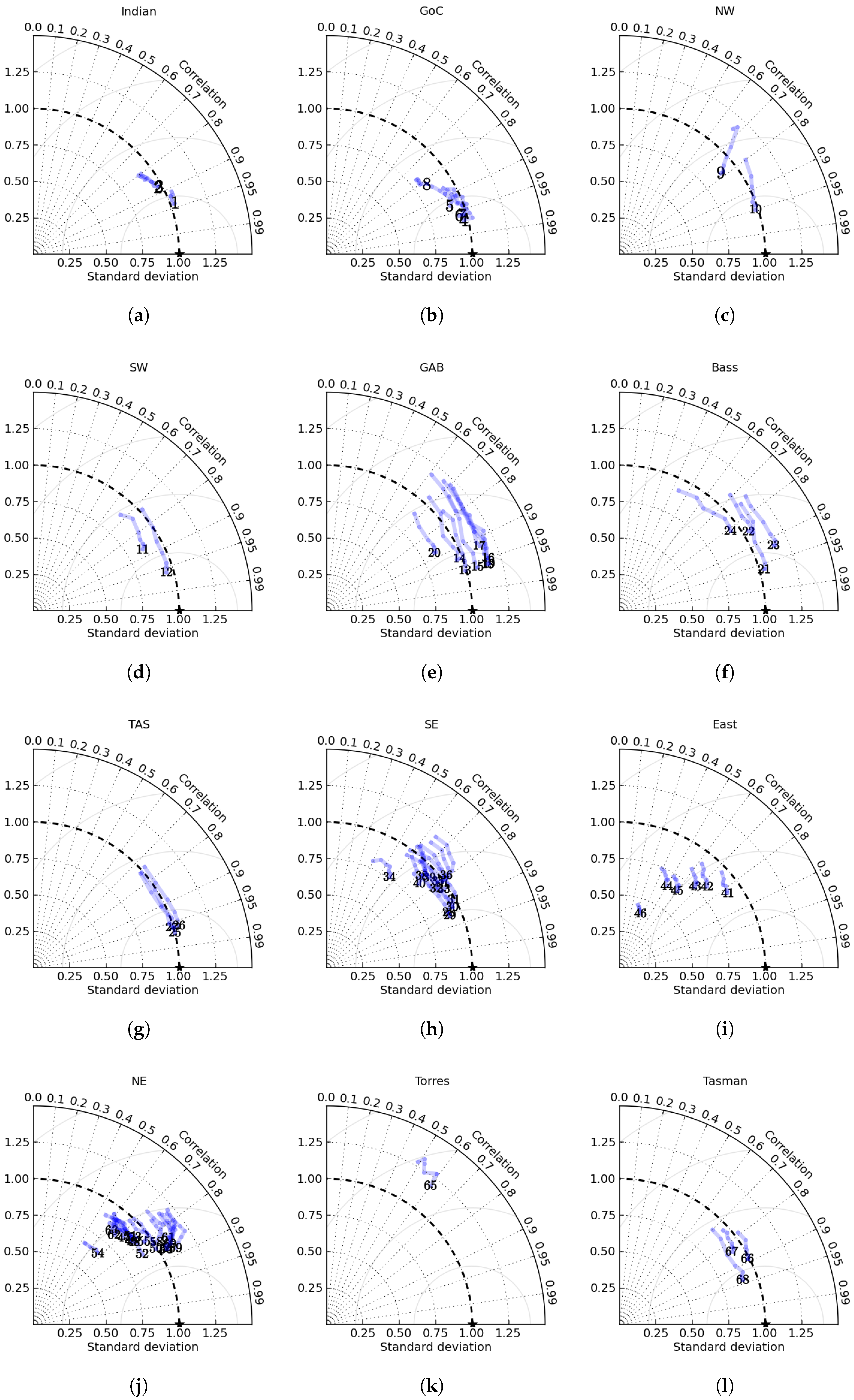
3.4. Skill Summary: Non-Tidal Information Decay
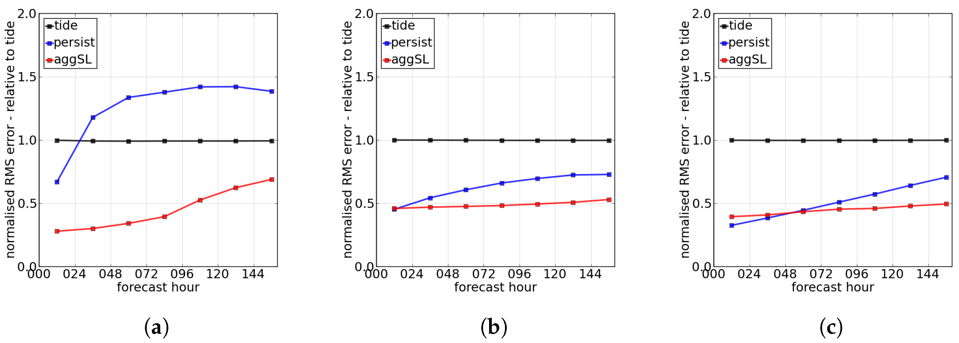
3.5. Skill Summary: Comparison Against ‘Tide + Persisted Residual’
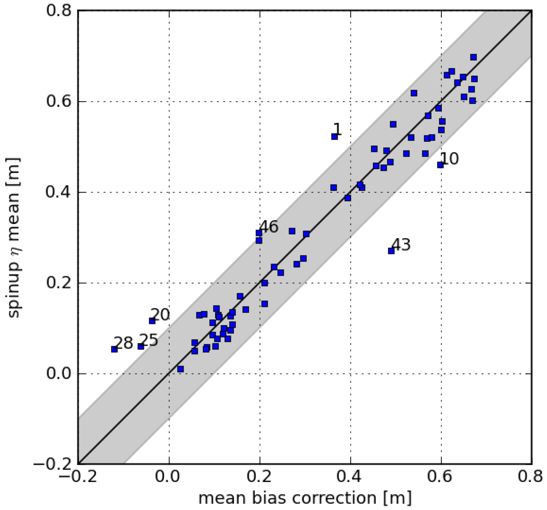
4. Role of Bias Correction Component
5. Discussion
5.1. Adequacy and Value
5.2. Spatial Interpolation
5.3. Extensions
Acknowledgments
Author Contributions
Conflicts of Interest
Abbreviations
| aggSL | Aggregate Sea Level |
| AHD | Australian Height Datum |
| ATGF | Astronomical Tide Producing Forces |
| BoM | Australian Bureau of Meteorology |
| HAT | Highest Astronomical Tide—conventional tidal plane |
| LAT | Lowest Astronomical Tide—conventional tidal plane |
| LIB | Local Inverse Barometer Approximation |
| MDT | Mean Dynamic Topography |
| MSL | Mean Sea Level—conventional tidal plane |
| MOM | Modular Ocean Model |
| NWP | Numerical Weather Prediction |
| OceanMAPS | Ocean Model, Analysis and Prediction System |
| RMSE | Root Mean Square Error |
| SLA | Sea Level Anomaly |
References
- Bell, M.J.; Lefèbvre, M.; Le Traon, P.Y.; Smith, N.; Wilmer-Becker, K. GODAE The Global Ocean Data Assimilation Experiment. Oceanography 2009, 22, 14–21. [Google Scholar] [CrossRef]
- Pugh, D.; Woodworth, P. Sea-Level Science: Understanding Tides, Surges, Tsunamis and Mean Sea-Level Changes; Cambridge University Press: Cambridge, UK, 2014. [Google Scholar]
- Box, G. Robustness in the strategy of scientific model building. Robust. Stat. 1979. [Google Scholar] [CrossRef]
- Melet, A.; Almar, R.; Meyssignac, B. What dominates sea level at the coast: A case study for the Gulf of Guinea. Ocean Dyn. 2016, 66, 623–636. [Google Scholar] [CrossRef]
- Haigh, I.D.; Wijeratne, E.M.S.; MacPherson, L.R.; Pattiaratchi, C.B.; Mason, M.S.; Crompton, R.P.; George, S. Estimating present day extreme water level exceedance probabilities around the coastline of Australia: Tides, extra-tropical storm surges and mean sea level. Clim. Dyn. 2013, 42, 121–138. [Google Scholar] [CrossRef]
- Haigh, I.D.; MacPherson, L.R.; Mason, M.S.; Wijeratne, E.M.S.; Pattiaratchi, C.B.; Crompton, R.P.; George, S. Estimating present day extreme water level exceedance probabilities around the coastline of Australia: Tropical cyclone-induced storm surges. Clim. Dyn. 2013, 42, 139–157. [Google Scholar] [CrossRef]
- Woodham, R.; Brassington, G.B.; Robertson, R.; Alves, O. Propagation characteristics of coastally trapped waves on the Australian Continental Shelf. J. Geophys. Res. Oceans 2013, 118, 4461–4473. [Google Scholar] [CrossRef]
- Ridgway, K.R. The 5500-km-long boundary flow off western and southern Australia. J. Geophys. Res. 2004. [Google Scholar] [CrossRef]
- Church, J.A.; Freeland, H. Coastal-trapped waves on the east Australian continental shelf. I: Propagation of modes. J. Phys. Oceanogr. 1986, 16, 1929–1943. [Google Scholar] [CrossRef]
- Allen, S.C.R.; Greenslade, D.J.M. A Spectral Climatology of Australian and South-West Pacific Tide Gauges; CAWCR Technical Reports; Centre for Australian Weather and Climate Research: Melbourne, VIC, Australia, 2009.
- Cartwright, D.E. Tides; Cambridge University Press: Cambridge, UK, 2000. [Google Scholar]
- Petersen, A. Simulating Nature; Chapman and Hall/CRC: London, UK, 2012. [Google Scholar]
- Schiller, A.; Brassington, G.B. Operational Oceanography in the 21st Century; Springer Science + Business Media: Berlin, Germany, 2011. [Google Scholar]
- Harper, K.C. Weather by the Numbers; The MIT Press: Cambridge, MA, USA, 2008. [Google Scholar]
- Paramygin, V.; Sheng, Y.; Davis, J. Towards the Development of an Operational Forecast System for the Florida Coast. J. Mar. Sci. Eng. 2017, 5, 8. [Google Scholar] [CrossRef]
- Yang, Z.; Richardson, P.; Chen, Y.; Kelley, J.; Myers, E.; Aikman, F.; Peng, M.; Zhang, A. Model Development and Hindcast Simulations of NOAA’s Gulf of Maine Operational Forecast System. J. Mar. Sci. Eng. 2016, 4, 77. [Google Scholar] [CrossRef]
- Wei, E.; Zhang, A.; Yang, Z.; Chen, Y.; Kelley, J.; Aikman, F.; Cao, D. NOAA’s Nested Northern Gulf of Mexico Operational Forecast Systems Development. J. Mar. Sci. Eng. 2014, 2, 1–17. [Google Scholar] [CrossRef]
- Peng, M.; Schmalz, R.A., Jr.; Zhang, A.; Aikman, F., III. Towards the Development of the National Ocean Service San Francisco Bay Operational Forecast System. J. Mar. Sci. Eng. 2014, 2, 247–286. [Google Scholar] [CrossRef]
- Hendershott, M. Long waves and ocean tides. In Evolution of Physical Oceanography; The MIT Press: Cambridge, MA, USA, 1981. [Google Scholar]
- Foreman, M.G.G.; Cherniawsky, J.Y.; Ballantyne, V. Versatile Harmonic Tidal Analysis: Improvements and Applications. J. Atmos. Ocean. Technol. 2009. [Google Scholar] [CrossRef]
- Groves, G.W.; Reynolds, R.W. An Orthogonalized Convolution Method of Tide Prediction. J. Geophys. Res. 1975, 80, 4131–4138. [Google Scholar] [CrossRef]
- Leffler, K.; Jay, D. Enhancing tidal harmonic analysis: Robust (hybrid L1/L2L1/L2) solutions. Cont. Shelf Res. 2009, 29, 78–88. [Google Scholar] [CrossRef]
- Smith, A.; Ambrosius, B.; Wakker, K.F.; Woodworth, P.L.; Vassie, J.M. Comparison between the harmonic and response methods of tidal analysis using TOPEX/POSEIDON altimetry. J. Geod. 1997, 71, 695–703. [Google Scholar] [CrossRef]
- Mapping, I.C.o.S. Australian Tides Manual; Technical Report; Permanent Committee on Tides and Mean Sea Level: Wollongong, Australia, 2014.
- Parker, B.B. Tidal Analysis and Prediction; Technical Report; National Oceanic and Atmospheric Administration—Center for Operational Oceanographic Products and Services: Silver Spring, MD, USA, 2007.
- Ray, R.; Egbert, G.D. The Global S1 Tide. J. Phys. Oceanogr. 2004, 34, 1922. [Google Scholar] [CrossRef]
- Horsburgh, K.J.; Williams, J.A.; Flowerdew, J.; Mylne, K. Aspects of operational forecast model skill during an extreme storm surge event. J. Flood Risk Manag. 2008, 1, 213–221. [Google Scholar] [CrossRef]
- Egbert, G.D.; Bennett, A.F. Data assimilation methods for ocean tides. Elsevier Oceanogr. Ser. 1996. [Google Scholar] [CrossRef]
- Greenslade, D.J.M.; Warne, J.O. Assessment of the Effectiveness of a Sea-Level Observing Network for Tsunami Warning. J. Waterw. Port Coast. Ocean Eng. 2012, 138, 246–255. [Google Scholar] [CrossRef]
- Horsburgh, K.; De Vries, H. Guide to Storm Surge Forecasting; Technical Report; World Meteorological Organization: Geneva, Switzerland, 2011. [Google Scholar]
- Mourre, B.; Crosnier, L.; Provost, C.L. Real-time sea-level gauge observations and operational oceanography. Philos. Trans. R. Soc. A 2006, 364, 867–884. [Google Scholar] [CrossRef] [PubMed]
- Taylor, A.J.; Brassington, G.B.; Nader, J. Assessment of BLUElink OceanMAPSv1.0b Against Coastal Tide Gauges; Technical Report; Centre for Australian Weather and Climate Research: Melbourne, VIC, Australia, 2010.
- Tilburg, C.E.; Garvine, R.W. A Simple Model for Coastal Sea Level Prediction. Weather Forecast. 2004. [Google Scholar] [CrossRef]
- Taylor, A.J.; Smith, A.; Wang, W.; Robinson, J.; Brassington, G.B. Ocean meets river: Connecting Bureau of Meteorology ocean forecasts and river height predictions for improved flood warnings. In Proceedings of the 19th International Congress on Modelling and Simulation, Perth, Australia, 12–16 December 2011. [Google Scholar]
- Brassington, G.B.; Pugh, T.; Spillman, C.; Schulz, E.; Beggs, H.; Schiller, A.; Oke, P.R. BLUElink> Development of Operational Oceanography and Servicing in Australia. J. Res. Pract. Inf. Technol. 2007, 39, 151–164. [Google Scholar]
- Bureau of Meterology. Implementation of OceanMAPS (BLUElink> Ocean Forecast System); Technical Report; Bureau of Meteorology: Melbourne, VIC, Australia, 2007.
- Bureau of Meterology. Operational Upgrades to OceanMAPS (BLUElink> Ocean Forecast System); Technical Report; Bureau of Meteorology: Melbourne, VIC, Australia, 2011.
- Brassington, G.B.; Freeman, J.; Huang, X.; Pugh, T.; Oke, P.; Sandery, P.A.; Taylor, A.J.; Andreu-Burillo, I.; Schiller, A.; Griffin, D.; et al. Ocean Model, Analysis and Prediction System: Version 2; Technical Report; Centre for Australian Weather and Climate Research: Melbourne, VIC, Australia, 2012.
- Griffies, S.M.; Harrison, M.; Pacanowski, R. A Technical Guide to MOM4; Technical Report; NOAA/Geophysical Fluid Dynamics Laboratory: Princeton, NJ, USA, 2008.
- Oke, P.; Brassington, G.B.; Griffin, D. The Bluelink ocean data assimilation system (BODAS). Ocean Model. 2008, 21, 46–70. [Google Scholar] [CrossRef]
- Bureau of Meterology. APS2 Upgrade to the ACCESS-G Numerical Weather Prediction System; Technical Report; Bureau of Meteorology: Melbourne, VIC, Australia, 2016.
- Brassington, G.B. Multicycle ensemble forecasting of sea surface temperature. Geophys. Res. Lett. 2013, 40, 6191–6195. [Google Scholar] [CrossRef]
- Mathers, E.L.; Woodworth, P.L. A study of departures from the inverse-barometer response of sea level to air-pressure forcing at a period of 5 days. Q. J. R. Meteorol. Soc. 2004, 130, 725–738. [Google Scholar] [CrossRef]
- Murphy, A.H. What Is a Good Forecast? An Essay on the Nature of Goodness in Weather Forecasting. Weather Forecast. 1993, 8, 281–293. [Google Scholar] [CrossRef]
- Taylor, K. Summarizing Multiple Aspects of Model Performance in a Single Diagram; Technical Report; Program For Climate Model Diagnosis And Intercomparison University Of California, Lawrence Livermore National Laboratory: Livermore, CA, USA, 2000.
- Slobbe, D.C.; Verlaan, M.; Klees, R.; Gerritsen, H. Obtaining instantaneous water levels relative to a geoid with a 2D storm surge model. Cont. Shelf Res. 2013, 52, 172–189. [Google Scholar] [CrossRef]
- Oke, P.; Griffin, D.; Schiller, A. Evaluation of a near-global eddy-resolving ocean model. Geosci. Model Dev. 2013, 6, 591–615. [Google Scholar] [CrossRef]


© 2017 by the authors. Licensee MDPI, Basel, Switzerland. This article is an open access article distributed under the terms and conditions of the Creative Commons Attribution (CC BY) license (http://creativecommons.org/licenses/by/4.0/).
Share and Cite
Taylor, A.; Brassington, G.B. Sea Level Forecasts Aggregated from Established Operational Systems. J. Mar. Sci. Eng. 2017, 5, 33. https://doi.org/10.3390/jmse5030033
Taylor A, Brassington GB. Sea Level Forecasts Aggregated from Established Operational Systems. Journal of Marine Science and Engineering. 2017; 5(3):33. https://doi.org/10.3390/jmse5030033
Chicago/Turabian StyleTaylor, Andy, and Gary B. Brassington. 2017. "Sea Level Forecasts Aggregated from Established Operational Systems" Journal of Marine Science and Engineering 5, no. 3: 33. https://doi.org/10.3390/jmse5030033
APA StyleTaylor, A., & Brassington, G. B. (2017). Sea Level Forecasts Aggregated from Established Operational Systems. Journal of Marine Science and Engineering, 5(3), 33. https://doi.org/10.3390/jmse5030033