1. Introduction
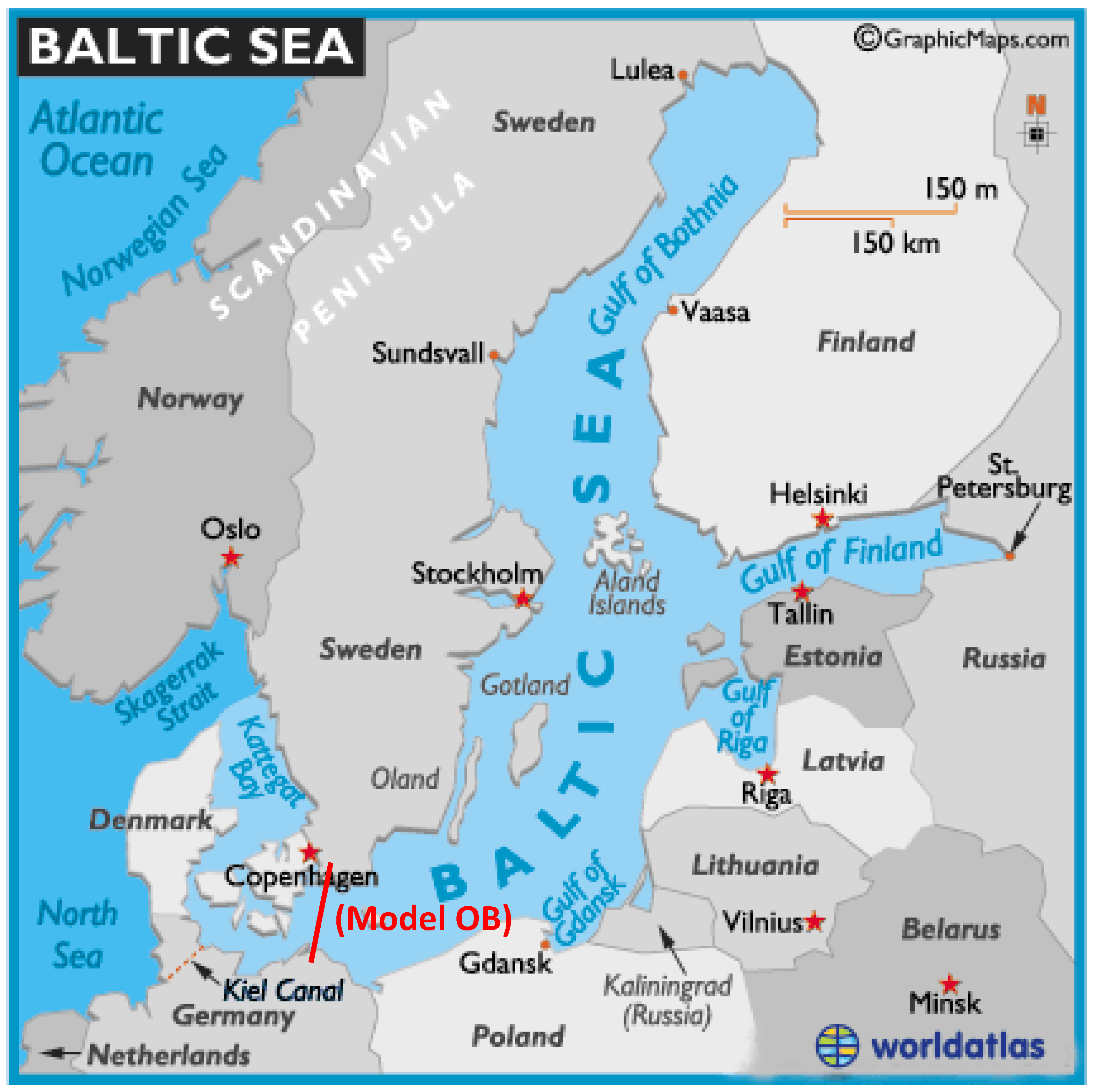
The Baltic Sea is a brackish sea located in northern Europe from 53° N to 66° N latitude and from 20° E to 26° E longitude. It is connected to the Atlantic Ocean via the Danish Straits. The Baltic Ice Lake was born 13,000 years ago and its present brackish state emerged 7000 years ago. For 2000 years, the salinity has been close to the present level (mean salinity: 7 parts per thousand). The Baltic Sea borders nine coastal countries with a total population of 85 million people (see
Figure 1, [
1]). The maximum length and width are 1600 km and 193 km, respectively. The surface area is 377,000 km
2, with an average depth of 55 m and a water volume of 20,000 km
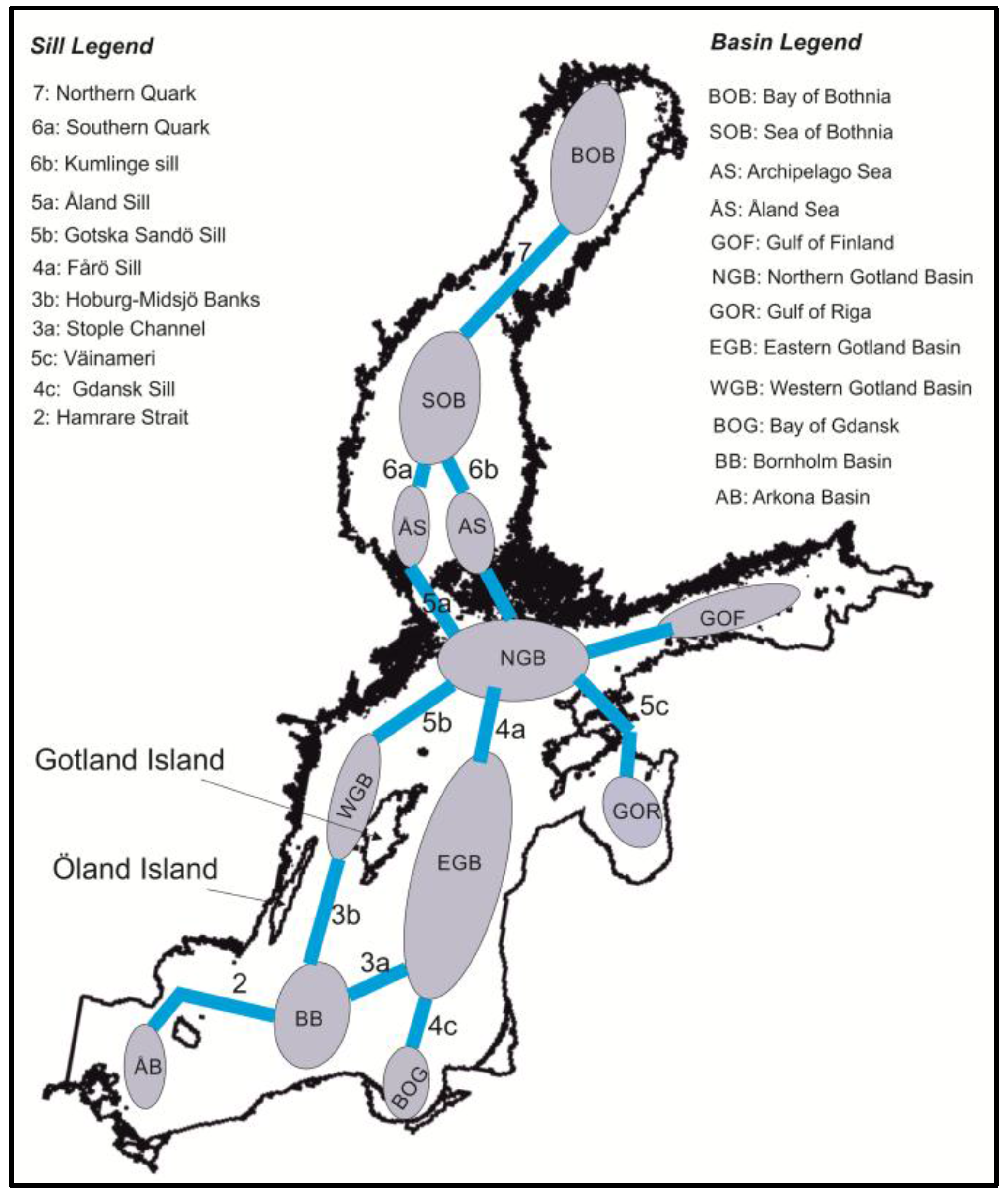
3. Its maximum depth is 459 m, which is located between Stockholm and the Island of Gotland. The Baltic Sea is a shallow sea that consists of a series of basins interconnected through narrow sills (
Figure 2).
In spite of the Baltic Sea HELCOM agreement signed in 1974, the state of the Baltic Sea has worsened (
http://www.helcom.fi). Nutrient levels in the water and sediments are high, and poor oxygen conditions and “dead bottoms” exist in large archipelago areas of both Sweden and Finland [
2]. However, during the past few decades there have been considerable efforts towards better and more sustainable management of the Baltic Sea. Here, the hydrodynamics of the Baltic Sea, which has been the subject of intensive research since the 1930s, plays a major role. The number of available journal articles and other publications exceeds several hundred. The foci of these studies are exchange processes, especially salt transport from the North Sea, and water age. Some of the main contributors are Meier [
3], and Lehman and Hinrichsen [
4]. Here, the work of Omstedt et al. [
5] should be mentioned as it presents the state of knowledge on various hydrodynamic features of the Baltic Sea. There are also several excellent books covering many different aspects, including Feistel et al. [
6], Leppäranta and Myrberg [
7], and Harff et al. [
8]. For a general literature review, the interested reader is referred to the comprehensive review given by Dargahi and Cvetkovic [
9].
The present study concerns the hydrodynamics of the Baltic, with a focus on the details of stratification, which is the primary feature of the sea. The novel features of the work are the relatively long simulation period of 10 years and the use of a complete set of external boundary conditions with maximum spatial and temporal resolution, in combination with highly accurate bathymetry. The main objectives were to create an accurate and validated 3D hydrodynamic model for investigating specific stratification characteristics that have not been addressed in the previous studies. In the following paragraph we present a short summary of previous research works on stratification.
The Baltic Sea is highly stratified by strong vertical salinity and temperature gradients. The stratification is commonly referred to as a two-layer structure that consists of an upper and a lower layer. A transitional middle layer exists between the upper and lower layers, which are known as halocline and thermocline, respectively. There is a significant variation in the depth of the halocline, from 40 m to 80 m in deeper regions to 10 m–30 m in shallower regions [
7]. The lower values are found in the Gulf of Riga (mean value = 25 m), and Arkona Basin, with a mean value of 25 m for both regions [
10,
11]. The surface salinity varies in the north with a mean value of 3 ppt (parts per thousand) to 8 ppt to the south, i.e., the Arkona Basin. The corresponding mean value at the lower layer is in the range of 4–12.5 ppt. However, the salinities are considerably higher in the open sea. The mean values in the Kattegatt (the region in which the Baltic Sea drains through the Danish strait) are 22 ppt and 31 ppt, respectively (same references). Suominen et al. [
12] studied surface salinity gradients and their temporal fluctuations in the Archipelago Sea of the northern Baltic Sea based on field salinity data for the time period July 2007–August 2008. They identified a broad scale gradient from low salinity in the shallow inner bays to the high salinity in the open sea areas towards the Baltic proper. The steepest gradients were observed in the semi-closed part of the archipelago. One important result was that the use of temporal mean values of salinity was insufficient for coastal management purposes in the region.
The halocline depth is controlled by wind-induced mixing and advection, which appears to change little over time. Väli et al. [
11] looked into variations of the halocline during 1961–2007. Two periods were identified with shallow halocline during 1970–1975, and with deep halocline during 1990–1995. The main conclusion was that the freshwater content and absolute wind speed control the halocline depth in the Baltic Sea. However, they found the wind speed to have a moderate impact on the mean halocline depth in the Baltic proper due to the low impact of runoff.
An important issue is the effect of fresh water on stratification in the Baltic Sea. Hordoir and Meier [
13] studied the dynamics of fresh water, which is released during spring into the Baltic proper. They showed that the fresh water only reaches the center of the Baltic proper after late summer. A small amount of fresh water may reach the entrance of the Baltic Sea during one season. The arrival of fresh water increases vertical stratification, which can in turn trigger the onset of the spring blooms. They also found that the seasonal changes in the fresh water outflow were closely connected with those of the zonal wind. An important result was the correlation of the annual variability of the seasonal freshwater outflow maximum with the North Atlantic Oscillation.
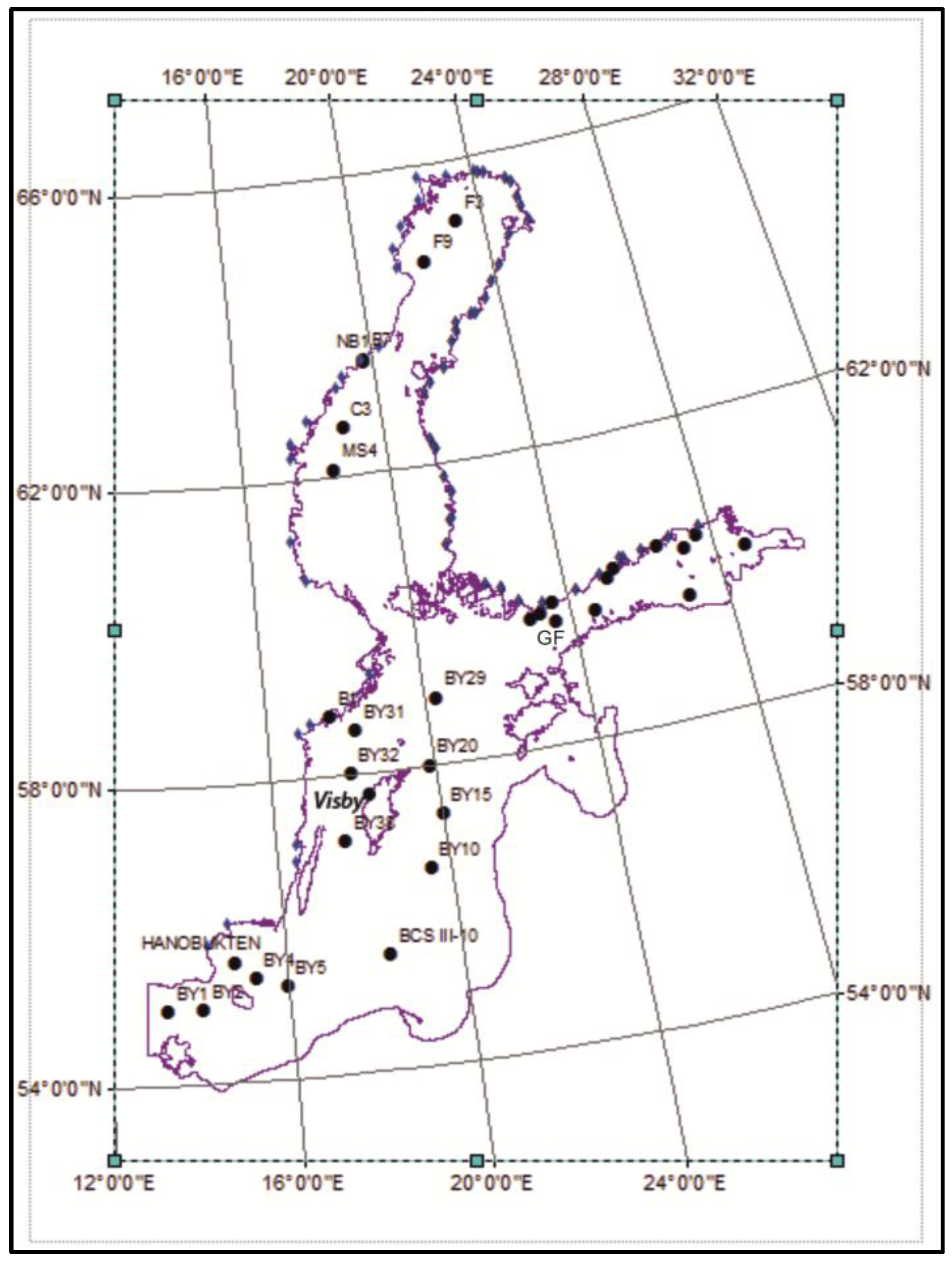
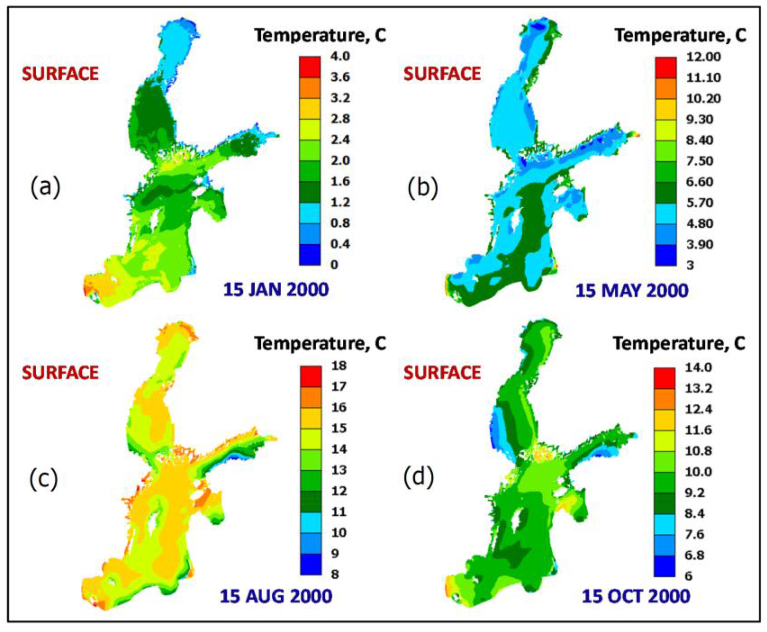
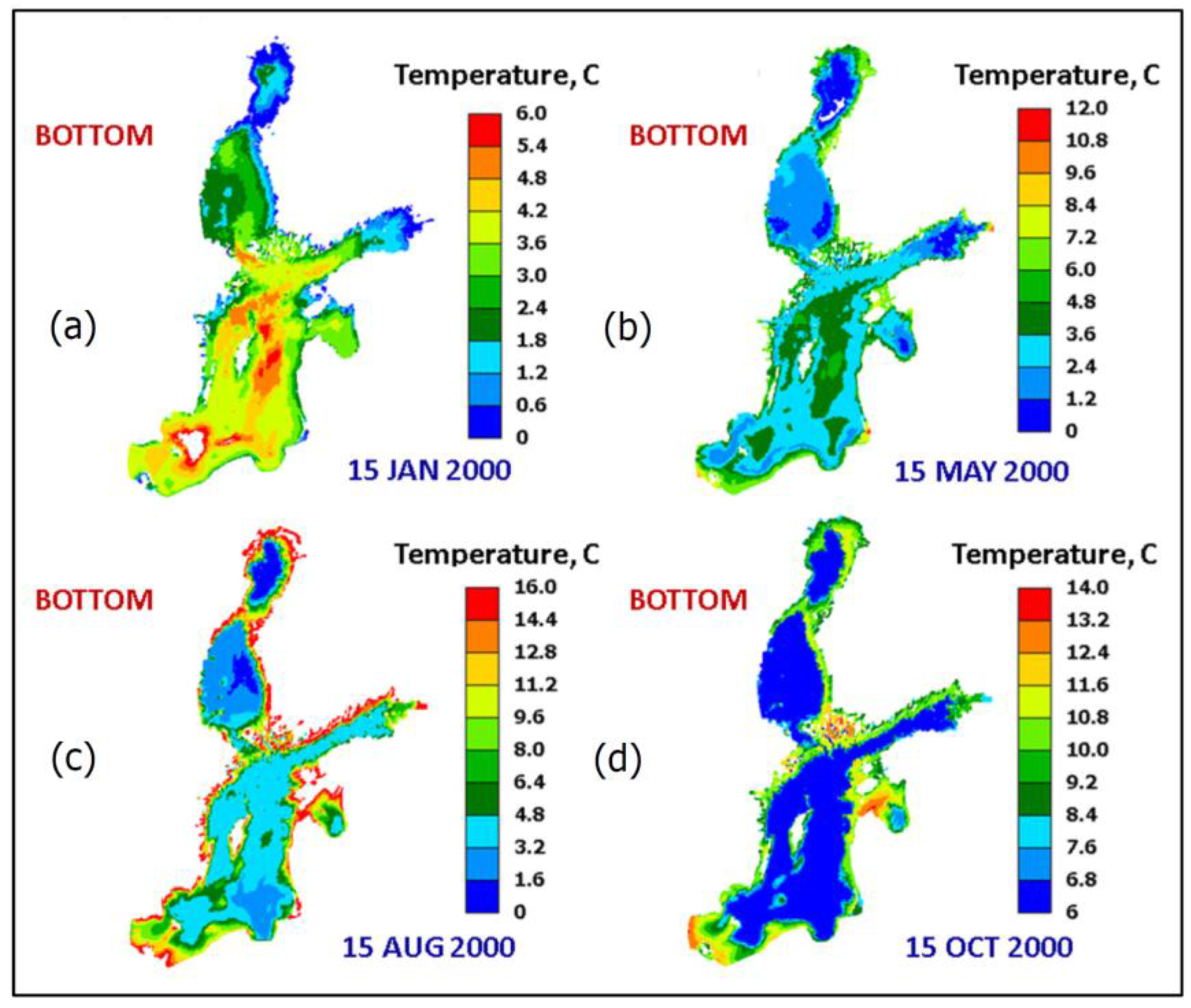
The temperature stratification in the Baltic Sea has a mean three-layer structure in analogy to the salinity stratification. The layers are commonly referred to as the epilimnion (upper layer), thermocline (middle layer), and hypolimnion (lower layer). In similarity with the other large water bodies, there is a seasonal stratification cycle, which is driven by the variations in the energy balance. However, in the case of the Baltic Sea there are two specific features. First, fall and spring overturns are not well defined, and second, the hypolimnion has a nearly constant temperature, with few seasonal variations. During the winter periods, the epilimnion layer has a lower temperature than the hypolimnion layer. The Baltic Sea is monitored using 22 stations, as shown in
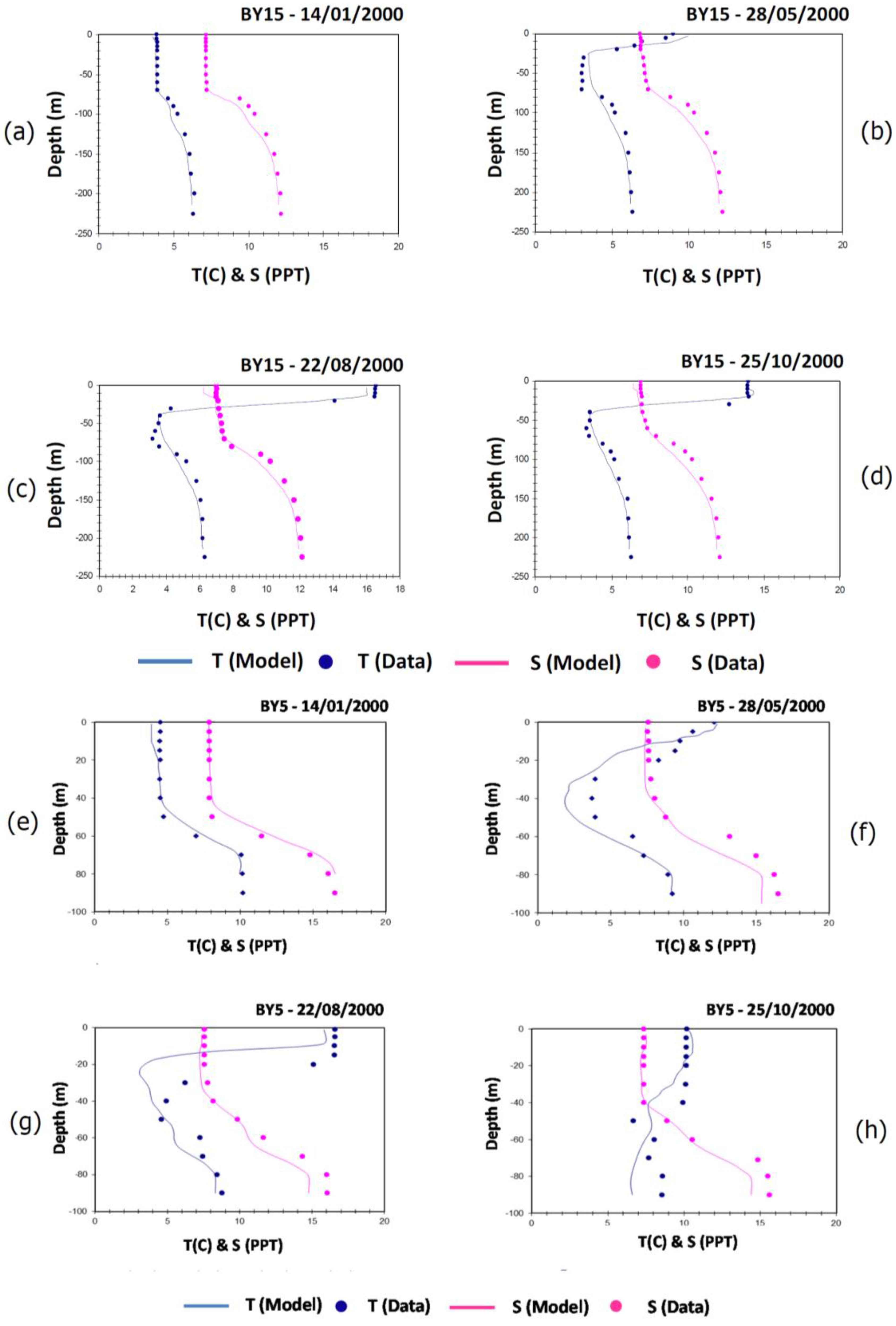
Figure 3. A typical temperature difference at the gauge station BY15 is about 5 °C. In the spring, following the ice melt, a thin warmer surface layer rapidly develops and sets up the thermocline. The thickness of the layer varies considerably from north to south, but a mean value of about 15 m can be used. The temperature gradient is high within the epilimnion layer. For instance, at BY15, the temperature can vary from 1.5 °C to 5 °C within a depth of 60 m. Below this depth, the temperatures increase rapidly to reach the constant temperature of the hypolimnion layer (about 5 °C). The layer with transitional temperature is known as the dicothermal layer, which is a cold layer sandwiched between two layers with higher temperatures (dicothermal). The dicothermal layer was first discovered by the Ekman expedition of 1877 to the Baltic Sea (see Fonselius [
14]). The layer appears to originate from the vertical convection of the surface water in the winter. It is further explained that this cold surface water from the previous winter was preserved between the thermocline and halocline (see Fonselius [
14]). The dicothermal layer develops at high latitudes with cold climates. Peter [
15] reports the development of a layer with a thickness of 100 m in the Indian Ocean region of the Antarctic. The reported thickness in the Baltic Sea is in the range of 5–30 m, which persists during the summer and disappears during the autumn [
7]. Here, we note that the measured temperature profiles in the southern basins confirm the formation of the dicothermal layer even during the spring.
The stratification is strongest during the summer due to high solar radiation input and warm air temperatures. The surface layer thickness increases to about 20 m during the summer period due to wind induced vertical mixing The temperature within the layer is nearly constant. Below the surface layer, a strong thermocline develops that has a sharp temperature drop of about 10 °C over a depth of about 10 m (e.g., temperature profile at BY15). There is also a dicothermal layer below the thermocline, which has a thickness of about 30 m at BY15. The hypolimnion layer has a relatively constant temperature of 4–5 °C, which is close to the temperature of maximum density of water. The layer thickness varies considerably, from about 30 m in shallow regions to 100 m in the deeper region. The negative effect of the strong stratification limits the exchange between the epilimnion and hypolimnion layers.
During autumn, the surface heat losses start to increase and the thermocline depth deepens. For instance, in the Eastern Gotland Basin, the thermocline reaches a depth of about 40 m. The lower temperatures cause the temperature gradient to decrease, which in turn weakens the thermocline. The temperature changes in the thermocline cause a weak positive temperature gradient to develop in the hypolimnion layer (e.g., 1 °C over 100 m).
2. Materials and Methods
The materials used to model the Baltic Sea consisted of basic geometrical and various flow and meteorological data for the period 2000–2009 as listed below.
The shoreline and the bathymetry in GIS format.
Daily flow discharges for 24 Swedish rivers, 38 Finnish rivers, and five Eastern European rivers (i.e., the Daugava, Neman, Neva, Odra, and Vistula).
Monthly mean flow discharge for four Eastern European rivers (i.e., Lielupe, Narva, Pärnu, and Narva). The daily records were not available.
Water temperature for all the rivers.
The forcing meteorological data (air temperature, dew point, cloud cover, pressure, wind speed, and wind direction) at 3-h intervals as grid data.
Precipitation as rain intensity at 19 stations at daily intervals.
Water quality data at 15-day intervals for 22 different stations spread across the sea. The data included water temperature, salinity, dissolved oxygen, and phosphorous.
Wave heights and sea and water levels at several stations across the sea.
The main data sources were the Swedish Meteorological and Hydrological Institute, SMHI [
16], and the Finnish Meteorological Institute, FMI [
17]. The gridded meteorological data were obtained from
http://www.smhi.se/en/research/research-departments/analysis-and-prediction, computed based on actual measurements. Among the many variables that affect the hydrodynamics of a large water body, the bathymetry and inflow of freshwater are the most important. So, special attention was paid to improving the quality and reliability of the bathymetry data.
The digitized bathymetry data for the Baltic Sea were obtained from the Leibniz Institute for Baltic Sea Research [
18]. This dataset was frequently used in previous models of the Baltic Sea and also agrees well with published bathymetry maps. This dataset performed poorly in resolving the various channels along the coastlines of Finland, and in the Stockholm archipelago. The Åland Sea and its archipelago were also poorly reproduced. The latter problems caused a significant flow blockage in the forenamed areas. To resolve the foregoing issues, the bathymetry had to be refined using several different resolutions ranging from 50 m to 400 m that depended upon the model regions. The focus was on the areas along the coastlines and the interconnected channel systems. The modifications were done by a combined method using published maps and other databases in ARCGIS. The final bathymetry was analyzed using standard statistical methods to gain an understanding of the depth distribution and its relationship for resolving the vertical layers for the study domain. It was observed that depths less than 100 m cover 80% of the sea. This is an important result since it indicates the need for finer vertical grid resolution within the depth of 0–100 m.
2.1. Model Description
A three-dimensional, time-dependent hydrodynamic model, GEMSS
® (Generalized Environmental Modelling System for Surface waters), was used. GEMSS was developed and maintained by Environmental Resources Mangement, Inc., Malvern, PA, USA. GEMSS is an integrated system of 3D hydrodynamic and transport models embedded in GIS. GEMSS is in the public domain [
19] and has been used for similar studies throughout the United States and worldwide. Edinger and Buchak [
20,
21] first presented the theoretical basis of the model. The model was enhanced by implementing higher-order transport schemes, construction of various constituent modules, incorporation of various supporting software tools, GIS interoperability, visualization tools, graphical user interface (GUI), and post processors [
22,
23,
24,
25,
26].
The hydrodynamic and transport relations are developed from the horizontal momentum balance, continuity, constituent transport and the equation of state. A detailed mathematical formulation of the model both in the hydrostatic and non-hydrostatic forms is described in [
17,
19] so will not be repeated here. The hydrodynamic equations are semi-implicit in time, have the advantage of computational stability, and are not limited by the Courant condition. The vertical momentum dispersion coefficient and vertical shear are evaluated from a Von Karman relationship modified by the Richardson number. Higher-order turbulence closure schemes (two-equation model, and second-moment closure model by Mellor and Yamada [
27] are also included. The Two-Equation model used in GEMSS is based on the Generic Length Scale (GLS) model proposed by Umlauf and Burchard [
28], and by Warner et al. [
29]. The longitudinal and lateral coefficients are scaled to the dimensions of the grid cell using the dispersion relationships field developed by Okubo [
30] and modified to include the velocity gradients using the Smagorinsky [
31] relationship. The wind stress and bottom shear stress are computed using quadratic relationships with appropriate friction coefficients.
The transport module can run in fully explicit to fully implicit modes in a vertical direction while performing explicit computations in a horizontal direction [
32]. GEMSS uses a curvilinear variably spacing horizontal staggered finite difference grid, which is based on control volume, with the elevation and constituent concentration computed at cell centers and velocities through a cell interface. Z-level with variable thickness is used for defining the grid in the vertical direction. Additional details of the model can be found in the technical documentation of GEMSS [
32,
33,
34,
35].
The wave dynamic module of GEMSS has two wave models, i.e., a steady state linear and a non-linear model. In the present investigation, the non-linear model was used. The model accounts for the wave influence on the bottom shear stresses by using the Madsen and Grant [
36] equation. In the current study, a simplified linear ice model that relates the growth of ice thickness to the temperature differences between water and melting ice, and ice in equilibrium was used. Based on sensitivity studies, the linear ice model is a reasonably good model for the present study, which was run for a long period of time to understand the hydrodynamic characteristics. In addition, the particle tracking module of GEMSS was used for the current study to understand the travel time, water age [
37] and vertical mixing processes at various basins in the Baltic Sea using the current persistency index defined in [
38].
The GEMSS model was recently used by the first author to investigate the hydrodynamic and related water quality characteristics of Saltsjo [
33] and Lake Tana in Ehiopia [
34].
2.2. Model Setup
The model setup involved several main steps of creating the model grid, interpolating the bathymetry into the grid, defining the boundary conditions that include river inflow, water levels, precipitation, and forcing meteorological conditions.
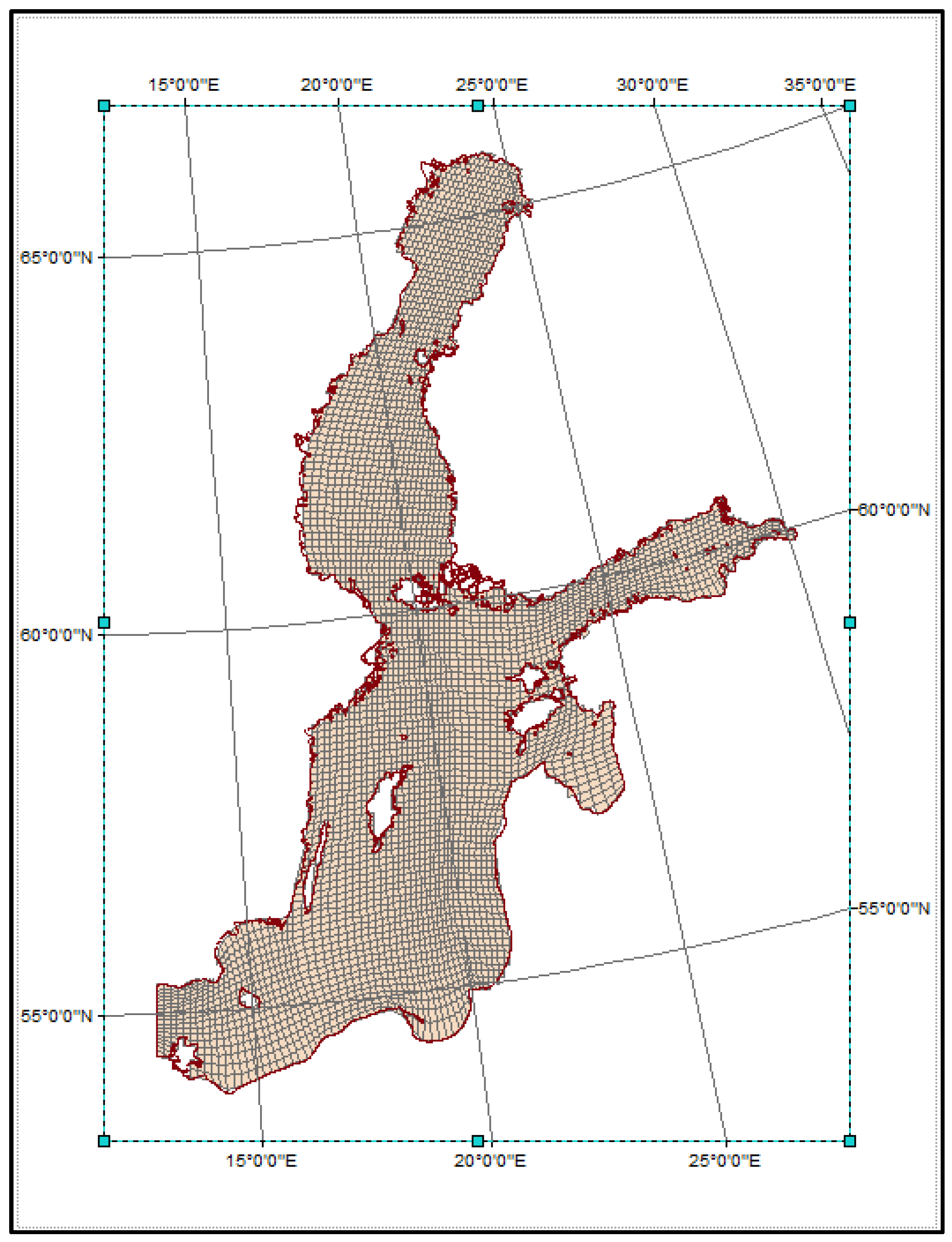
The model grid was created using the grid generator tool of GEMSS
®. A non-uniform boundary-fitted curvilinear grid in a horizontal plane (
x-
y) with a non-uniform
z-layering in the vertical plane was created for the study domain and is shown in
Figure 4. The grid dimensions are 195 × 200, with an approximate cell size of 4.8 km. The final bathymetry described in the previous section was used to interpolate the depths for each grid cell in the study domain. Since depths less than 100 m cover almost 80% of the Baltic Sea, the vertical layers were designed to have a finer resolution within this depth. The total number of vertical layers used in the current study was 47, with thicknesses varying from 1.5 m to 12 m.
2.2.1. Input Data
The model boundary conditions consisted of discharge, head (water levels), precipitation, and meteorological forcing conditions. The true dynamic character of the input data is an important issue that directly affects the results of any hydrodynamic simulations. Here, the input data are the river discharge hydrographs and the forcing meteorological conditions. The amplitude and frequency of the data control various hydrodynamic properties such as stratification and mixing processes. The control file generator tool of GEMSS was used to define all forcing data needed for the current study.
The discharge boundary conditions were defined for 69 rivers out of 72 that enter the modeled region. To define the exact locations of the rivers, a GIS file was used. The river data included the flow discharge, water temperature, and salinity. We assumed that the rivers enter through the water surface grid in the model.
The water level was set at the open boundary with the North Sea, as shown in
Figure 1 with a red line (≈104 km wide). The GPS coordinates are 54°28′ N 12°50′ E and 55°22′ N 13°03′ E in the south and north directions, respectively. To set the water level, the data at the gauge station Skanör (55°26′ N 12°50′ E) were used. At the open boundary the water temperatures and salinity profiles from monitoring station BY1 (see
Figure 3) were used.
The precipitation data in mm/day were applied regionally by dividing the Baltic Sea surface into 19 regions, each with its corresponding rain intensity. Both point and gridded data were used for meteorological forcing conditions. The gridded data cover the whole Baltic drainage basin with a grid of (1° × 1°) squares. The grid extends over the area: Latitude 49.5°–71.5° N, Longitude 7.5°–39.5° E. The gridded data covers 32 years, starting in 1970. The gridded meteorological data represent geostrophic wind and were converted to the open surface wind speed needed for the model using the 2/3 power law. The second set was point data, which are available mainly along the coastlines.
2.2.2. Initialization
The model initialization is an important part of any hydrodynamic simulation, especially in the case of large water bodies such as the Baltic Sea. The long residence times make the model output sensitive to the choice of method. In the present study, we initiated the model using the data available at all the monitoring stations for water temperature and salinity. A total of 22 monitoring stations (see
Figure 3) were used to interpolate temperature and salinity for the entire model grid at the start of the model simulation on 1 January 2000.
2.3. Simulations
In the present study we used the following setups for both partial and complete simulations, i.e., one year and 10 years.
Vertical dispersion: Two-Equations with Mellor–Yamada formulation.
Mixing dispersion: Okubo formulation.
Transport diffusion: Prandtl method.
Surface heat exchange: term by term, defining all the heat source and sink terms with atmospheric interaction.
Transport model: Quick.
Vertical momentum: Non-hydrostatic.
Coriolis force: Using model grid.
The maximum time step used in the model simulations was 360 s. The auto time step feature available in GEMSS
® was used so that the model time step goes only below the maximum time step due to extreme forcing conditions such as large wind speeds and river discharges. The calibration and verification simulations were carried out on a 4.8-km model grid shown in
Figure 4. The model was run for the year 2000 for calibration. The model validation was done for the full 10 years using the restart files created by the calibration run.
4. Discussion
The understanding of stratification in large water bodies is of significant environmental importance due to its direct coupling with water quality dynamics. Severe thermal stratification can have a number of adverse effects, among which are reduced water quality and the spatial distribution of fish [
41]. Any prolonged stratification can reduce oxygen solubility, which leads to oxygen depletion in deep water masses. The deeper water masses in the Baltic Sea are particularly vulnerable to eutrophication below the halocline or in regions affected by thermal stratification [
42]. We know that eutrophication is the most serious and challenging environmental problem for the Baltic Sea [
1]. Consequently, accurate knowledge of stratification dynamics is required for the management of eutrophication in the Baltic Sea.
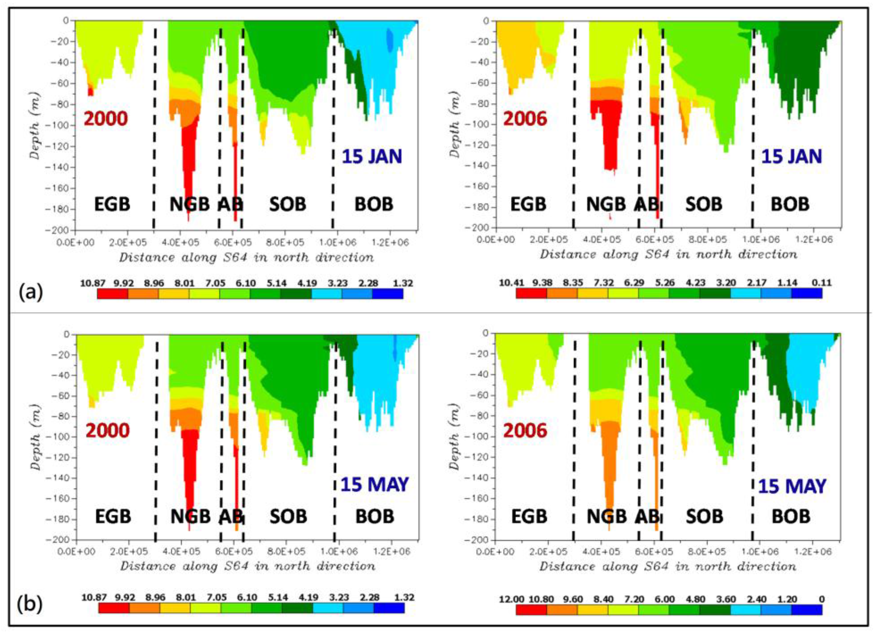
The river Neva, the most voluminous river entering the Gulf of Finland (referred as Gulf in the foregoing discussion) from the eastern coastline (2500 m
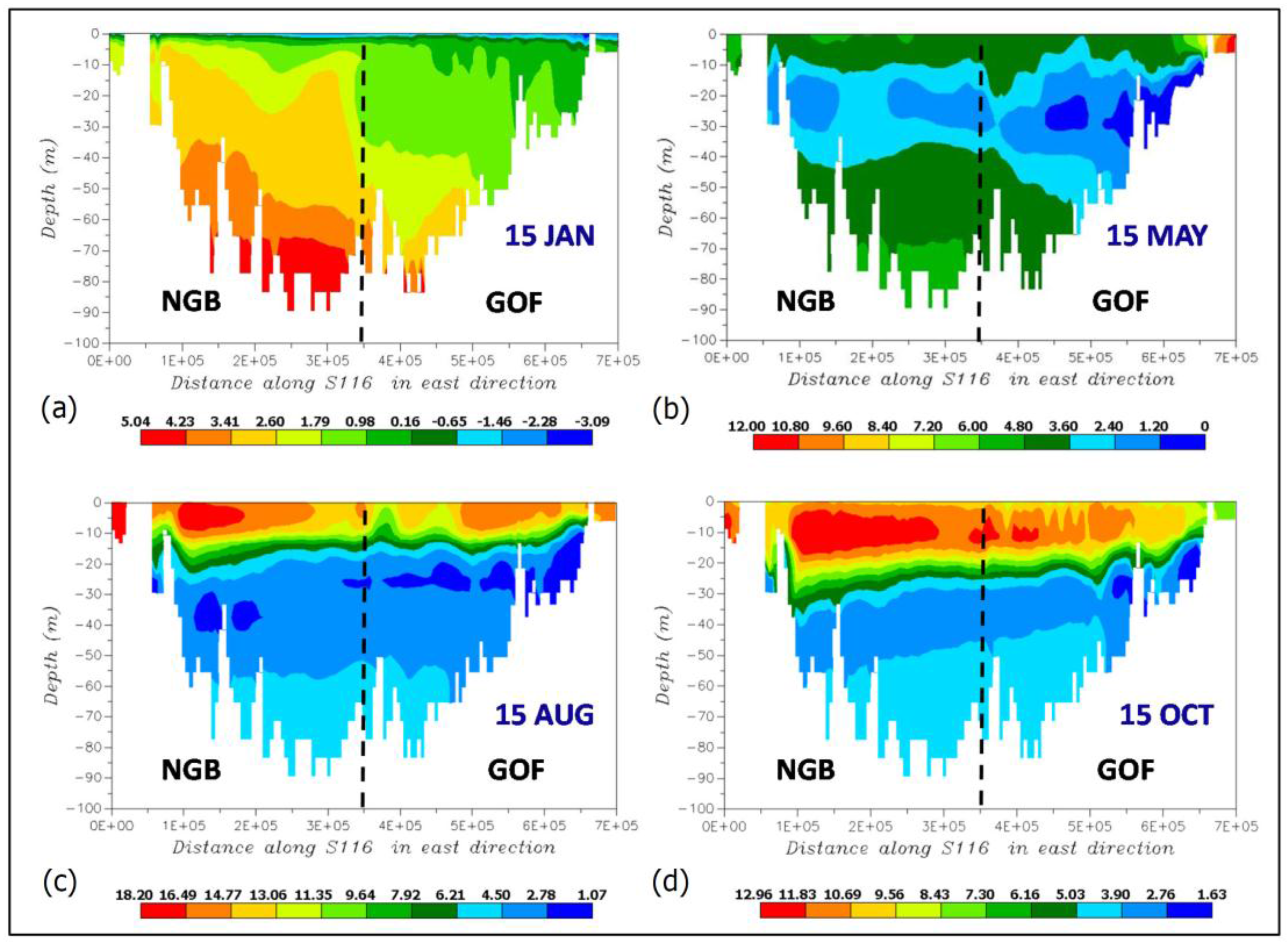
3/s), significantly affects the stratification in the Gulf. The zero-salinity water from the river creates a permanent plume that propagates westwards to a distance of 50–150 km. The plume salinity varies from 0% to 5% and extends to a depth of about 15 m. The maximum extension occurs during early spring periods. The seasonal cross section plots are shown in
Figure 14 at S116 for the year 2000. The stratification in the Neva region appears to have a permanent multi-layer structure with few seasonal variations. The characteristic three-layer structure is found in the inner Gulf region. The stratification characteristics in the Northern Gotland Basin are similar to those in the inner Gulf region. It is interesting to note the significant salinity increase to 9.5% that is confined to the Northern Gotland Basin and the bottom layer.
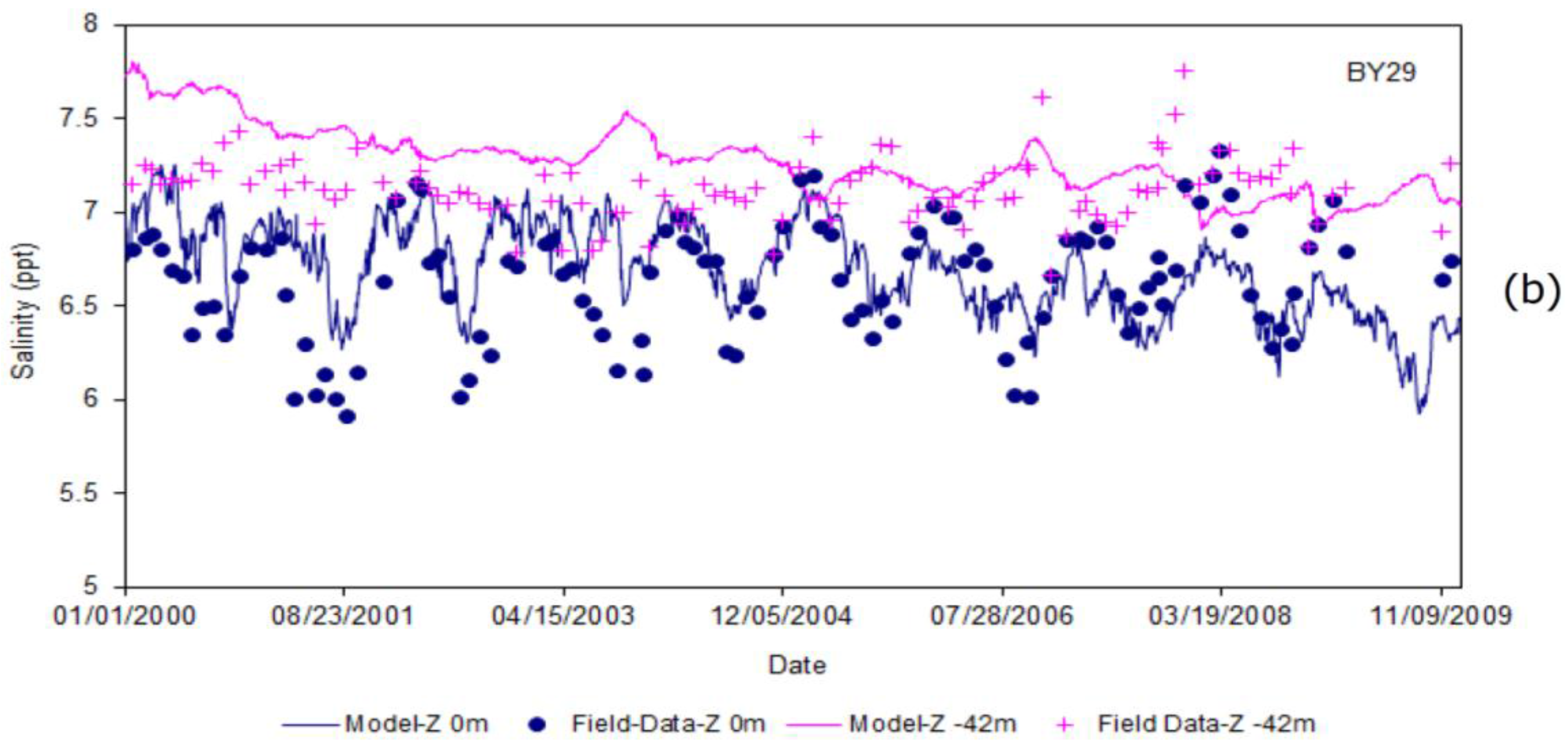
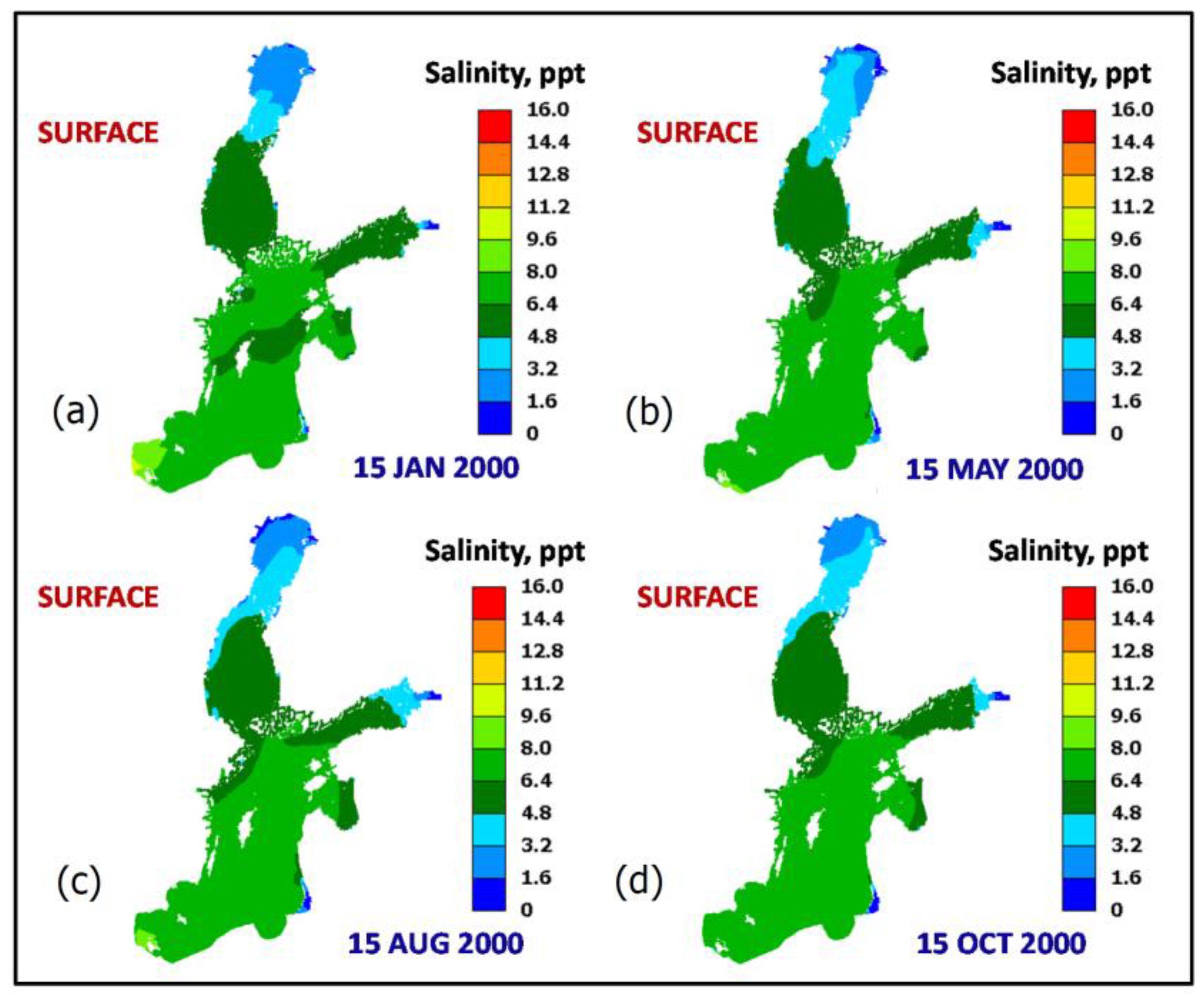
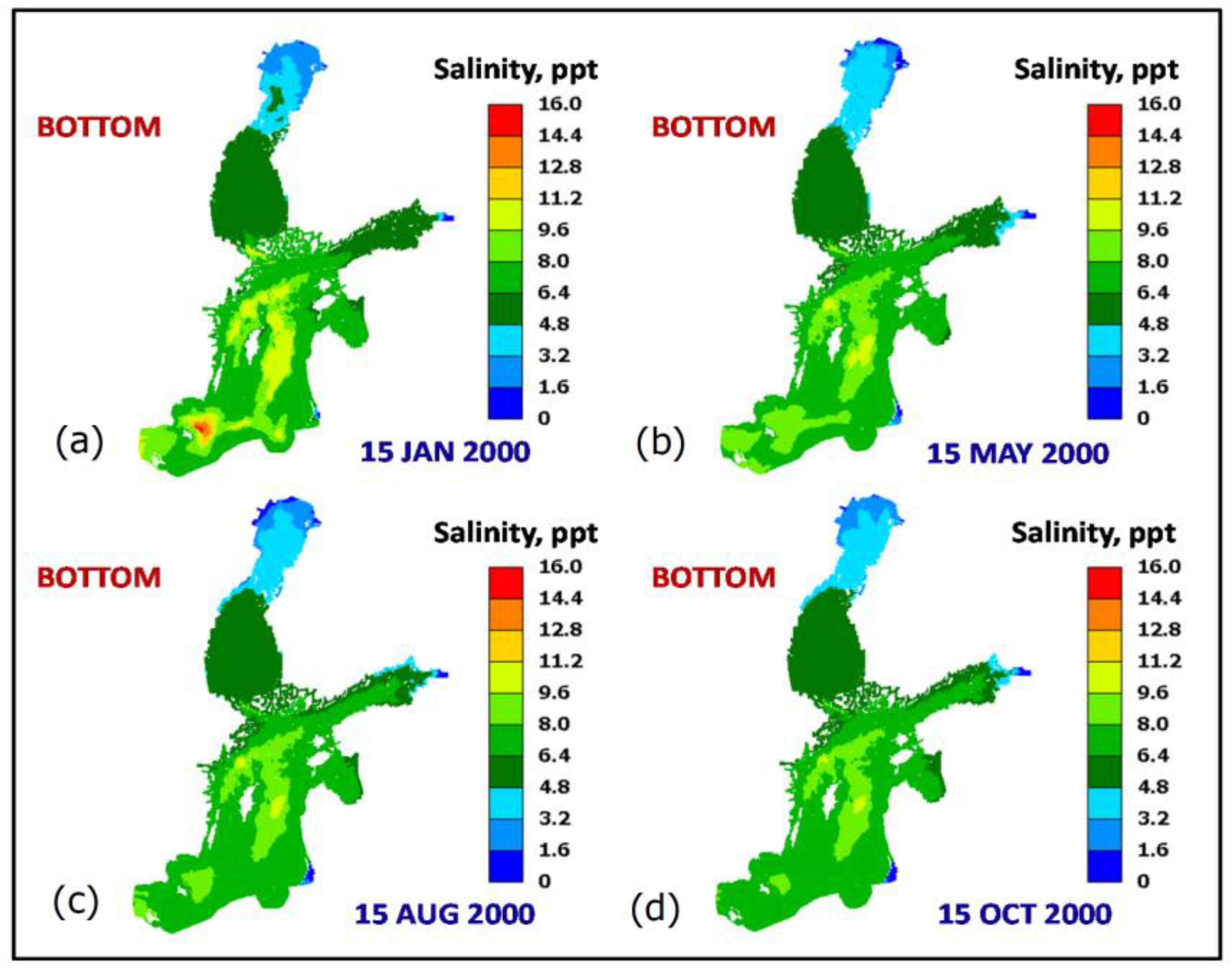
The model prediction of three-layered salinity stratification in all basins of the Baltic Sea is in general agreement with previous studies [
8]. Salinity stratification has a strong seasonal variability but is much weaker than the corresponding variability in temperature. The summary of model-predicted salinity data for the entire 10-year period into seasonal normalized layer thicknesses is shown in
Table 3. The normalized values are more applicable than the absolute values given in the literature as the layer thicknesses could be estimated as a function of depth. The latter vary significantly within and among the basins. To examine the validity of the generalization, we compared the model and measured salinities at all stations and found good agreement between the data. An example is given in
Table 4, which compares model results with measurements at station C3 (located in the Sea of Bothnia; see
Figure 3) for the year 2000. Evidently, the predicted mean thicknesses are within the range of the measured data that supports our generalization.
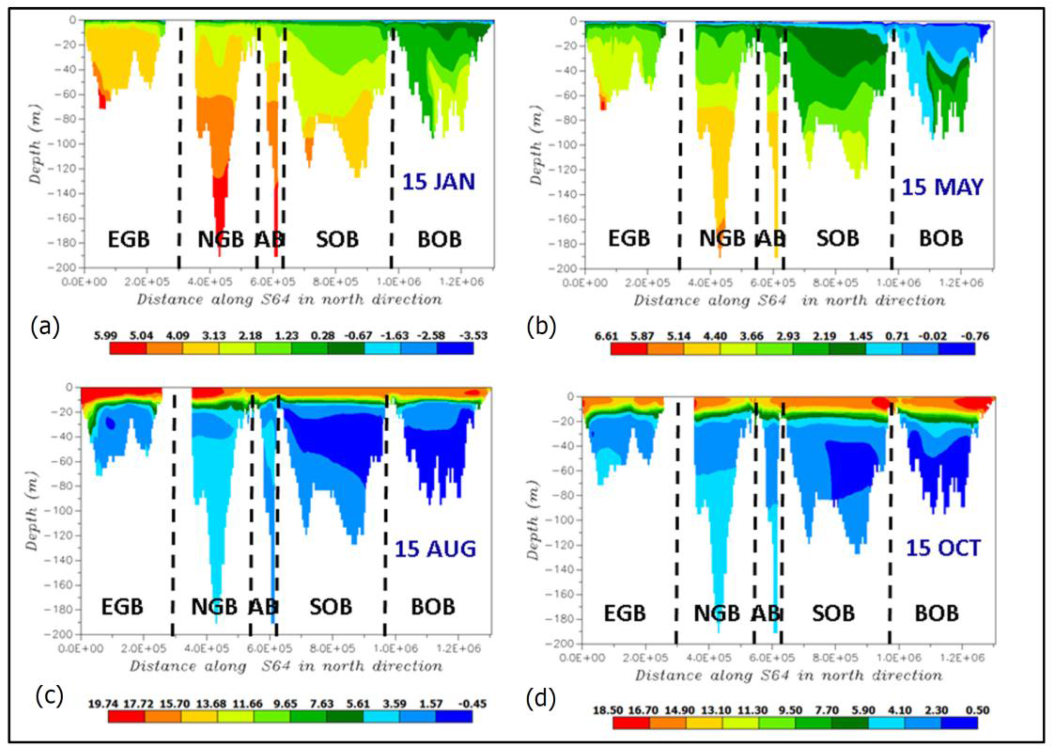
The detailed investigation of thermal stratification for a 10-year period (i.e., 2000–2009) revealed some new features. The current study revealed a multilayered structure that contains several thermocline and dicothermal layers. The statistical analysis of all simulation results made it possible to derive the mean thermal stratification properties, expressed as mean temperatures and the normalized layer thicknesses (
Table 2). The three-layered structure reported by Leppäranta and Myrberg [
7] appears to be oversimplified.
The thermocline layer has a sharp temperature gradient that connects the upper and lower two layers. We have found the three-layer model to be valid only during the winter. In the northern basins, the vertical temperature gradients are significantly lower than for the southern basins (a factor 3). We attribute the difference to the formation of an ice cover during winter and spring in the northern basins (i.e., Northern Gotland Basin and above), which affects the surface heat transfer and its exchange with the overlying cold air. The ice layer acts as a thermal barrier preventing further heat losses due to the action of wind and convective transport. Consequently, the upper layer is rather thick and can occupy up to 65% of the depth in these basins. Following the winter, the three-layered structure is decomposed into several layers with increasing or decreasing temperature gradients. The process takes place in all the basins in the Baltic Sea. Here, we believe the primary driving force is the increased mixing processes between the basins during the ice-free periods. The high-momentum fresh water inflows from the rivers contribute to higher surface water temperatures, thus increasing the temperature gradients. On average, the thickest layer is the bottom layer (≈50%) with a small temperature gradient, except in the Bornholm and Arkona basins. We believe the low gradients are due to low-intensity exchange processes in the northern basin of the deep water regions.
The Bornholm and Arkona basins are shallower and more influenced by the exchange of warmer and more saline waters with the North Sea. This is reflected by the increased temperature gradients in these basins (from ≈0.02 °C/m to ≈0.5 °C/m). Our simulations indicate a wide spectrum in the layering properties among the basins. However, a few generalizations appear to be possible based on the results listed in
Table 2. The thermocline occupies about 25% of the water depth in each basin. The deep bottom layer is about 40% of the water depth with temperatures of about 3 °C and 5 °C in the northern and southern basins, respectively. Our mean results on the properties of thermal stratification agree well with the results reported by Leppäranta and Myrberg [
7]. Here, the reported annual averaged halocline thickness is 10–20 m. For example, in the Bay of Bothnia we get an averaged normalized depth of 35% from
Table 2. The mean depth is 40 m, which yields a thickness of 14 m—well within the range given by Leppäranta and Myrberg [
7].
There is also some evidence of upwelling and downwelling along the coastlines across the Baltic Sea [
3,
6,
39,
43]. The existence of the dicothermal layer is an indication of upwelling. The two features occur as wind causes surface water to diverge (Ekman transport) or converge (downwelling). During both processes, water is either replenished from the deep region or forced downwards [
44]. Consequently, the salinity variations, which are mainly controlled by the water balance, are further modified.
We will also examine the validity of having normalized layer thicknesses (
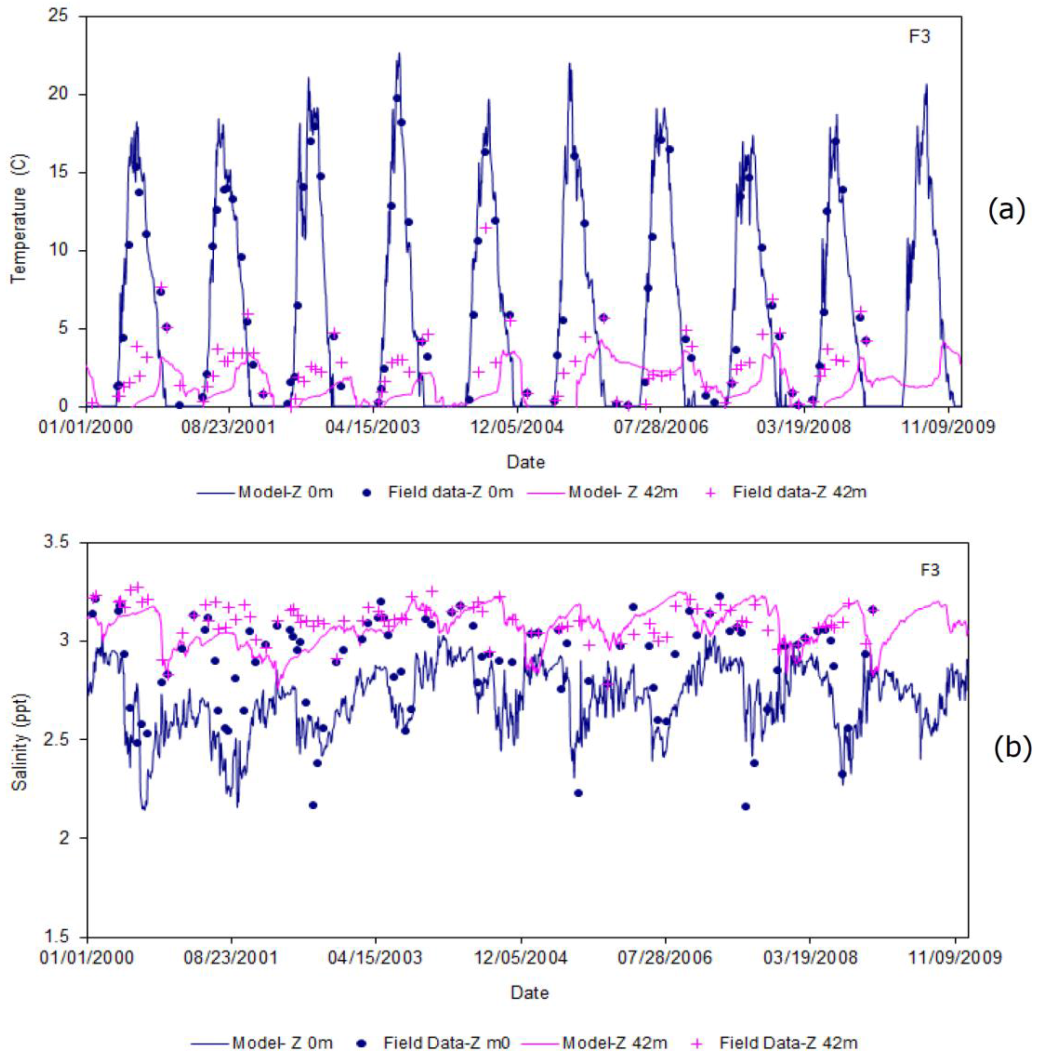
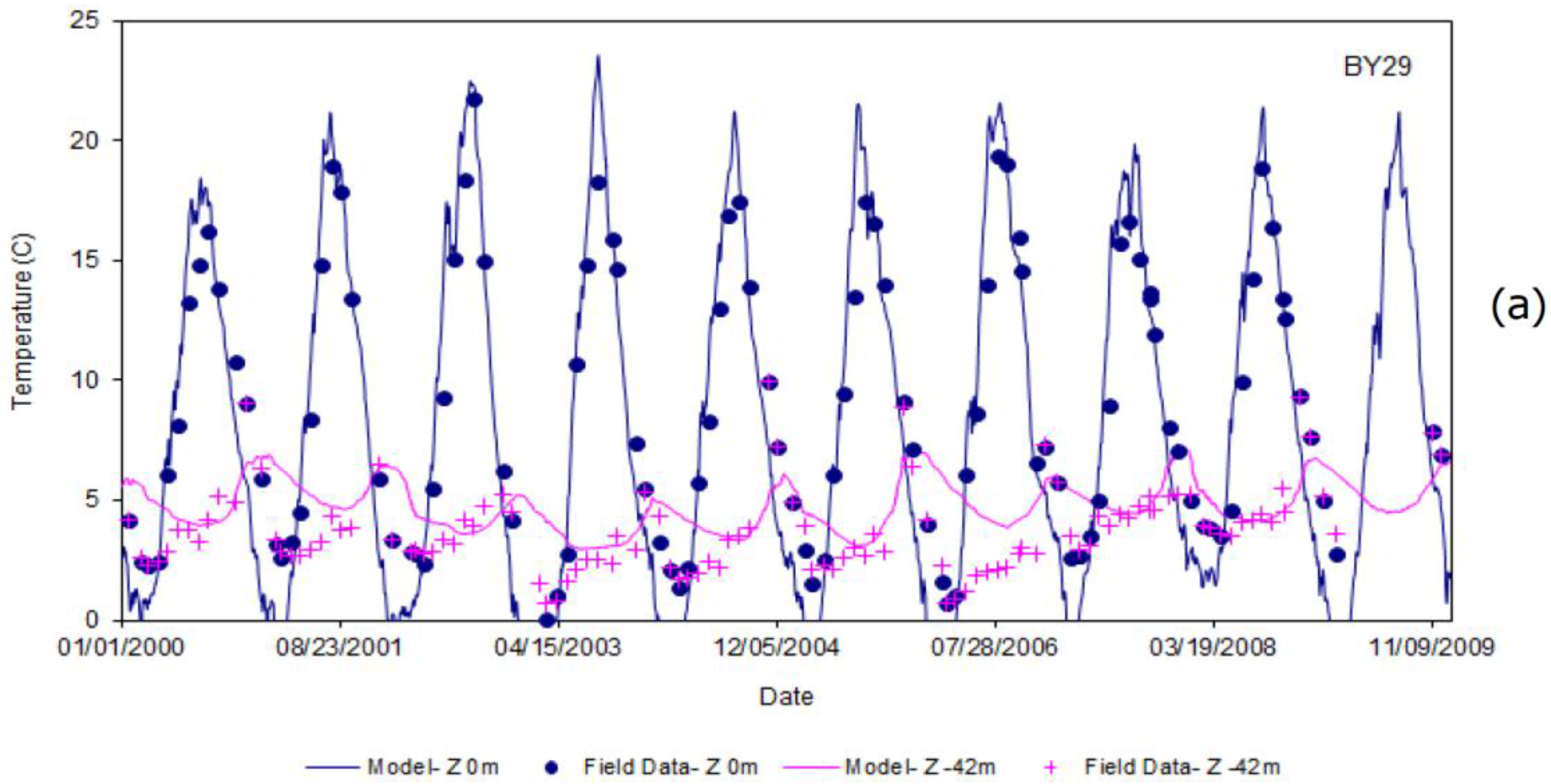
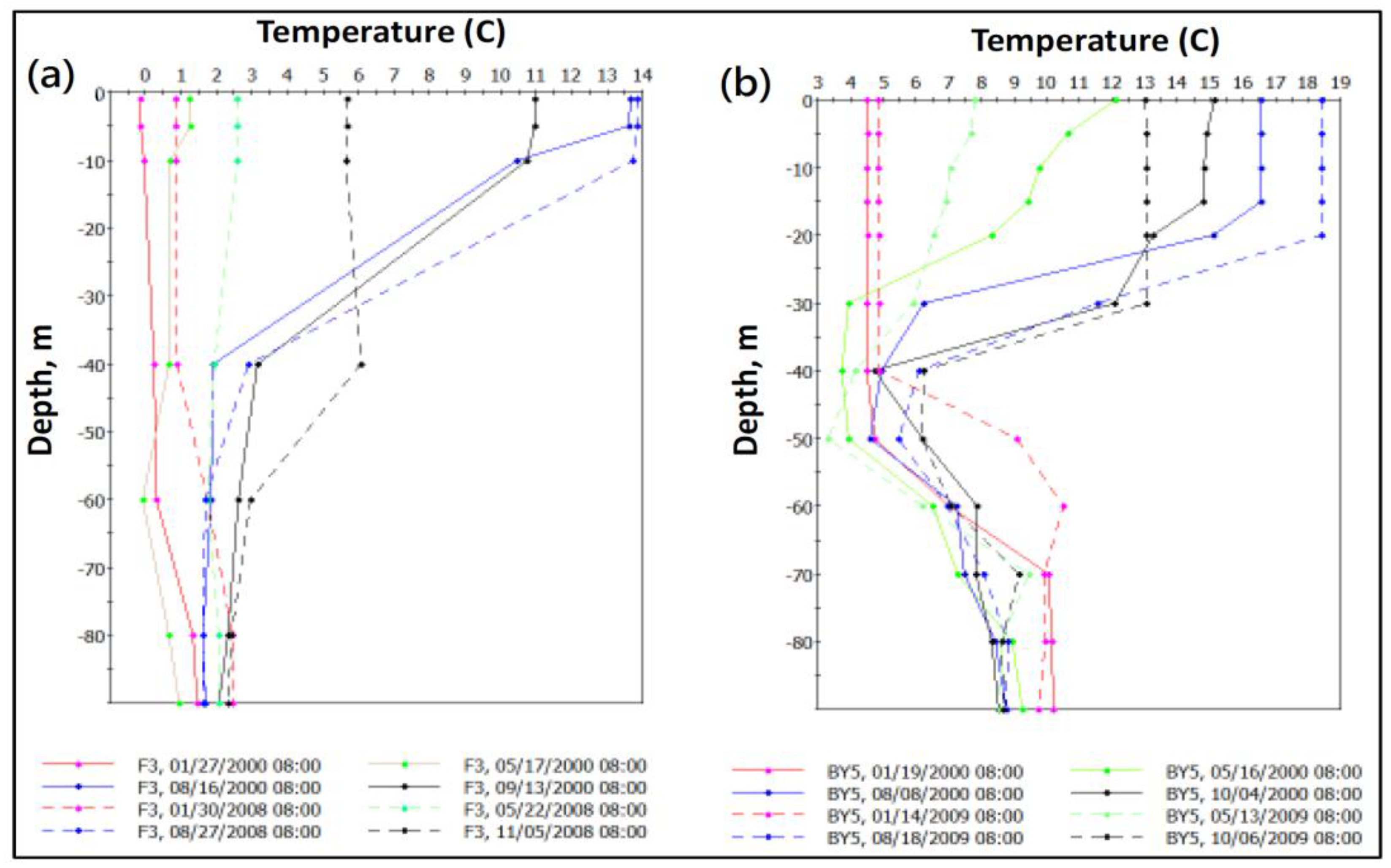
Table 2) in each basin that only vary seasonally. We start by examining the measured vertical temperature profiles for two extreme locations of F3 (Bay of Bothnia) and BY5 (Bornholm Sea).
Figure 19 shows the measured vertical temperature profiles at F3, and BY5 for the years 2000, 2008, and 2009. Note that the data were rather limited and thus the lines are only illustrative and do not necessarily show the correct trends. The good agreement with the simulated summary results listed in
Table 2 is apparent. For example,
Table 2 predicts a thick top layer in the winter period (red line) at both stations that agrees well with the plots for F3, on 27 January 2000, and BY5, on 19 January 2000. We can also note that the profile shapes are preserved during the simulation period. However, the magnitudes of the temperatures show some significant variation. In conclusion, we believe the normalized layer thicknesses give reasonable estimates, with a standard deviation of ±15%.
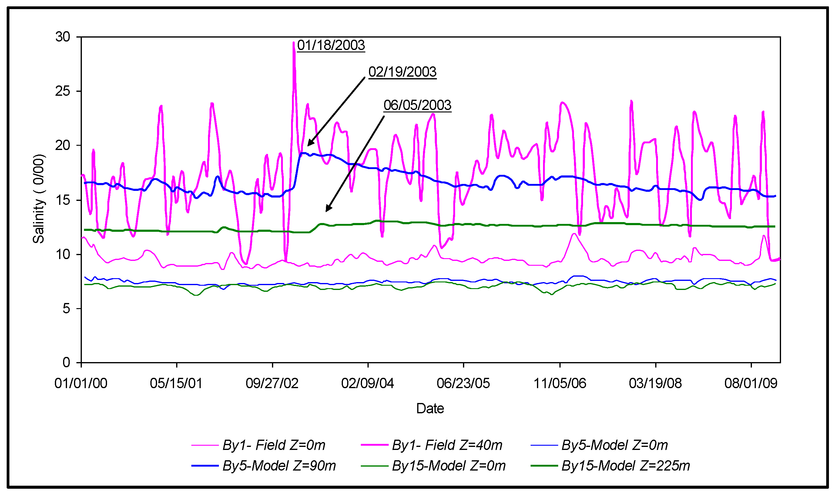
An interesting feature is the extreme inflow event of January 2003. According to Lehmann et al. [
45], a massive salt intrusion of cold and oxygen-rich water from the North Sea took place at Darss Sill, which is a few kilometers west of the open sea boundary used in the model domain (see
Figure 1). They consider the event as “the most important inflow from 1993”. Their results indicate significant changes in both salinity and temperature distributions in the deeper basins of the Baltic Sea. In the present study, we have investigated the reported event by comparing the surface and bottom salinities at all the stations (see
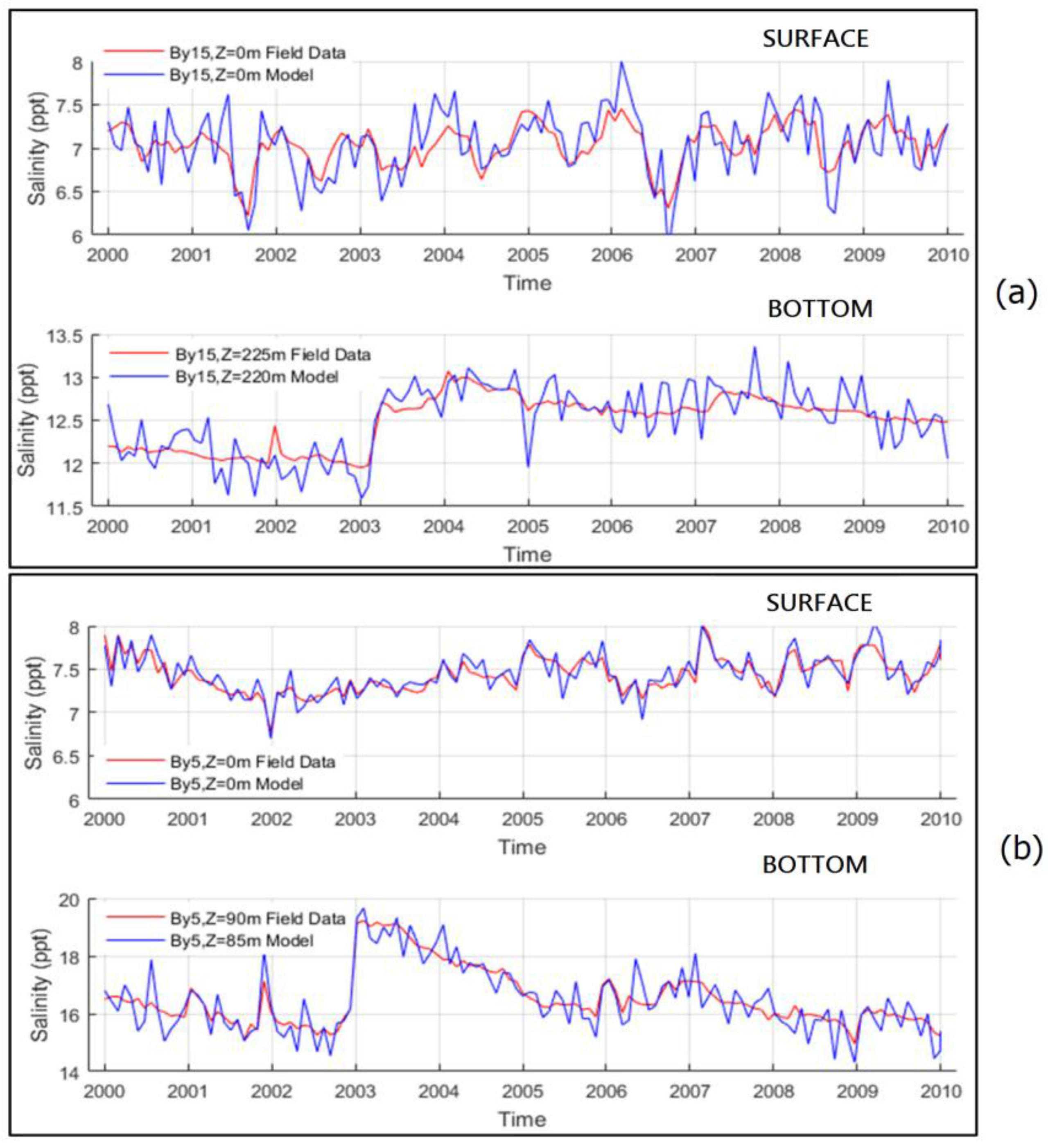
Figure 3). We present the results in
Figure 20, illustrating the salinity time series at stations BY1, BY5, and BY15 at the surface and bottom layers. The curves at BY1 are measured field data but the curves at BY5 and BY15 are model results. The model results are plotted at seven-day intervals for ease of comparison with the field data. Several important features are evident from this figure:
The event took place on 18 January 2003 with a salinity of 29%.
It took nearly a month for the peak salinity to reach station BY5, which dropped to 19%.
The peak salinity was reduced to 12.5% at station BY15 after almost five months.
We computed the horizontal diffusive
and advective transports
using the foregoing information and the distances between the three stations (
Table 5). A representative diffusion coefficient (
) for the Baltic Sea is 10
3 m
2/s [
7]; the advective velocity is typically 0.1 m/s in the Arkona and Bornholm basins (present study). We can conclude that the diffusive transport is much faster than the advective transport. There is a significant reduction in the Eastern Gotland Basin in both modes of transport. It is interesting to note that the temporal variations in the bottom salinity appear to be random as opposed to the surface salinities. The surface salinities have lower amplitudes with no corresponding peaks as the bottom salinity. We believe the outgoing freshwater plays a significant role in lowering the salinity amplitude.
5. Conclusions
An integrated 3D modeling system was developed for the Baltic Sea using a public domain model called GEMSS®. The model was calibrated and verified using 10 years of data covering 2000–2009. We have incorporated boundary conditions and bathymetry with as high an accuracy as possible, to serve as an improvement over previous studies. The model was then used to investigate the vertical structure of the Baltic Sea to understand the stratification and exchange processes across various basins. This paper addressed in detail both the thermal and salinity stratifications, with a focus on the structural properties of the layers.
The hypothesis was that the layer properties could be expressed as dimensionless numbers valid for all seasons. In particular, the detection of cooler regions (dicothermal) within the layer structure has been an important finding. The detailed investigation of thermal stratification for a 10-year period (i.e., 2000–2009) revealed some new features. A multilayered structure that contains several thermocline and dicothermal layers prevails. Statistical analysis of the simulation results made it possible to derive the mean thermal str atification properties, expressed as mean temperatures and the normalized layer thicknesses.
The three-layered structure reported in the literature appears to be rather simplified. The current study found that the three-layer model is valid only during the winter.
The layering properties vary significantly among the basins whereby the layered structure could not be generalized. Nevertheless, a few generalizations appear to be possible. The thermocline occupies about 25% of the water depth in each basin. The deep bottom layer is about 40% of the water depth, with temperatures of about 3 °C and 5 °C in northern and southern basins, respectively.
Three-layered salinity stratification prevails in all basins of the Baltic Sea, in general agreement with previous studies. Salinity stratification has a strong seasonal variability but this is much weaker than the corresponding variability in temperature. We have succeeded in generalizing the seasonal normalized layer thicknesses for the entire 10-year period. The use of normalized values is advantageous compared to the absolute values given in the literature, enabling estimation of layer thickness as a function of depth.
This study provides detailed insight into thermal and salinity stratifications in the Baltic Sea during a recent decade and can be used as a basis for diverse environmental assessments (e.g., anoxia and reduced nutrient mixing between layers [
1]). It extends previous studies on stratification in the Baltic Sea regarding both the extent and the nature of stratification.


