1. Introduction
A vertical datum is a base elevation used as a reference from which to reckon heights or depths. It is called a tidal datum when defined in terms of a certain phase of the tide. For marine applications, tidal datums are the reference planes from which measurements of height and depth are made [
1] and from which marine boundaries are determined. To determine the tidal datum as the reference plane is a challenge. Tidal datum data derived from observed tidal elevation time series are only available in limited locations, where there are at least two to three months or longer of water level time series records. Practically, various deterministic spatial interpolations [
2,
3] can be used to generate a spatially continuous tidal datum distribution over the water. If a hydrodynamic tidal model exists in that region, tidal datums derived from the tidal model can be used as the first estimate field, which is subsequently corrected by adding the correction field interpolated from observation and model discrepancies at the stations.
NOAA’s National Ocean Service (NOS) has developed a software tool called VDatum that provides vertical datum transformations between tidal, orthometric and ellipsoid-based vertical datums [
4]. Over the years, customers and developers of VDatum have raised questions about the uncertainty associated with the VDatum conversions between different vertical datums. Initial efforts were made to quantify uncertainty in both datum transformations and the datums themselves, leading to estimates that could be used for each geographic region represented in VDatum. However, the approach presented here to estimate uncertainties in the tidal datums will provide a path forward in VDatum to eventually be able to provide a more continuous, spatially varying estimate of the uncertainty.
An important part of VDatum’s vertical datum transformations is that the values returned by the VDatum software need to be equivalent to values determined through observations at tide gauge locations. The NOAA/NOS’ Center for Operational Oceanographic Products and Services (CO-OPS) is commissioned to set up the national tidal station network for water level measurements, as well as the establishment of the tidal datum bench marks. The measured tidal datum values at 19 year National Tidal Datum Epoch (NTDE) stations are published in CO-OPS publications and on their website. For consistency, the vertical datum relationships in VDatum need to match the published tidal datum values at the CO-OPS NTDE stations. It is also desirable that the analysis field be close to observed data at CO-OPS non-NTDE stations. This requirement has been one of the guiding principles in the development of the statistical interpolation presented here.
As mentioned, the current tidal datums in the VDatum transformation are computed by integrating modeled and observed tidal datums through a prediction and correction procedure, the latter of which uses a deterministic spatial interpolation method. A solver based on Laplace’s equation is currently used for the spatial interpolation of modeled tidal datum and observed tidal datum discrepancies over the water. The inherent drawback of this spatial interpolation approach is the apparent lack of any physical or statistical principle governing the tidal datums [
3]. Laplace’s interpolation is a low-order interpolation scheme, and the interpolated surface becomes singular at the data points. As a deterministic interpolation method, it is also unable to provide spatially varying uncertainty estimates of the tidal datum product. One alternative for estimating the uncertainty in the tidal datums is to use the delete-one jackknifing method [
3,
5]. Jackknifing has a tendency to overestimate the error and is more appropriate in providing a single-value average estimate of the uncertainty over the whole domain [
3]. The delete-one jackknifing method can provide a good estimate of the uncertainty of the tidal datum product over a large domain, under the condition that the sample size is very large and samples are randomly distributed spatially. However, these conditions are rarely met. As VDatum currently provides single-value uncertainty estimates in the tidal datums for each regional application, the next goal to improve the uncertainty estimates is to provide a spatially varying uncertainty field for each tidal datum. We propose here a statistical interpolation and uncertainty estimation methodology that would provide such a product with spatially varying uncertainty. The interpolation method is derived from the variational principle in data assimilation [
6,
7] by minimizing a cost function, similar to the three-dimensional variational method (3DVAR). The construction of the cost function is such that the discrepancy between (1) the analysis solution that minimizes the cost function and (2) the CO-OPS’ observation values at the observation stations satisfies the constraint that is prescribed by the user. This is achieved by introducing a diagonal weight matrix that regulates the weight of the observed tidal datum error of a particular station in the cost function, therefore also regulating the analysis results. In
Section 2, we will first review the mathematical formulation of the statistical interpolation method and its uncertainty calculation, followed by a description of input matrices in our test case region and the calculation of the error covariance matrices. Results from the test case are presented in
Section 3, followed by a discussion in
Section 4 and the conclusions and recommendations in
Section 5.
2. Method and Data Input
2.1. Method and Mathematical Formulation
Assume that we have a size
n × 1 discrete modeled tidal datum field
fm at model mesh nodes and a size
m × 1 observed tidal datum data set
fo at CO-OPS station locations. Both
fm and
fo follow a normal distribution, and
Var(
fm) =
P,
Var(
fo) =
R respectively. How do we determine a new
n × 1 tidal datum analysis field
f at the model mesh nodes by blending
fm and
fo using a certain criterion? In line with the conventional variational method, we first define a cost function
J(
f), and then solve
f by minimizing the cost function
J(
f). The cost function
J(
f) is defined as
where
H (size
m ×
n) is the interpolation matrix projecting the modeled field to the observed data locations,
W (size
m ×
m) is a diagonal weight matrix that adjusts how much the final product
f differs from the observed values at the station locations. It is assumed the model and observation fields are unbiased. The analysis field
f that minimizes the cost function
J(
f) is
where
is called the gain matrix;
f is the unbiased estimate of the true tidal datum field, and the posterior error covariance matrix
Pa is given by
where
I is the identity matrix.
The weight matrix W provides flexibility and an option if we want the analysis field f to match or be close to the observed values at the observation locations. For a uniform weight distribution W = I, the method is identical to the optimal interpolation (OI) method. The analysis field f at the observed locations can be different from the observed values. If a diagonal element W(i,i) = 0 , then the interpolated values f are forced to match the observed values at the station i, independent of the observed error covariance matrix R.
2.2. Test Case and Input Data
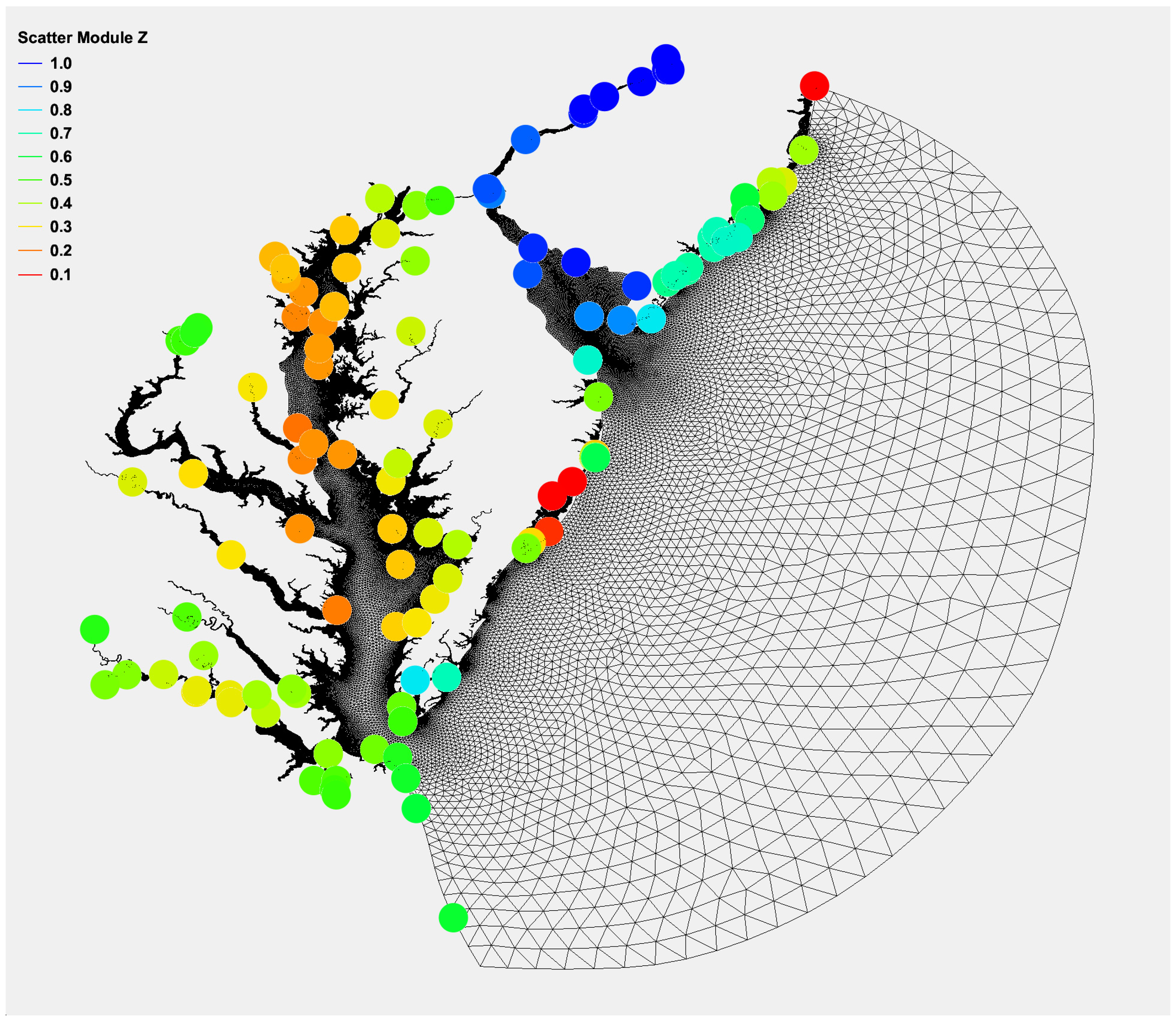
The Chesapeake Bay, Delaware Bay and adjacent coastal ocean (
Figure 1) are used as our test domain to apply the statistical interpolation method to calculate the the Mean Higher High Water (MHHW) tidal datum field and its associated uncertainty field. The Mean High Water (MHW), Mean Low Water (MLW) and Mean Lower Low Water (MLLW) tidal datums are also calculated similarly, but the results will not be presented in this paper. The hydrodynamic tidal model had been developed for the area by Yang et al. [
8] in a previous VDatum tidal model development project. In this section, we will give a detailed description of input matrices in our test case, and the calculation of the error covariance matrices.
2.2.1. Observed Tidal Datums fo and Determination of the Observed Error Covariance R
The observed tidal datums
fo are derived from water level time series collected at the CO-OPS’ tidal gauges. NOS has a standard method to process the time series and calculate the tidal datums [
9]. The observed error covariance matrix
R is a size
m ×
m diagonal matrix. The individual diagonal element of
R is the variance, or the square of the standard deviation, of the observed tidal datum errors. Both the observed tidal datums and the error standard deviations are provided by CO-OPS [
10,
11] following Swanson [
12] and Bodnar’s [
13] formulation.
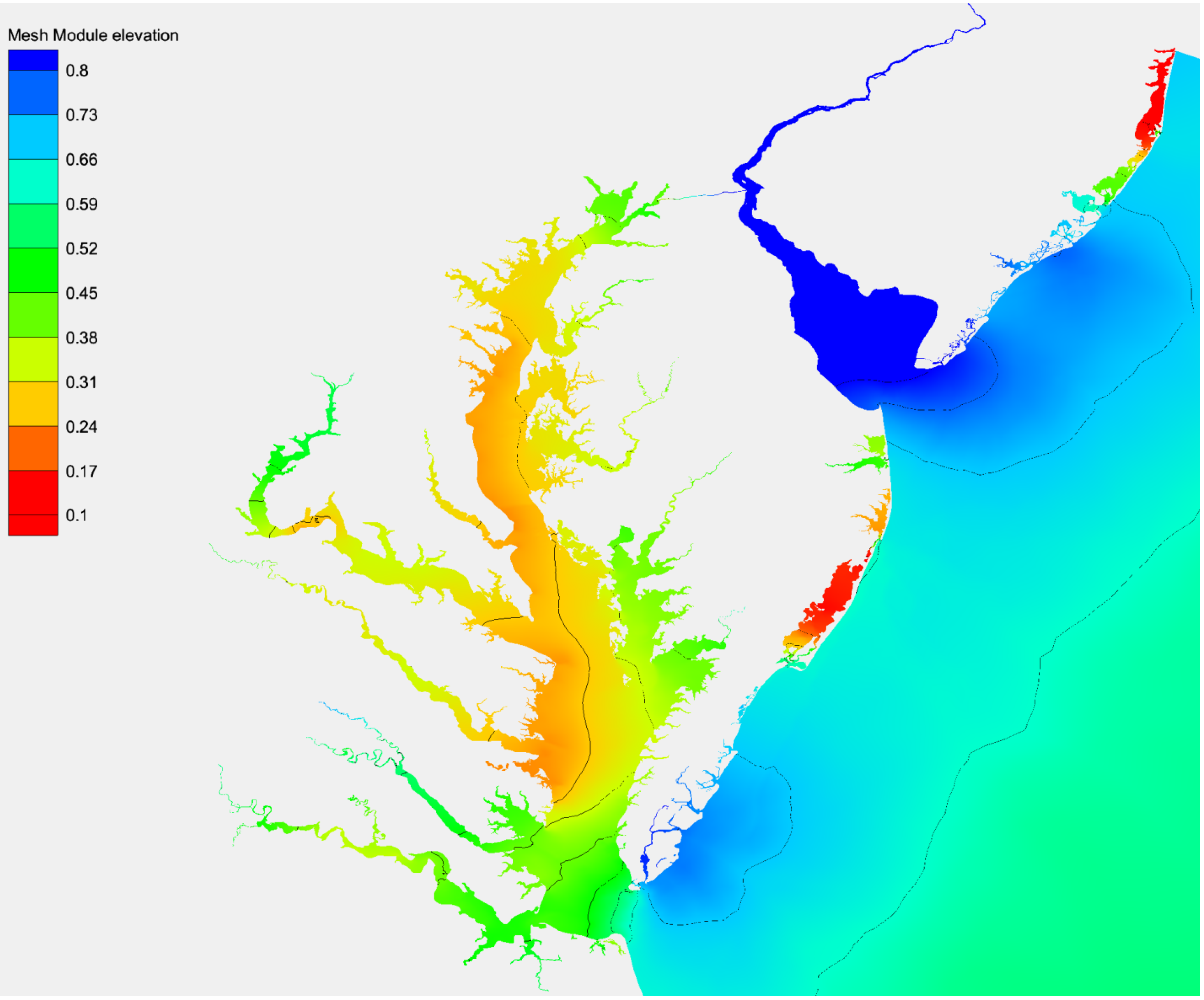
2.2.2. Tidal Datums Derived from the Hydrodynamic Model Time Series fm
If we have a hydrodynamic tidal model, then the tidal datums can be derived from the modeled water level time series using the same process as that used for the observed water level time series [
9]. The biggest advantage of the tidal model is that it provides continuous spatial coverage for coastal and estuarine waters where the navigational safety is mostly of concern. It provides a perfect background tidal datum field (
Figure 2) for model-observation data integration. The hydrodynamic model employed in the tidal simulation to compute the tidal datums here is the ADvanced CIRCulation (ADCIRC) finite element model [
14,
15] in its barotropic two-dimensional depth-integrated (2DDI) mode. The bias of all station model errors is relatively small at 0.41 cm, the maximum absolute error (MAXE) for MHHW is 25.37 cm, the mean absolute error (MAE) is 4.48 cm, and the root mean square error (RMSE) is 6.33 cm (
Table 1).
2.2.3. Model Error Covariance Matrix P
The model error covariance matrix is defined as
Pij = var(
fn1,
fn2) = σ
n1σ
n2corr(
fn1,
fn2), (1 ≤
i,
j ≤
n, unit: m
−2), σ
n1, σ
n2 are standard deviations of the model errors at nodes n
1 and n
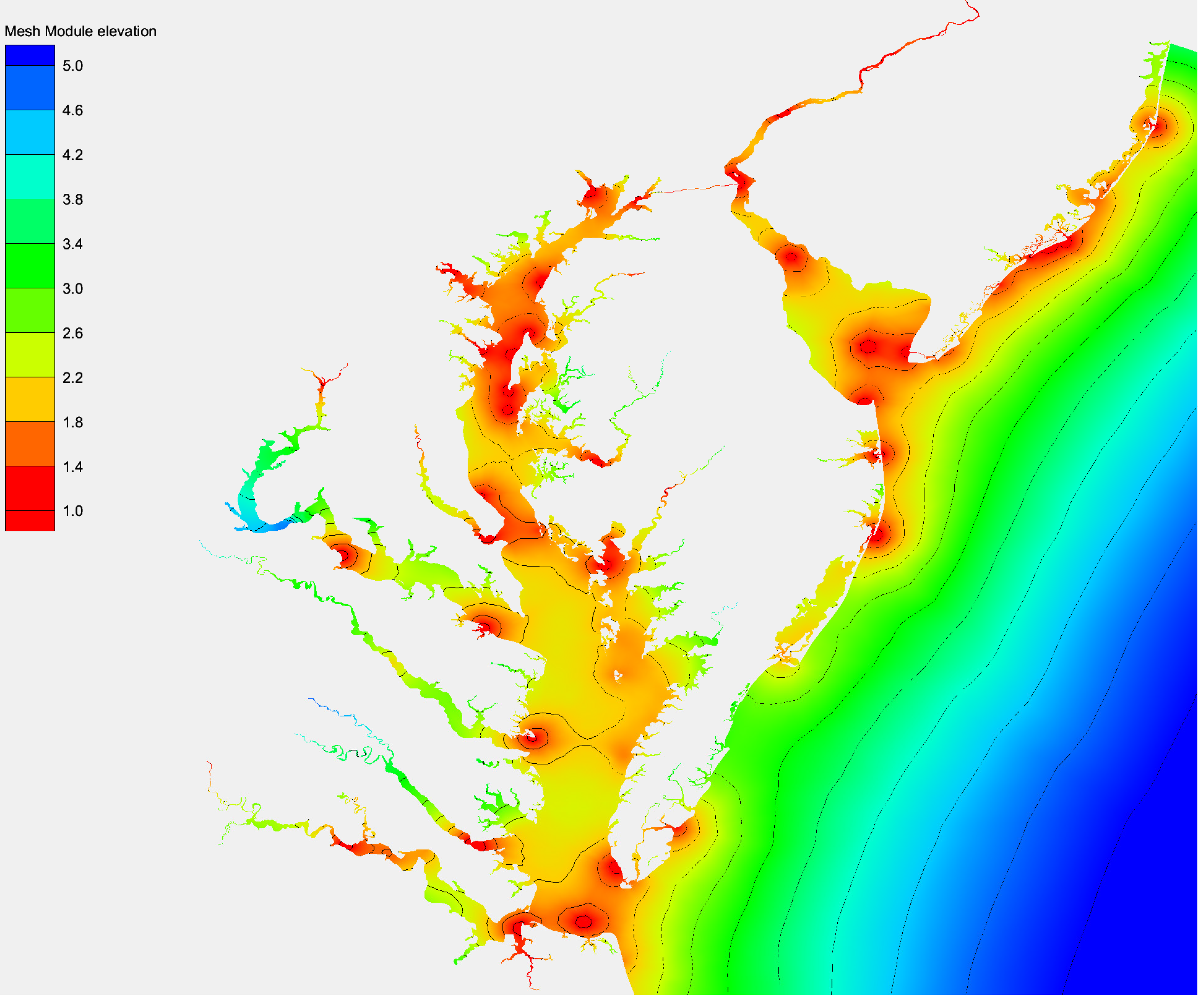
2. The correlation between two points is calculated using a three-day moving average tidal datum time series. The underlying assumption is that the magnitude of the error signal in the tidal datum time series is proportional to the tidal datum signal. Here we give a constant value to σ
n1 and σ
n2, calculated by comparing observed and modeled tidal datum discrepancies over the model domain (
Figure 3). For the Chesapeake and Delaware Bays model, the model error standard deviation is 6.33 cm. The covariance matrix is not related to the distance between node points n
1 and n
2. In an idealized case, it may be true, but in reality the model is not perfect. To limit observation stations far away from the station of interest from interfering with the results, the covariance is adjusted and decreases exponentially over the distance between nodes n
1 and n
2. The relaxation spatial scale for this is 200 km in our application.
2.2.4. Interpolation Matrix, H
The interpolation matrix H is a size m × n matrix projecting the modeled field to the observed data locations; hij (1 ≤ i ≤ m, 1 ≤ j ≤ n, unit: non-dimensional) is the weight of the model nodes j in determining model values at the observation locations i. In our application, we use a linear triangular interpolation to project the model value to the observation location. H is solely determined by the spatial location of the model mesh nodes and observation locations.
2.2.5. Weight Matrix, W
The weight matrix W is a size m × m diagonal matrix determining the weight of R in the computation of the analysis field f. The diagonal element wii (0 ≤ wii ≤ 1, 1 ≤ i ≤ m) is the weight of the observation error variance rii at station i in the determination of analysis field f. If wii = 0, the analysis results will be independent of the observation error at station i. Analysis field f will be the same as the observed value at that station, and the uncertainty will be the same as the CO-OPS assigned value. If wii = 1, then the analysis field will take full account of the error covariance R at station i. The analysis field f will be the local optimal combination of the model results and observations that minimizes the cost function. The posterior uncertainty/error at the station will be reduced, less than both the CO-OPS assigned error and the background model error.
2.2.6. Constraint and Determination of Weight Matrix, W
The constraint that the VDatum technical team adopted for statistical interpolation is simple: the discrepancy between the analysis field and the observations at all subordinate stations should be equal to or less than 1 cm or the CO-OPS’s uncertainty value, whichever is less. The weight matrix W will be determined through iteration following this predetermined constraint.
3. Results
While Equations (2) and (3) provide the general framework of the statistical interpolation, the results can vary depending on the estimation of the observation and model error covariance matrices, as well as on the weight matrix (and constraint) that decides the impact of observed error covariance on the final tidal datum product.
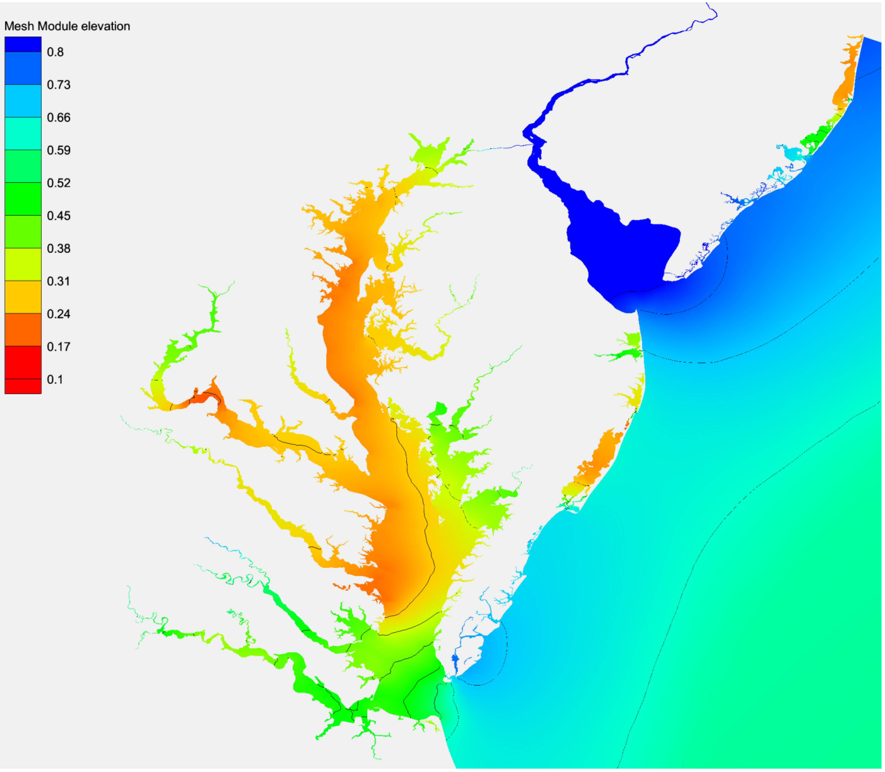
Tidal Datum Analysis Field
The statistical interpolation produces the spatially distributed properties, in this case, MHHW (
Figure 4). The interpolation adjusts the background model values over the whole domain. It corrects apparent discrepancies between observations and model results for MHHW (
Figure 2) at the observation locations by statistically blending the observations and model results. Unless the observed value is 100% accurate (e.g., zero error), the adjusted values will be different from the observed values. The results indicate that the adjustments to MHHW at the stations are very small. The average magnitude of an adjustment is 1 cm, and the maximum adjustment is around 5 cm.
The error statistics, shown in
Table 1, indicate that the statistically interpolated tidal datum MHHW consistently improved all the error measures (bias, MAXE, MAE, and RMSE) in comparison with the modeled and Laplace’s interpolated MHHW.
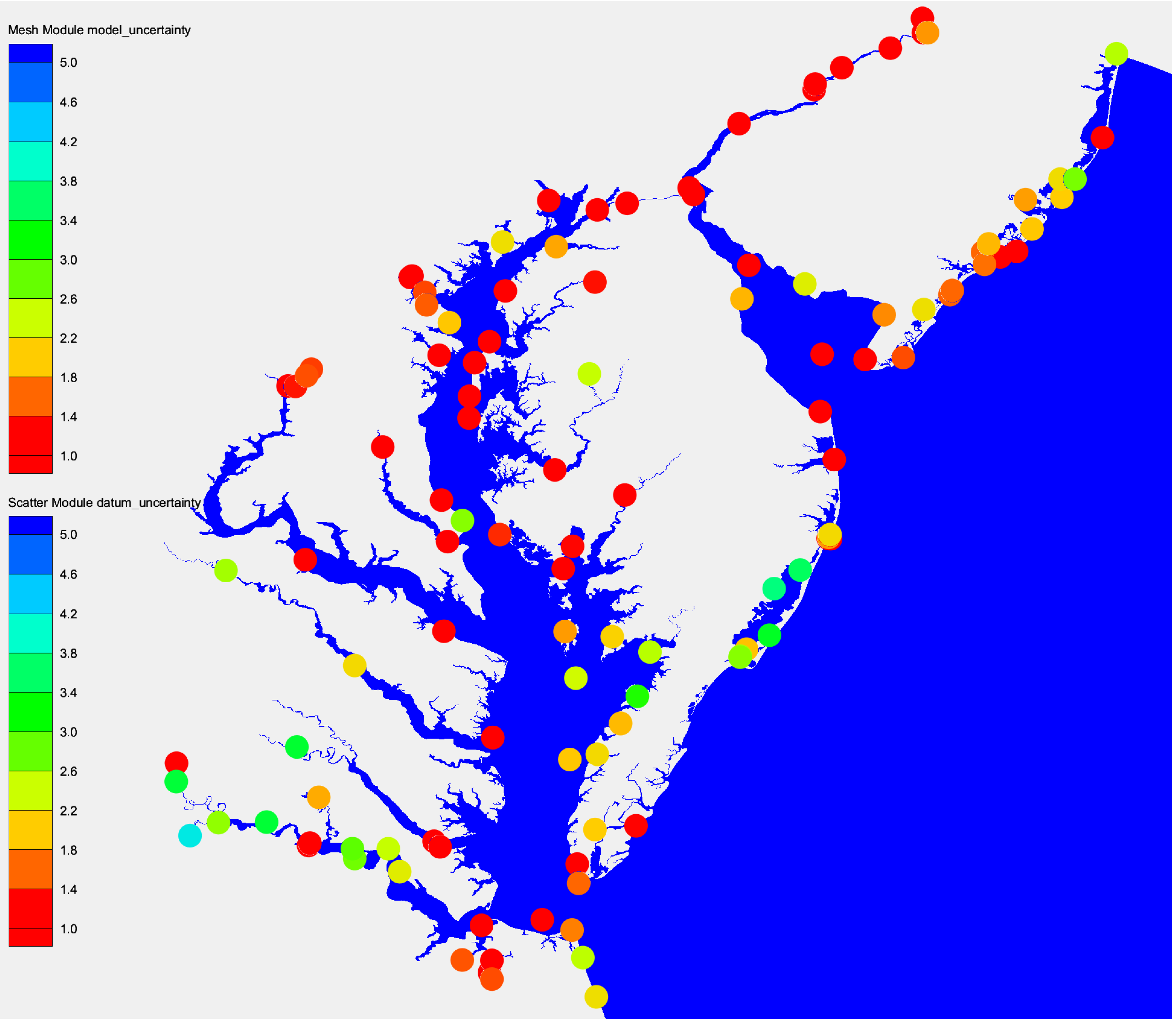
The statistical interpolation not only provides us with the product, but it also produces uncertainty estimates (
Figure 5). The background model uncertainty had been improved dramatically in comparison with the model uncertainty (
Figure 3). The statistical interpolation reduces the uncertainty of the tidal datum product in Chesapeake Bay (which is indicated from the color change under the same color bar), Delaware Bay and the associated coastal areas, and to a lesser extent in the offshore area in the southeast corner of the domain away from the coast where tidal gauge stations are located (
Figure 5).
4. Discussion
The constraint that we adopted is a compromise between an analysis field that matches (
W = 0) CO-OPS’ observed values and a statistically optimal analysis field (
W =
I, statistically optimal implies a lowest overall uncertainty). When we force the analysis field to match all of the observations (
W = 0), the uncertainty at 24 out of 117 total observed data locations is at its highest within the vicinity of those stations (local maxima). That raises a question of whether the inclusion of one particular station into the data assimilation improves the overall results by reducing the uncertainty. The difference between the inclusion and non-inclusion of one particular station into the data assimilation under all matching (
W = 0) and OI cases (
W =
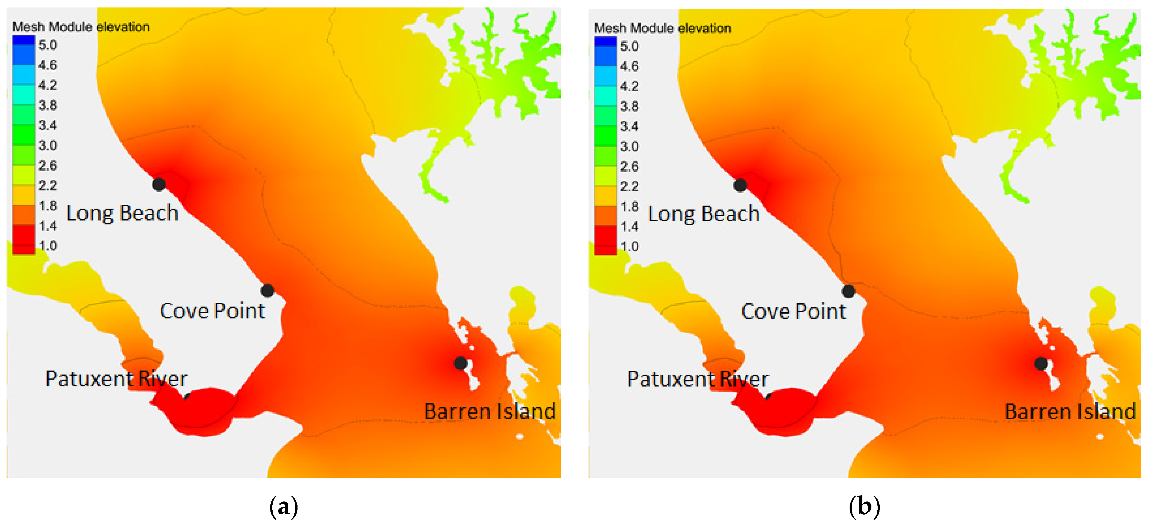
I) can be best illustrated by a simple numerical test to evaluate the differences in the uncertainty fields before and after removing one station in the data assimilation. Here we present the test results for Cove Point (
Figure 6 and
Figure 7), where the CO-OPS’ tidal datum uncertainty is 2.74 cm. Cove Point is one of 24 locations (out of 117) for which the uncertainty at the observed point is at its highest within its vicinity for all matching cases (
W = 0).
Table 2 shows the results from this simple test. For the OI case (
Figure 6), the uncertainty by assimilating the Cove Point data is 1.21 cm, much better than the CO-OPS 2.47 cm uncertainty from the observations (
Figure 6a). Without assimilation, the uncertainty is 1.39 cm (
Figure 6b). For the matching case with the Cove Point data assimilated, the uncertainty at the observed location of Cove Point is given by CO-OPS as 2.47 cm, which is relatively high if compared with its neighboring stations Long Beach and Barren Island (
Figure 7a). Without assimilating the Cove Point data, the uncertainty at that location is 1.40 cm (
Figure 7b). The uncertainty also decreases in the vicinity of Cove Point. Excluding the Cove Point data from assimilation/interpolation is the best option for the matching case. Mathematically/statistically speaking, for the OI case, it can be shown that any data is good data to reduce the uncertainty as long as we know its quality. For the matching case, it is sometimes better to discard a bad data point (although it is still valuable using OI) without assimilation if a neighboring observation is close and good enough to bridge the gap and produce a better result (as shown in the Cove Point case,
Figure 7a,b). If all points match except Cove Point, but Cove Point is still assimilated with (0 ≤
wii ≤ 1), the uncertainty is 1.32 cm. This is lower than the uncertainty (1.40 cm) when Cove Point is not assimilated, and much lower than the CO-OPS uncertainty from the observations (2.74 cm).
The results from further tests of all CO-OPS stations are very clear. For OI, any inclusion of an additional data point will reduce the uncertainty. For the matching case, while for the majority of the data locations the inclusion of data reduces the uncertainty, some do not. The current constraint for statistical interpolation is the compromise reached to minimize the discrepancy between the final tidal datum product and the CO-OPS values. It also provides flexibility in producing a better uncertainty estimate even though it is no longer optimal.
5. Conclusions
In this paper, we propose a generalized statistical interpolation method to integrate modeled tidal datums and observed tidal datums. The interpolation method is derived from the variational method by minimizing a cost function, similar to 3D variational data assimilation. A diagonal weight matrix is introduced to regulate the weight of the observed tidal datum error of a particular station in the cost function, and therefore also in the analysis results. The mathematical formulation of the method derived is more general than Optimal Interpolation (OI) or 3D variational method (3DVAR), but follows very closely the framework of OI and 3DVAR, which is widely used in meteorological and oceanographic applications for model and observation data integration. In a special case, when the weight matrix is an identity matrix, the results are statistically optimal, and the method is identical to OI.
In this application, the setting of the weight matrix follows the constraint that the discrepancy at all stations is less than 1 cm or the CO-OPS’ uncertainty value, whichever is less, and is calculated through an iterative process. The obvious advantage of the statistical interpolation is that the method provides a spatially varying uncertainty of the tidal datum products. Considering that the tidal datum itself is a statistical result from data processing of a long time series, the statistical property calculated from the modeled time series for interpolation is more plausible than any deterministic interpolation. The spatially varying uncertainty can pinpoint regions with low uncertainty levels and help with decision-making on the number and locations of new tidal gauge installations in a geographic area.
From a data assimilation point of view, the statistical interpolation is capable of incorporating all kinds of observed or modeled data with different degrees of uncertainty. The ingestion of additional data will improve the quality and reduce the uncertainty of the product/results.
Our proposed method satisfies our goal to have the tidal datum products be as close to the CO-OPS observations as possible. While it is statistically sub-optimal, it will generally allow the inclusion of any data that will reduce the uncertainty. In our application in the Chesapeake and Delaware Bays, the statistical interpolation in comparison with the raw model output and Laplace’s interpolation reduces the bias, MAXE, MAE, and RMSE. We would strongly recommend statistical interpolation under constraint for tidal datum interpolation in VDatum production. NOAA’s VDatum team has approved this recommendation and accepted the method as the standard procedure for future tidal datum product development.
In the future, the capability of data integration from various sources is probably the most important feature of the statistical interpolation. We expect a steady accumulation of data from various sources (third party observations, different model results). The statistical interpolation or data assimilation provides a perfect framework for data integration. Overall, the statistical interpolation is a better data processing and management tool, and it produces a better tidal datum product with lower uncertainty.
Acknowledgments
Authors would like to thank the NOAA/NOS’ NGS, CO-OPS and OCS VDatum project tri-office management and technical teams’ support of the project. We would also like to thank many experts in and outside of NOAA for going through the project report review process and providing valuable comments and advice to improve the technical report and manuscript.
Author Contributions
L.S. and E.M. conceived and designed the experiments; L.S. performed the experiments and data analysis; L.S. and E.M. drafted the manuscript. Both authors read and approved the final manuscript.
Conflicts of Interest
The authors declare no conflict of interest.
References
- Hicks, S.D. Tidal Datums and Their Uses—A Summary. Shore Beach 1985, 53, 27–32. [Google Scholar]
- Hess, K.W. Spatial Interpolation of Tidal Data in Irregularly-Shaped Coastal Regions by Numerical Solution of Laplace’s Equation. Estuar. Coast. Shelf Sci. 2002, 54, 175–192. [Google Scholar] [CrossRef]
- Shi, L.; Hess, K.; Myers, E. Spatial Interpolation of Tidal Data Using a Multiple-Order Harmonic Equation for Unstructured Grids. Int. J. Geosci. 2013, 4, 1425–1437. [Google Scholar] [CrossRef]
- Hess, K.W.; Kenny, M.; Myers, E. Standard Procedures to Develop and Support NOAA’s Vertical Datum Transformation Tool, VDATUM; NOAA NOS Technical Report; NOAA: Silver Spring, MD, USA, 2012. [Google Scholar]
- Emery, W.J.; Thomson, R.E. Data Analysis Methods in Physical Oceanography; Elsevier Science: Amsterdam, The Netherlands, 2001. [Google Scholar]
- Ide, K.; Courtier, P.; Ghil, M.; Lorenc, A. Unified notation for data assimilation: Operational, sequential and variational. J. Meteor. Soc. Jpn. 1997, 75, 181–189. [Google Scholar]
- Lorenc, A.C. Development of an operational variational assimilation scheme. J. Meteor. Soc. Jpn. 1997, 75, 339–346. [Google Scholar]
- Yang, Z.; Myers, E.P.; Wong, A.M.; White, S.A. VDatum for Chesapeake Bay, Delaware Bay, and Adjacent Coastal Water Areas: Tidal Datums and Sea Surface Topography. Available online: http://vdatum.noaa.gov/download/publications/TM_NOS-CS15_FY08_26_Yang_VDatumCHES-DEL.pdf (accessed on 19 September 2016).
- Scherer, W.; Stoney, W.M.; Mero, T.N.; O′Hargan, M.; Gibson, W.M.; Hubbard, J.R.; Weiss, M.I.; Varmer, O.; Via, B.; Frilot, D.M.; et al. Tidal Datums and Their Applications; Gill, S.K., Schultz, J.R., Eds.; NOAA Special Publication: Rockville, MD, USA, 2001. [Google Scholar]
- Gill, S.K.; Fisher, K.M. A Network Gaps Analysis for the National Water Level Observation Network. Available online: http://tidesandcurrents.noaa.gov/publications/Technical_Memorandum_NOS_COOPS_0048.pdf (accessed on 19 September 2016).
- Michalski, M. USA_MD_Report: Tide Station, Tidal Datum and Geodetic Datum Assessment for VDatum Project; NOAA: Silver Spring, MD, USA, 2011. [Google Scholar]
- Swanson, R.L. Variability of Tidal Datums and Accuracy in Determining Datums from Short Series of Observations; U.S. Department of Commerce, NOAA, NOS: Rockville, MD, USA, 1974. [Google Scholar]
- Bodnar, A.N. Estimating accuracies of tidal datums from short term observations. Available online: https://tidesandcurrents.noaa.gov/publications/NOAA_Technical_Report_NOS_COOPS_077.pdf (accessed on 19 September 2016).
- Luettich, R.A.; Westerink, J.J.; Scheffner, N.W. ADCIRC: An Advanced Three-Dimensional Circulation Model of Shelves, Coasts, and Estuaries, Report 1: Theory and methodology of ADCIRC-2DDI and ADCIRC-3DL. Available online: http://citeseerx.ist.psu.edu/viewdoc/download?doi=10.1.1.472.429&rep=rep1&type=pdf (accessed on 19 September 2016).
- Luettich, R.A.; Westerink, J.J. Formulation and Numerical Implementation of the 2D/3D ADCIRC Finite Element Model version 44.XX. Available online: http://citeseerx.ist.psu.edu/viewdoc/download?doi=10.1.1.675.3043&rep=rep1&type=pdf (accessed on 19 September 2016).
© 2016 by the authors; licensee MDPI, Basel, Switzerland. This article is an open access article distributed under the terms and conditions of the Creative Commons Attribution license ( http://creativecommons.org/licenses/by/4.0/).


