1. Introduction
Accurate determination of water depth is important for monitoring underwater topography and detection of moved sediments, and for producing nautical charts in support of navigation [
1]. Water depth information is fundamental in discriminating and characterizing coral reef habitats, and allows estimation of bottom albedo, which can improve benthic habitat mapping [
2]. The use of satellite and airborne sensors in shallow waters is complicated by the combined atmospheric, water, and bottom signals. This includes variability in the signal from water column scattering and absorption due to dissolved and suspended materials (
i.e., sediments, chlorophyll, and colored dissolved organic matter). Some of these limitations have been overcome by the introduction of high-resolution multispectral sensors that use light reflected from the seafloor to extract benthic information [
3,
4].
Previous researchers have mapped water depth but, in many cases, the methods that were used required the input of known depth values [
5], or assumptions that a pair of spectral bands can be identified such that the ratio of the reflectance in these two bands was the same for all bottom types [
6]. The limitations and validity of obtaining water depth from passive sensors was demonstrated by Maritorena
et al. [
7]. Lyzenga [
8] further enhanced the methodology using multiple linear regressions, which required knowing the optical properties of the water at the time of image acquisition. Stumpf [
9] expanded on the strategy developed by Lyzenga [
5] of using the blue/green spectral bands for depth estimates by reducing the number of parameters that needed to be estimated. The ratio transform proposed by Stumpf [
9] assumed that depth-driven change is significantly larger than the corresponding benthic albedo-driven change. These authors used the ratio transform with two Ikonos satellite sensor wavebands, characterized by differential water attenuation.
Mishra [
10,
11] estimated water depth for each pixel based on a site-specific polynomial model using high-resolution multispectral IKONOS data in a site near Roatan Island, Honduras. A ratio of wavebands (blue and green) were identified that were constant for all bottom types, and it was found that the correlation coefficient between actual depth and estimated depth was 0.94 m, with a Root Mean Square Error (RMSE) of 2.71 m. Based on this approach, the model overestimated depths beyond 21 m.
Collin and Hench [
12] presented another approach in which water depth was retrieved from the WV2 imagery based on different band combinations from all bands (including 5 visible bands) provided by the sensor. This built on the Stumpf [
10] method by enhancing the digital depth models and increasing the range of depth estimation by testing different atmospheric corrections and spatial resolutions.
Hyperspectral sensors have been used to derive properties of the water column and bottom, which includes bottom albedo and water depths. The Airborne Visible Infrared Image Spectrometer (AVIRIS) hyperspectral sensor was used to obtain water depth as well as other properties based on model-derived image optimization techniques [
13]. The results suggested that the model and methods work well for extracting subsurface water properties and demonstrated that the model-derived depths agree with depths measured from 0 to 4.6 m. The AVIRIS sensor was also used in deriving bottom depths in a shallow water marine environment utilizing a remote sensing reflectance model and comparing the model-derived depths to high-resolution LiDAR bathymetry data [
4]. The method is based on the assumption that the use of two bands allows separation of variations in depth from variations in bottom albedo and compensates implicitly for variable bottom [
11].
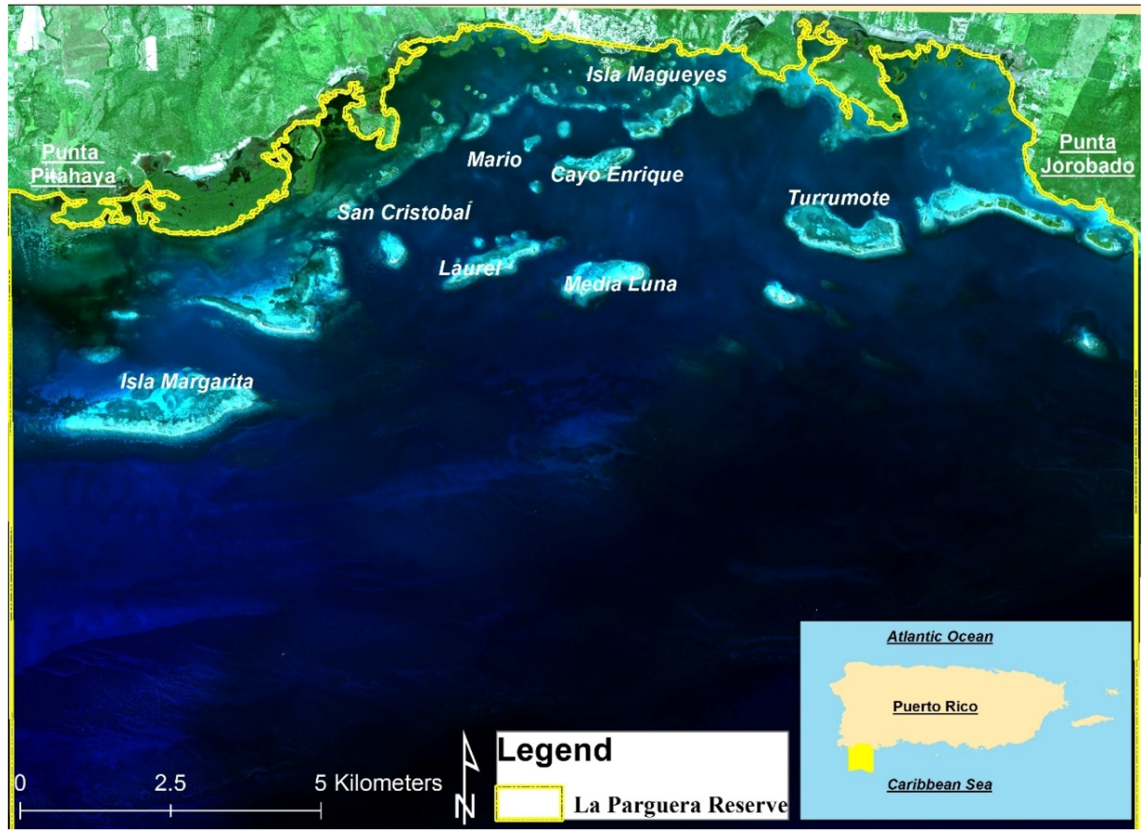
Bathymetric maps for our study area, La Parguera Reserve in southwestern Puerto Rico, have relied on active sensors such as airborne LiDAR and ship acoustic surveys. The use of active sensors were mainly focused in coral reef mapping using side scan sonar [
14] comparison of active sensors (LiDAR and multibeam sonar) for coral reef mapping [
15], or to develop morphometrics from LiDAR to predict the diversity and abundance of fish and corals [
16]. Torres-Madronero [
17] performed a fusion of Airborne Imaging Spectrometer for Applications AISA hyperspectral data and LiDAR SHOALS using Lee’s bio-optical model [
13] to derive depths and other water and bottom optical properties for a coral reef within our study area. This was the only study that used passive sensors to derive bottom depth but only focused on a small offshore cay within the La Parguera Reserve.
The present work has similarities as well as differences in the methods utilized from previous remote sensing-derived bathymetry approaches. This study presents the first high-resolution, large-scale water depth map for La Parguera Reserve derived from passive sensors. This bathymetric map was developed to a significant high spatial resolution (four meters) and was validated using bathymetric data from an active sensor (LiDAR). The project includes an analysis of methods and sensors to derive optimum bathymetry values from passive sensors and the influence of atmospheric corrections in depth retrievals that can be implemented throughout the Caribbean Region and elsewhere.
4. Results
4.1. Atmospheric Corrections
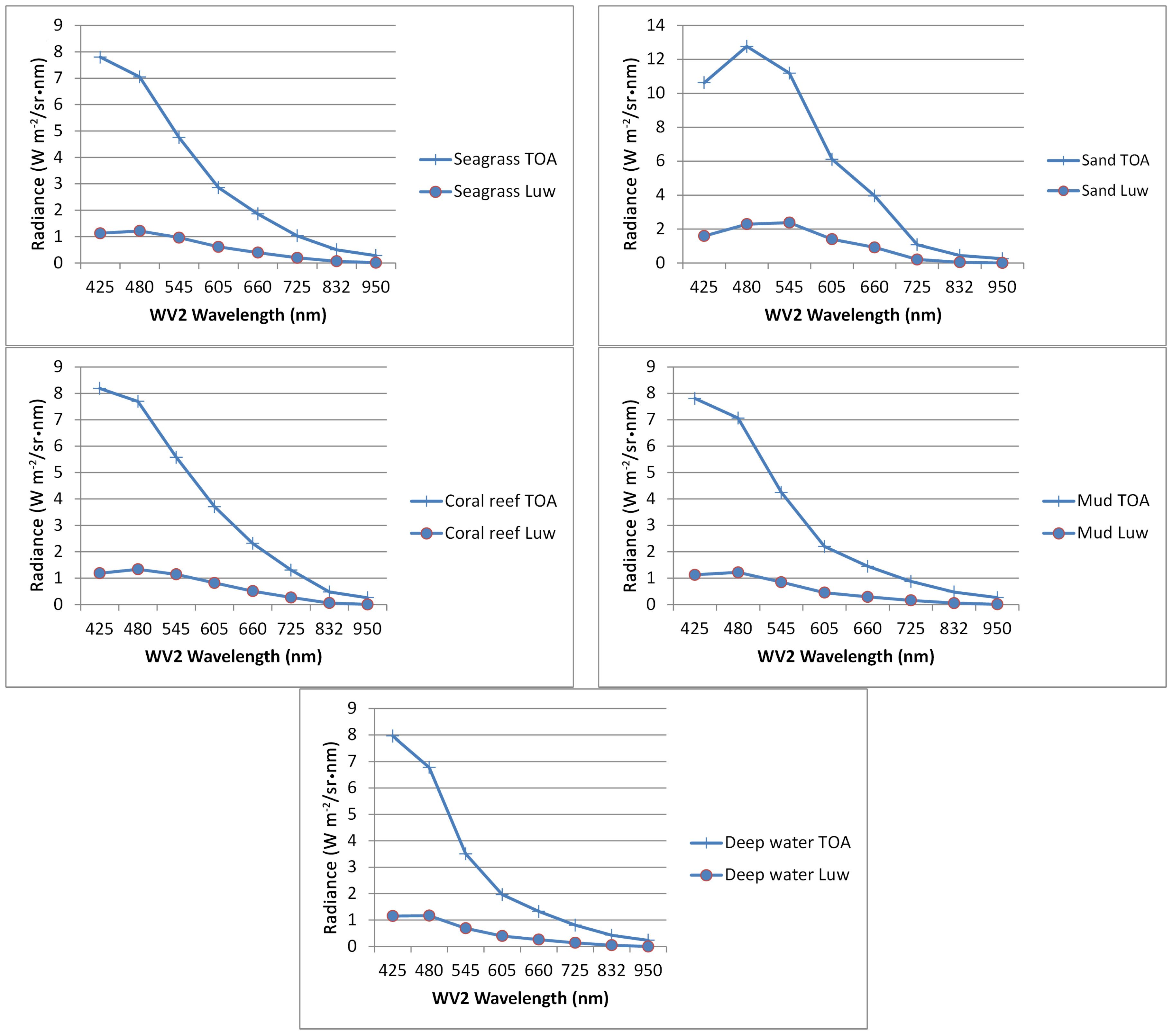
To evaluate the atmospheric influence in the remote sensed signal, radiance values of water over different bottom types were analyzed before and after the atmospheric correction. These bottom types included seagrass, sand, corals, mud and deep-water areas (
Figure 4). The results after the atmospheric correction show that sand had the highest values when compared to other substrates (e.g., coral, seagrass, mud). The atmospheric contribution to the radiance signal for all substrates was estimated at 83% and the “coastal blue”, blue and green bands were found to have the highest values after atmospheric correction, while the near infrared band values were all reduced to near zero.
Figure 4.
Comparison of top of atmosphere (TOA) and water leaving radiances (Luw) derived from WV2 image over different substrates that include seagrass, sand, coral reef, mud and deep water after the CSA atmospheric correction. Notice that the scale in the y-axis of the sand graph is higher.
Figure 4.
Comparison of top of atmosphere (TOA) and water leaving radiances (Luw) derived from WV2 image over different substrates that include seagrass, sand, coral reef, mud and deep water after the CSA atmospheric correction. Notice that the scale in the y-axis of the sand graph is higher.
4.2. LiDAR Depths
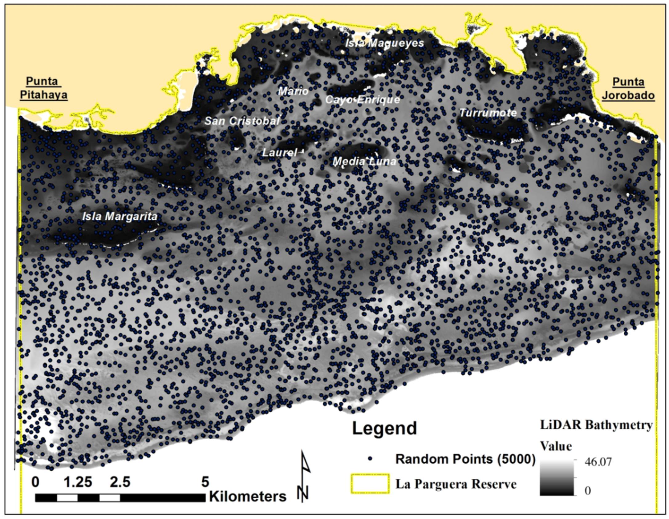
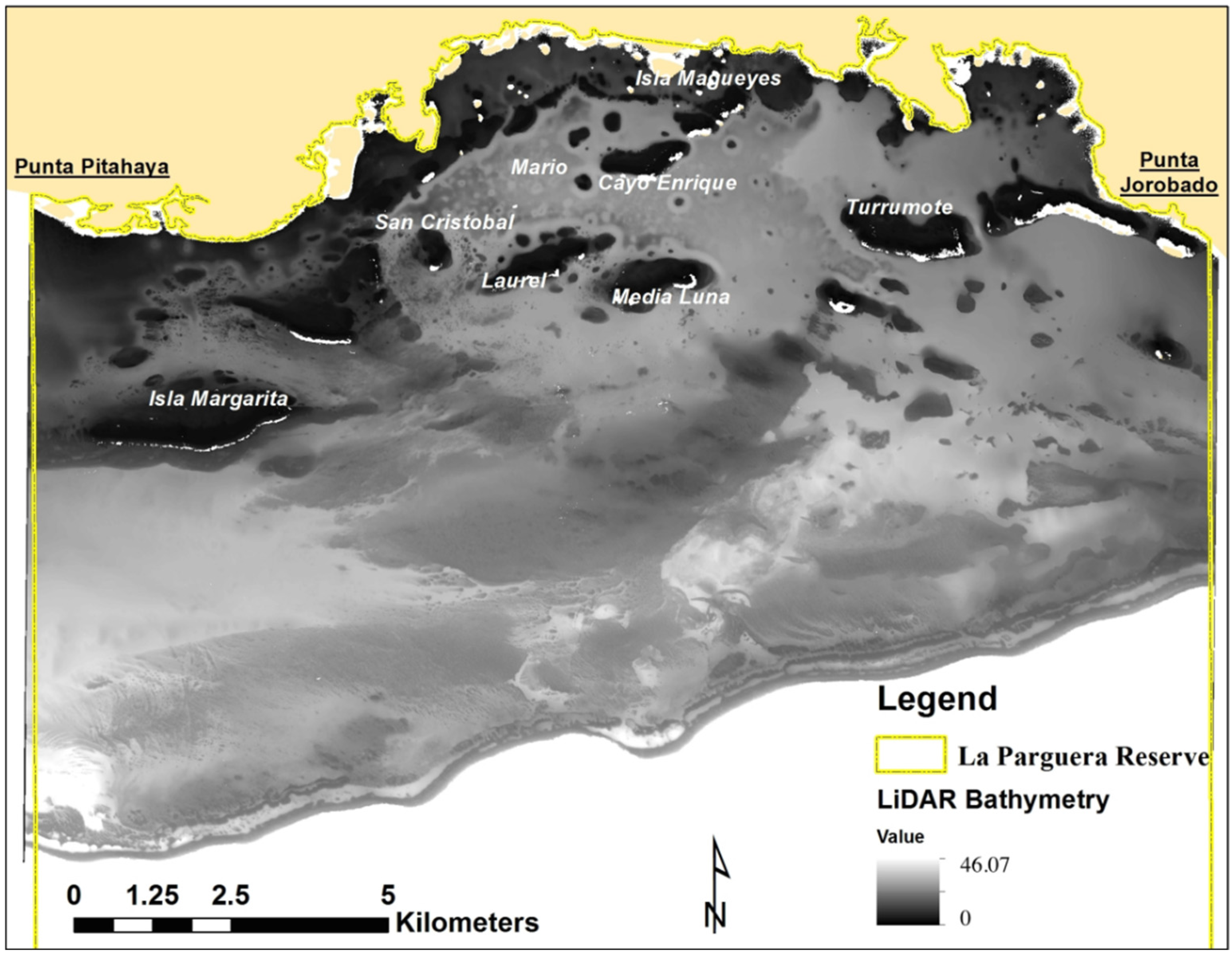
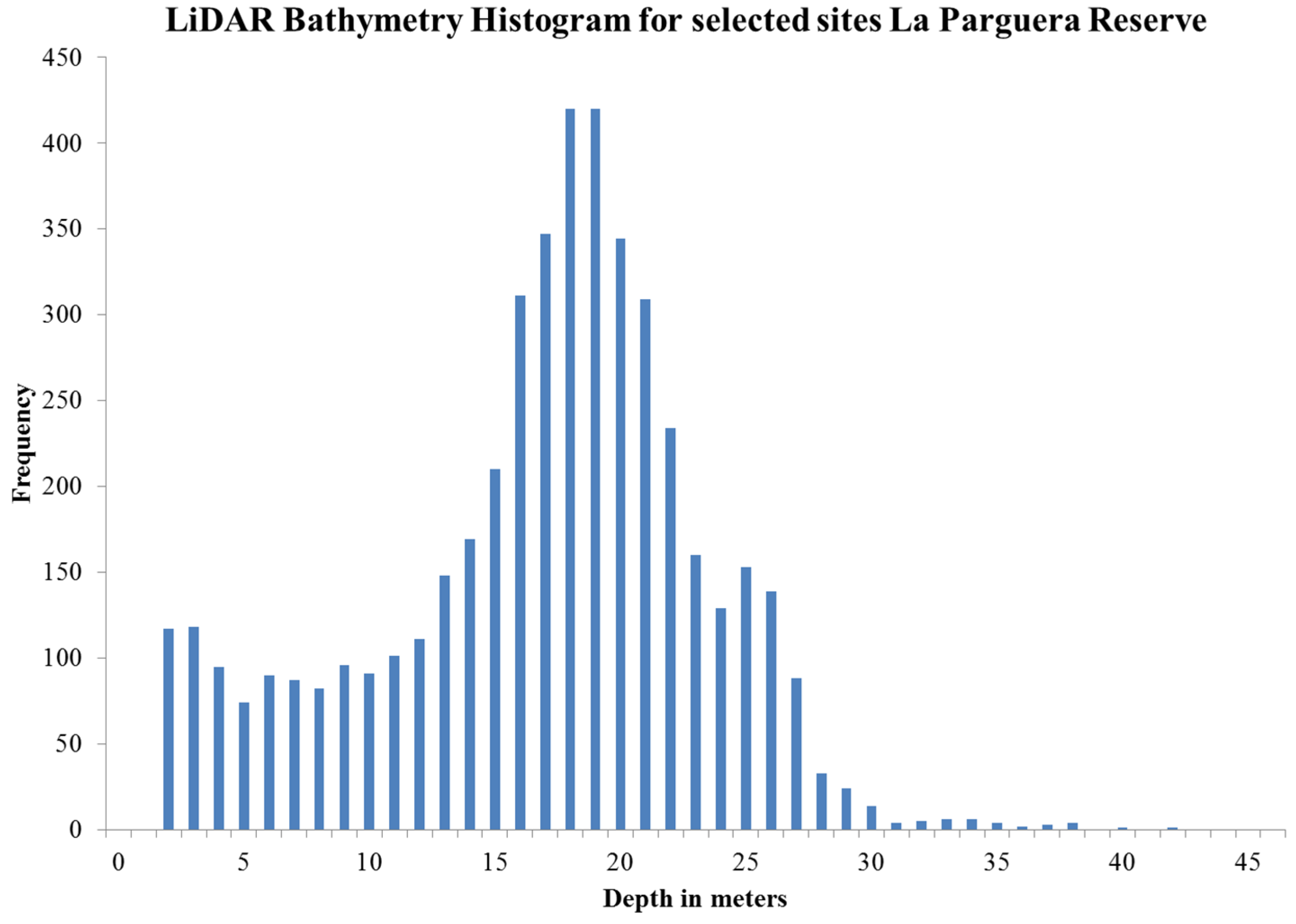
LiDAR bathymetry data for the study area ranged from 0 to 46 m. The inner shelf area can be distinguished by its complex physiography of submerged patch and emergent reefs, inshore cays, and mud and seagrass plains and depths ranging from 0 to 20 m. The mid and outer shelf have a wider range of depths ranging from 10 to 47 m, with the deeper areas located in the southwest area of the reserve (>30 m) near the shelf edge. This area is characterized by extensive coral reef development, especially near the shelf edge, where depth of this habitat can range from approximately 12 to 35 m. The average depth is approximately 16 m for the selected areas (
Figure 5).
Figure 5.
LiDAR SHOALS depth frecuency histogram for the selected points in La Parguera Reserve.
Figure 5.
LiDAR SHOALS depth frecuency histogram for the selected points in La Parguera Reserve.
4.3. Simple Band Ratios
Different band ratios were developed to determine the best ratio to retrieve bathymetry from the WV2 image. The band selection was based in selecting bands in the blue/green region that provided the best water penetration for successful bathymetry retrieval. Based on this approach 3, 2 band ratios (B1/B2, B1/B3, B2/B3) from WV2 visible bands were selected for six depth ranges. The correlation coefficient was calculated to test the performance of band ratios for different atmospheric corrections and was also divided in six depth ranges to evaluate the influence of depth. (
Table 1)
Table 1.
The coefficient of determination (r2) for six depth ranges for the different atmospheric corrections. The performance of each band ratio on (B1/B2, B1/B3, B2/B3) was evaluated when compared with LiDAR bathymetry per pixel values.
Table 1.
The coefficient of determination (r2) for six depth ranges for the different atmospheric corrections. The performance of each band ratio on (B1/B2, B1/B3, B2/B3) was evaluated when compared with LiDAR bathymetry per pixel values.
| | No Atmospheric Correction | Dark Subtract | FLAASH | Cloud Shadow |
|---|
| Depth | Band Ratio | r2 | r2 | r2 | r2 |
|---|
| 25–35 m | B1/B2 | 0.061 | 0.146 | 0.000 | 0.073 |
| B1/B3 | 0.154 | 0.229 | 0.174 | 0.175 |
| B2/B3 | 0.037 | 0.121 | 0.063 | 0.054 |
| 20–30 m | B1/B2 | 0.015 | 0.096 | 0.008 | 0.020 |
| B1/B3 | 0.277 | 0.315 | 0.103 | 0.316 |
| B2/B3 | 0.239 | 0.318 | 0.145 | 0.265 |
| 15–25 m | B1/B2 | 0.031 | 0.099 | 0.002 | 0.033 |
| B1/B3 | 0.169 | 0.248 | 0.047 | 0.222 |
| B2/B3 | 0.212 | 0.272 | 0.076 | 0.276 |
| 10–20 m | B1/B2 | 0.042 | 0.052 | 0.008 | 0.044 |
| B1/B3 | 0.086 | 0.134 | 0.024 | 0.121 |
| B2/B3 | 0.100 | 0.141 | 0.026 | 0.156 |
| 5–15 m | B1/B2 | 0.132 | 0.188 | 0.044 | 0.161 |
| B1/B3 | 0.254 | 0.465 | 0.067 | 0.408 |
| B2/B3 | 0.289 | 0.425 | 0.063 | 0.524 |
| 0–10 m | B1/B2 | 0.098 | 0.097 | 0.035 | 0.182 |
| B1/B3 | 0.283 | 0.596 | 0.090 | 0.576 |
| B2/B3 | 0.350 | 0.359 | 0.095 | 0.723 |
The best overall correlation was by using B2/B3 with the CSA atmospheric correction for the depth range of 0–10 m (r2 = 0.72). The best performance for the image with no atmospheric correction was the band ratio B2/B3 for the 0–10 m depth (r2 = 0.35). For the dark subtract atmospheric correction the band ratio B1/B3 provided the best performance and was for the depth range of 0–10 m (r2 = 0.60). For the atmospheric correction FLAASH, the best performance for WV2 was the band ratio B1/B3 for the 25–35 m depth band (r2 = 0.17).
The band ratios were also evaluated including all sampled points and depth ranges and the performance for the no atmospheric correction was B1/B2 = 0.04, B1/B3 = 0.48, B2/B3 = 0.60; for dark subtract correction B1/B2 = 0.69, B1/B3 = 0.86, B2/B3 = 0.85; for the FLAASH atmospheric correction were B1/B2 = 0.29, B1/B3 = 0.45, B2/B3 = 0.46, and for the CSA atmospheric correction were B1/B2 = 0.64, B1/B3 = 0.86, B2/B3 = 0.88.
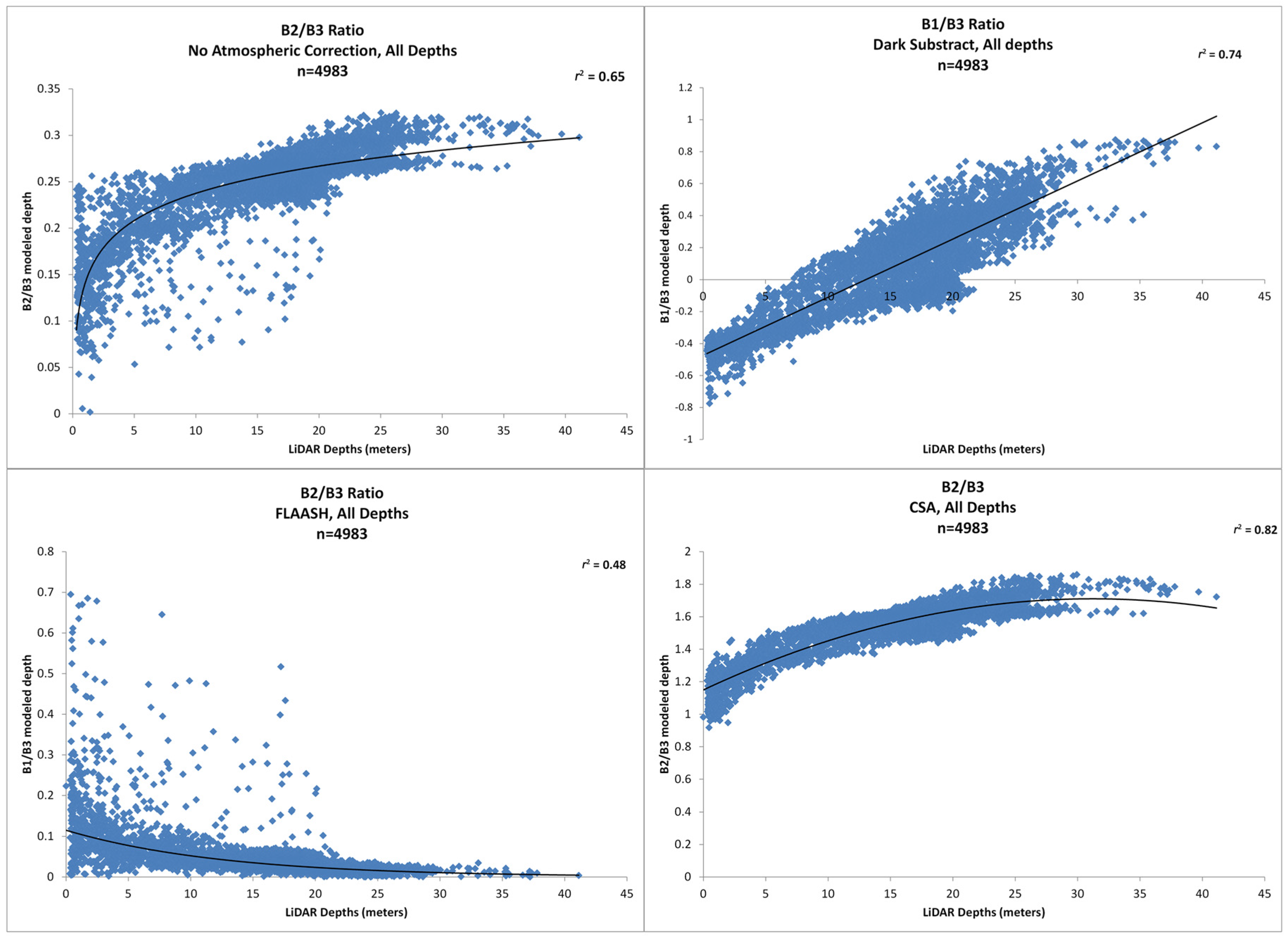
Based on the Pearson-product moment relationships of band ratios for different atmospheric corrections, we selected the best models to determine a best-fit equation for the relationship. For the band ratio with no atmospheric correction the equation of best fit was a second order polynomial (
r2 = 0.65), for the dark subtract atmospheric correction was a lineal equation (
r2 = 0.74), for the FLAASH atmospheric correction the best fit was an exponential equation (
r2 = 0.48), and for the CSA atmospheric correction the best fit was a second order polynomial (
r2 = 0.82) (
Figure 6).
Figure 6.
Coefficient of determination and best models to determine an equation of best fit for the relationship between the band ratios of WV2 image and LiDAR SHOALS data. The correlations presented are for no atmospheric correction (Top Left), the dark subtract atmospheric correction (Top Right), the FLAASH atmospheric correction (Bottom Left), and the CSA atmospheric correction (Bottom Right).
After the selection of the best band ratio and model for the relationship, a site validation was used to evaluate the model performance in retrieving depth for other locations within the WV2 image.
This model was applied to the image and analyzed for accuracy in depth estimation when compared with LiDAR depths. We also evaluated the influence of the atmospheric correction in the bathymetry retrievals.
4.4. WV2 Model Validation
The model from the B2/B3 ratio from CSA with a second order polynomial equation (
y = −0.0006
x2 + 0.0359
x + 1.1498) was applied to another location within the WV2 image (
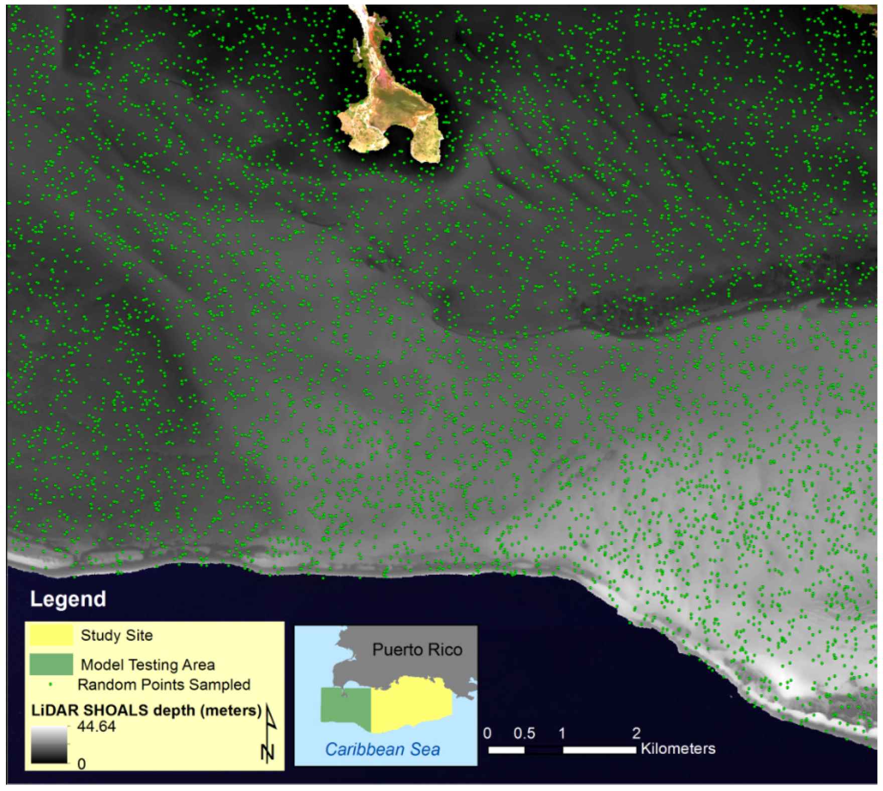
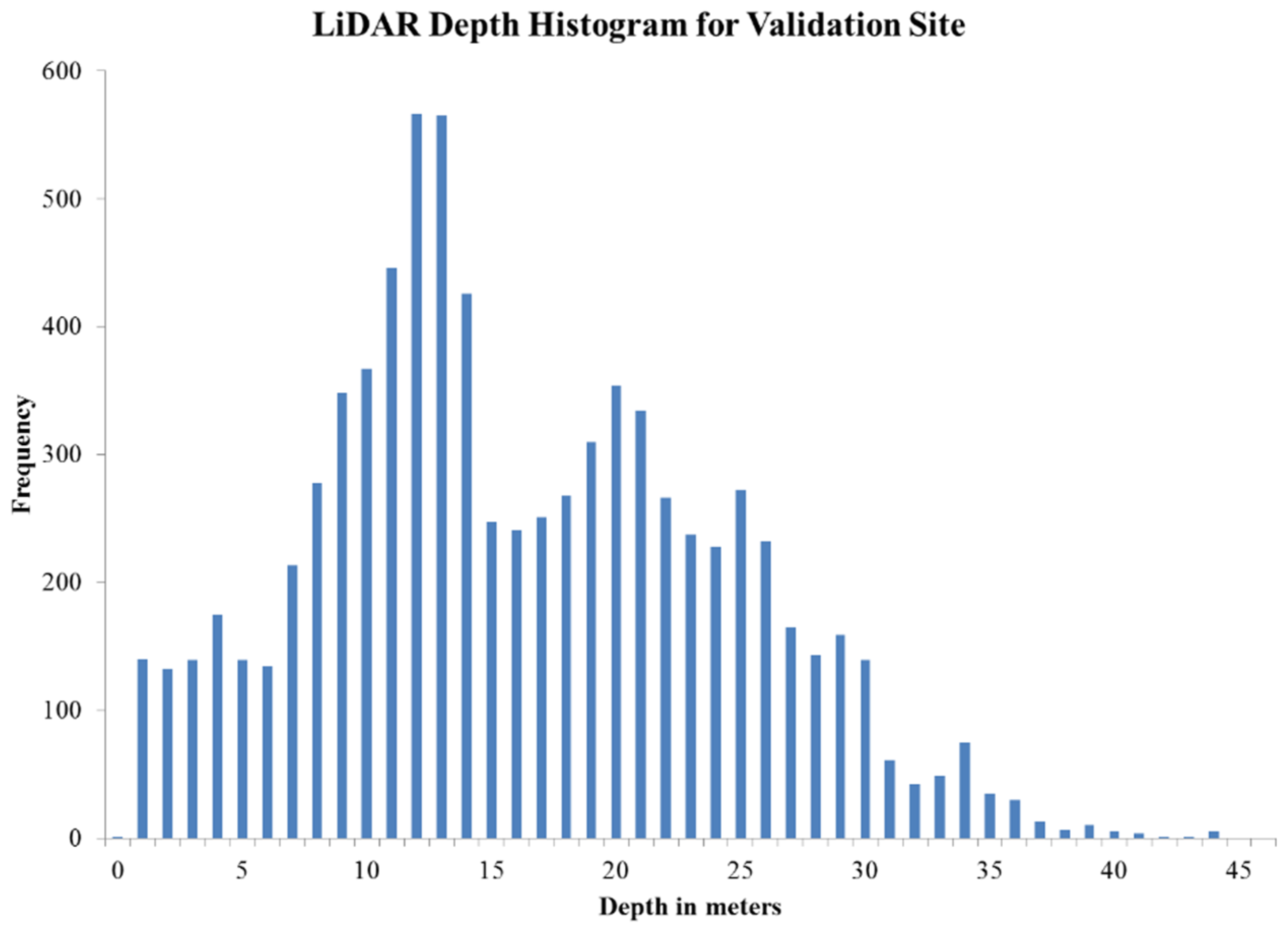
Figure 7) This model was applied to the image and analyzed for accuracy of the model in depth estimation when compared with LiDAR depths. The validation area shows an average depth of 15.7 m with a depth range from 1 to 43 m (
Figure 8).
Figure 7.
Validation site within the WV2 image off Southwestern Puerto Rico.
Figure 7.
Validation site within the WV2 image off Southwestern Puerto Rico.
Figure 8.
LiDAR SHOALS depth frecuency histogram for the selected points in the site validation area in Southwestern Puerto Rico.
Figure 8.
LiDAR SHOALS depth frecuency histogram for the selected points in the site validation area in Southwestern Puerto Rico.
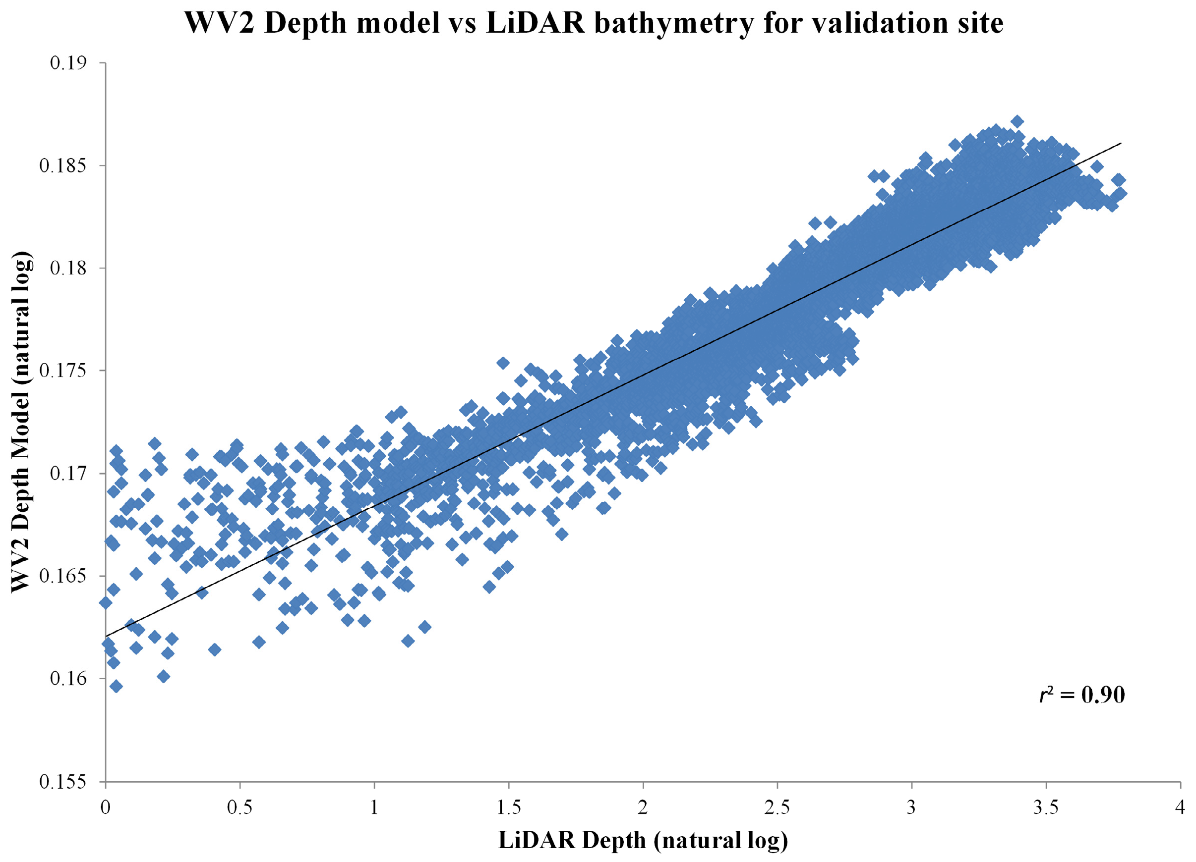
The values collected from WV2 Depth Model and LiDAR bathymetry were log transformed and then plotted to validate the model performance in estimating depth (
Figure 9). The coefficient of determination (
r2) was 0.90 for all the depth values sampled. The values were also analyzed to determine the model performance by depth range (
Table 2).
Figure 9.
Linearized (Ln) Relationship between values of the WV2 Depth Model and the LiDAR SHOALS depth (meters).
Figure 9.
Linearized (Ln) Relationship between values of the WV2 Depth Model and the LiDAR SHOALS depth (meters).
Table 2.
A coefficient of determination (r2), standard error, standard deviation and the Root Mean Square Error (RMSE) for six depth ranges for the WV2 depth model for validation. WV2 Depth Model vs. LiDAR SHOALS.
Table 2.
A coefficient of determination (r2), standard error, standard deviation and the Root Mean Square Error (RMSE) for six depth ranges for the WV2 depth model for validation. WV2 Depth Model vs. LiDAR SHOALS.
| Depth Range | r2 | St. Dev. (m) | N | Standard Error | RMSE |
|---|
| 1–10 m | 0.72 | 3.54 | 1921 | 1.58 | 1.26 |
| 5–15 m | 0.70 | 6.42 | 3591 | 2.16 | 1.47 |
| 10–20 m | 0.69 | 9.54 | 3672 | 2.47 | 1.57 |
| 15–25 m | 0.44 | 14.36 | 2760 | 2.80 | 1.67 |
| 20–30 m | 0.18 | 17.36 | 2180 | 3.00 | 1.73 |
| 25–35 m | 0.07 | 19.67 | 1101 | 3.16 | 1.78 |
| All depths | 0.90 | 10.54 | 8110 | 2.43 | 1.56 |
The WV2 depth model successfully retrieved depth values with an
r2 = 0.70 to a depth range of 20 m. Additionally, of the total values considered (
n = 8110), 69% of these were between the depth range of 1–20 m (
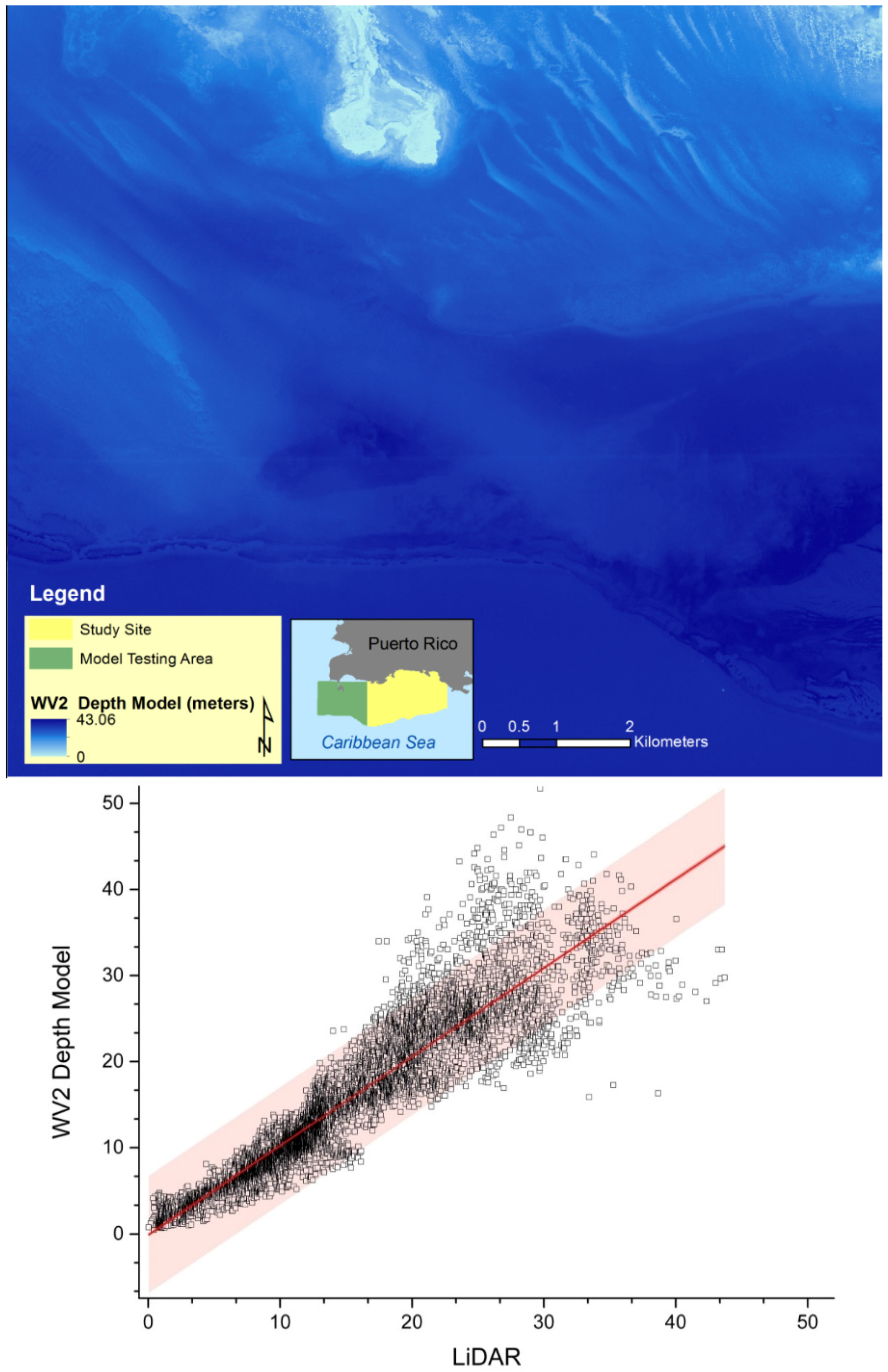
n = 5600). The aggregated RMSE for the validation values of the WV2 depth model was 1.56 m. These values of RMSE increase from 1.26 m for the 0–10 m depth range to 1.78 m for the 25–35 m depth range. A derived-bathymetry image was generated from the model used (
Figure 10).
Figure 10.
(Top) Depth estimation based on WV2 depth model for validation site within the WV2 image off southwestern Puerto Rico. (Bottom) Depth values (in meters) for WV2 depth model and LiDAR depths with 95% confidence and prediction bands. Note values dispersion after 20-m depth.
Figure 10.
(Top) Depth estimation based on WV2 depth model for validation site within the WV2 image off southwestern Puerto Rico. (Bottom) Depth values (in meters) for WV2 depth model and LiDAR depths with 95% confidence and prediction bands. Note values dispersion after 20-m depth.
5. Discussion
The water depth models tested here showed the importance of the atmospheric correction used in high-resolution multispectral image analysis. The data followed the results of Collin and Hench [
12] where the relation between modeled and actual depths varied as a function of the atmospheric correction used. This empirical model using regression-based modeling requires to take into account the local set of conditions of the study area and the atmospheric effects on the signal path length [
29]. Since the sensible depth is a function of the wavelength used and water clarity [
1], different band ratios were evaluated. The waters of La Parguera Reserve although considered oligotrophic, are susceptible to sediment resuspension, CDOM input from streams, and higher chlorophyll concentrations especially in the inner-shelf area [
30].
5.1. WV2 Depth Model
For the WV2, the cloud shadow atmospheric correction provided the best results (
r = 0.875) of all models tested including all the depth values and depth ranges that were analyzed. Both the cloud shadow and the dark subtract corrected values (
r = 0.772) show an improvement from the values using no atmospheric correction (
r = 0.592), confirming that the atmospheric correction is an essential pre-processing step in the image analysis process [
8]. As expected with bathymetry models from passive sensors [
31], the shallower values from the depth band of 0–10 m provide the best correlation between modeled and actual values (
Table 1). This correlation presented a gradual decrease with increasing depth, and for the depth range 25–35 m, these values were significantly reduced. However, for this maximum depth range the correlation was improved from 0.397 from the no atmospheric correction, to 0.479 and 0.418 for the dark subtract correction and cloud shadow corrections, respectively.
For the dark subtract the best model used the combination of the “coastal” band (425 nm) with the green band (B1/B3 = 0.863) for all depth values. The use of the “coastal” band in combination with the green band outperformed the traditional band combination that other high spatial resolution sensors provide (i.e., QuickBird, IKONOS) where the blue band is centered at 480 nm. For the cloud shadow atmospheric correction the best model used the combination of the blue and the green bands (B2/B3 = 0.823) for all depth values.
The coefficient of determination was obtained and an equation of “best fit” and applied to our depth models. The model with the cloud shadow atmospheric correction provided the best performance (r2 = 0.823). For each of the depth ranges the r2 decreased with depth from the highest r2 = 0.732 at 0–10 m, 0.532 at 5–15 m, to 0.162 at 10–20 m, suggesting that the model performance is reduced for values deeper than 15 m deep, as expected.
For the band ratio with no atmospheric correction the equation of best fit was a linear (
r2 = 0.638), and for the FLAASH atmospheric correction the best fit was an exponential equation (
r2 = 0.481) (
Figure 5). The scatterplot for the FLAASH atmospheric correction show the values dispersed from the exponential model for all depths up to the 23 m depth band. A present limitation of the FLAASH model for atmospheric correction is that WV2 imagery does not include bands for determining water vapor and aerosols [
12]. Our results showed that the analytical atmospheric correction (FLAASH) provided poorer results than no atmospheric correction and the dark subtract correction.
5.2. WV2 Depth Model Validation
The WV2 depth model successfully retrieved depth values with an r2 = 0.90 for all depth ranges, and of 0.70 to a depth range of 20 m at the validation site. The derived bathymetry map is important since it provides good depth estimates to 20 m, which represents 75% of the total depth range of the study area.
Other researchers have reported various depth ranges and values using band ratios but these were limited to shallow areas with very high water clarity [
4,
8], which contrast significantly with our study area that consist of variable bathymetry, heterogeneous bottom composition and geographic extent. Additionally, the random point’s selection for the model was not limited to a specific depth range (
i.e., 15 m) or a geographic location (
i.e., near-shore). By including this near-shore areas with higher turbidity and deeper areas the model represents more realistic conditions and the limitations of the image derived bathymetry using the WV2 image. Similar to our results, other researchers have used a site-specific model and obtained good results to 20 m [
10,
11], and to 30 m [
12].
The WV2 depth model was adjusted using LiDAR SHOALS bathymetry data an assumed that the LiDAR values were obtained with minimal error. According to Costa [
15], the pixels with the largest depth differences estimated by the LiDAR bathymetry for our site (that were greater than the maximum allowable vertical error) occurred primarily along the shelf edge in water deeper than 35 m. Although approximately only 25% of our study area exceeds the 20-m depth range, this limitation in the accuracy of the bathymetry from the LiDAR image in deeper areas, combined with the significant water attenuation effects of the passive signal, limits the retrieval of more accurate depths in these areas.
6. Conclusions
This study presents the first broad scale (168 km
2) bathymetry map for La Parguera Reserve derived from a passive sensor over a broad depth range and to the limits of detection of WV-2 data in these waters, which is also related to the bottom albedo signal. It also provided a comprehensive evaluation of the different atmospheric corrections and the influence in the water depth retrievals. This study also confirms that atmospheric correction methods should be applied to WV2 imagery prior to the development of bathymetric maps in order to increase the accuracy of the final product [
1,
12,
32]. Additionally, the selection of the atmospheric correction method is extremely important in the performance of the depth model, even for simple blue/green ratios, and can be determinant based on the final product that will be developed from the imagery (
i.e., benthic habitat map, depth retrievals).
In our case the best model was the one that use the Cloud Shadow Approach with a Band 2/Band 3 combination for the study area of La Parguera Reserve. This atmospheric correction proved successful even when it was modified due to cloud absence in the scene. Also, the use of simple band ratios provided the first high-resolution bathymetry map for La Parguera Reserve from passive sensors. The dark subtract correction provided the second best results and proved to be an excellent first approach for the correction of the atmospheric influence. The temporal difference in bathymetry of five years between the LiDAR bathymetry (2006) and the WV2 image (2011) were assumed minimal for the study area at this spatial scale. Additionally, the water quality conditions allowed for successful retrieval of bathymetry using passive sensor, which may not be the case in very high turbid waters. Using these methods, high-resolution bathymetry can be obtained from passive multispectral sensors with minimum processing while utilizing the information contained in the imagery.


