Article

Dynamically Scaled Model Experiment of a Mooring Cable

1
Division of Marine Technology, Department of Shipping and Marine Technology, Chalmers, Göteborg SE-412 96, Sweden
2
Department of Hydraulics, School of Civil Engineering, Chalmers, Göteborg SE-412 96, Sweden
*
Author to whom correspondence should be addressed.
These authors contributed equally to this work.
J. Mar. Sci. Eng. 2016, 4(1), 5; https://doi.org/10.3390/jmse4010005
Submission received: 23 November 2015 / Revised: 28 December 2015 / Accepted: 15 January 2016 / Published: 25 January 2016
(This article belongs to the Special Issue Ocean Wave Energy Conversion)

Abstract

:
The dynamic response of mooring cables for marine structures is scale-dependent, and perfect dynamic similitude between full-scale prototypes and small-scale physical model tests is difficult to achieve. The best possible scaling is here sought by means of a specific set of dimensionless parameters, and the model accuracy is also evaluated by two alternative sets of dimensionless parameters. A special feature of the presented experiment is that a chain was scaled to have correct propagation celerity for longitudinal elastic waves, thus providing perfect geometrical and dynamic scaling in vacuum, which is unique. The scaling error due to incorrect Reynolds number seemed to be of minor importance. The 33 m experimental chain could then be considered a scaled 76 mm stud chain with the length 1240 m, i.e., at the length scale of 1:37.6. Due to the correct elastic scale, the physical model was able to reproduce the effect of snatch loads giving rise to tensional shock waves propagating along the cable. The results from the experiment were used to validate the newly developed cable-dynamics code, MooDy, which utilises a discontinuous Galerkin FEM formulation. The validation of MooDy proved to be successful for the presented experiments. The experimental data is made available here for validation of other numerical codes by publishing digitised time series of two of the experiments.

Graphical Abstract

1. Introduction

The dynamic response of mooring cables for marine structures is scale-dependent, and perfect dynamic similitude between full-scale prototypes and small-scale physical model tests is difficult to achieve. In many physical experiments, the cable stiffness has been modelled by fitting springs at the ends of segments—e.g., at the anchor or at submerged buoys—which then produces correct scaling of the cable stiffness in a quasi-static sense only [1,2,3,4,5]. In the modelling of deep-sea moored floating systems it is often necessary to mimic the static reaction of catenary mooring systems with such springs, because of the limited depth or limited horizontal extension of the model tank [6]. For the wind turbine SPAR in [7] the truncation has been accomplished with some success by changing the lowest parts of the mooring cables to a heavy cable. The mooring system of the wave-energy device in [8] was truncated by removing those parts of the mooring cables constantly resting on the sea bed. For the purpose of validating numerical codes of the cable dynamics, however, it is preferable to compare against physical models, where the dynamic behaviour of the tension force is also related to that of the full-scale prototype. Such models are said to have dynamic similitude.
The purpose of this paper is to present results from a dynamic experiment with a chain submerged in water and make the experimental data available for validation of a numerical codes. The 33 m experimental chain can be considered a scaled 76 mm stud chain with a length of 1240 m, i.e., at a length scale of 1:37.6. A special feature of the experiment is that the chain was scaled to have correct propagation celerity for longitudinal elastic waves, thus providing a perfect geometrical and dynamic scaling in vacuum, which is unique. The physical model was then able to reproduce the effect of snatch loads giving rise to tensional shock waves propagating along the cable. The similarity in water was, however, not perfect due to viscous effects. The scaling is thoroughly discussed and the presented modelling approach using a specific set of dimensionless groups is compared to the scaling approaches used by [9] and [2], who formed two other sets of dimensionless groups. In [10] another two sets of dimensionless groups were used.
The upper end point of the chain was excited in a circular orbit with various radii and periods. The force in the upper end was recorded. Two typical examples of registered forces as function of time have now been meticulously digitized, and for thirty combinations of radii and periods the maximum forces in the cable during the excitation are given in tables and graphs. Due to the well-defined experimental conditions and the unique dynamic similitude, the results of the experiments are very well suited for validation of numerical simulation codes for cable dynamics, and may as such be of interest to a broader community. The experimental results have already been used for validation of dynamic cable codes by [11,12,13]. The data presented here will make validation both easier and more stringent.
Before the 1970s the calculations of the oscillatory motion of large, moored floating structures were done without considering the dynamic response of the mooring cables and presumed a linearized stiffness reaction from their mooring systems, post-processed by a nonlinear static estimation of the maximum tension in the mooring cables. This is the so-called quasi-static mooring procedure [14]. When the offshore industry progressed into deeper waters and made increasing use of floating platforms, first for drilling and service tasks later for floating production, it became apparent that dynamic mooring cable analysis was needed for survival design. For the analysis of the motion of smaller floating ships [15] and, for example, a one-point moored buoy [16] a dynamic analysis of the whole system is much more important.
Lately, it has been pointed out that, especially for wave energy converters the mooring design must be an integral part of the wave power systems design. The mooring design can significantly influence the efficiency of the wave power extraction and the operation and maintenance [17]. Also, there are significant engineering challenges to the positioning of such converters in exposed, shallow-water regimes [18]. The mooring system must ensure the desired station-keeping properties with a minimum footprint and without affecting the power output of the device in an excessively negative way. Cable damping due to the interaction with the sea-bed, internal friction and viscous drag forces is in this context an important feature of the mooring design [9,19]. In numerical cable modelling, the drag coefficient of the cable is therefore a critical parameter for the dynamic response, but is often chosen with some uncertainty [20]. For survival cases of wave energy converters, the design wave is often large compared to the water depth, leading to relatively large mooring excitations. This increases the risk of cable slack, often followed by a highly transient snatch load of large amplitude when the cable is retightened [21]. Traces of such snatch-loads are clearly visible in the experimental results presented in this paper.
In Section 2, the scaling is discussed; in Section 3, the experimental set-up is specified and the experimental results are given; and in Section 4, comparisons are presented with simulation results from a newly developed, very accurate cable-dynamics code, MooDy, using a discontinuous Galerkin FEM formulation [12]. The almost perfect agreement between experiments and numerical simulation is a strong indication that both the physical model and the numerical model are of high quality. Using the present input in other codes should give a similarly good fit.

2. Dynamic Similitude

The equation of motion of a mooring cable without bending stiffness is given in Section 2.1. In Section 2.2 the equation of motion is reduced to a non-dimensional form to investigate the conditions for dynamic similitude in a model test. The result is exploited in Section 3 to construct a suitable experimental model.

2.1. Governing Equations

The equation of motion of a mooring cable has been provided by many authors. See for instance [22,23,24,25]. The formulation used here is inspired by the one formulated in tangent and normal coordinates in [25] but is formulated in global coordinates and was developed in [26] by the last author. It takes elongation into account in the linear momentum conservation as well as for the external hydrodynamic forces, which is not common for all formulations. It neglects, however, contraction. Later in [4] a similar formulation was used but with a lower order strain formulation. In the present formulation the friction between the cable and the sea bottom is assumed to be small and is therefore neglected. However, the equation of motion, Equation (1), given below, is valid for a cable sliding on the sea bottom without friction. This equation of motion will be the starting point for our discussion of similarity.
γ o x _ ¨ + C 4 ( 1 + ε ) x _ ¨ C 4 ( 1 + ε ) ( x _ ¨ · x _ ) x _ s o ( K ε ˜ x _ ) f _ = 0
In Equation (1), x = [x1 x2 x3]T is the position vector of the cable in a Cartesian coordinate system with the origin at the anchor point, the coordinate x1 directed vertically upwards perpendicular to the sea bottom and the coordinate x2 horizontally in the plane of the resting cable. The sea bottom is assumed to be flat, horizontal and parallel to the mean sea surface. See Figure 1. The terms in Equation (1) represent forces per length unit of unstretched cable. The first term is the mass inertia force on the cable. The second and third terms are forces perpendicular to the cable that arise due to the acceleration in the water. The forth term is the reaction force of the cable. Finally, the fifth term, f, represents the external forces. The hydrodynamic forces due to the acceleration in the water (second and third term) and the drag forces contained in the external forces (fifth term) due to the relative velocity in the water are derived from the common Morison equation, and follows ideas in [27].
Figure 1. A mooring chain in a rectangular Cartesian coordinate system.
Jmse 04 00005 g001
In Equation (1), x = [x1 x2 x3]T is the position vector of the cable and γo the cable mass per length unit of unstretched cable:
C 4 = C M N π d o 2 4 ρ w
C M N : coefficient of added mass; do: characteristic diameter of the cable; ε, ε ˜ : longitudinal strains of the cable; K: the cable stiffness; t: time; so: curvilinear coordinate from the origin along the unstretched cable to a material point P; x ˙ = t ; x ¨ = 2 t 2 ; x = s o .
The fifth term is the resultant of three forces:
f _ = f _ ( 1 ) + f _ ( 2 ) + f _ ( 3 )
Weight and buoyancy, f _ ( 1 )
f _ ( 1 ) = [ 0 , g γ b , 0 ]
g γ b = ρ c ρ w ρ c g γ o   weight in water per unit unstretched length
ρ c cable density; ρ w water density.
Drag force tangential to the cable, f _ ( 2 )
f _ ( 2 ) = C 2 | v _ · x _ | ( v _ · x _ ) x _ 1 ( 1 + ε ) 2
v _ = v _ c x _ ˙   relative water velocity
v _ c : free stream velocity
C2 = (1/2) CDT do ρw
CDT tangential drag force coefficient
Drag force normal to the cable, f _ ( 3 )
f _ ( 3 ) = C 3 ( v _ · v _ 1 ( 1 + ε ) 2 ( v _ · x _ ) 2 ) ½ ( ( v _ ( v _ · x _ ) ) x _ 1 ( 1 + ε ) 2 ) ( 1 + ε )
C3= (1/2) CDN do ρw
CDN normal drag force coefficient
In the expressions above two estimates of the longitudinal strains, ε and ε ˜ , are used, which are equal to first order and related by
( 1 + ε ) 2 = ( 1 + 2 ε ˜ )
ε ˜ = ( 1 2 ) ( x _ · x _ 1 )

2.2. Dimensionless Variables and Dynamic Similarity

Similarity conditions can be formulated from the equation of motion. The conditions are dynamically similar if the model and prototype can be described by the same equation of motion and boundary conditions except for some constant factor. Rules for dynamic similitude of cables have been formulated by, e.g., [1] and similar results are obtained from the following analysis. While [1] formulated the equation of motion in tangential and normal coordinates, we here use the formulation in Section 2.1. We assume that the equations are applicable in both model and prototype.
The following dimensionless coordinates are introduced:
s = so/L
τ = t/T
y = x/L
Here L is a characteristic length and T a characteristic time. The characteristic length can, e.g., be chosen as the total unstretched length of the cable and the characteristic time as some characteristic time period of the motion of the upper end of the cable.
From Equations (13) the derivatives of x become
x _ ˙ = y _ τ L T
x ¨ _ = 2 y _ τ 2 L T 2
x _ = y _ s
We introduce a dimensionless free-stream velocity, v _ c * , via
v _ c = v _ c * L T
Substitution of Equations (14) and (15) into the relative velocity Equation (7) then yields
v _ = ( v _ c * y _ t ) L T
and a dimensional relative velocity v _ * via
v _ = v _ * L T
where
v _ * = ( v _ c * y _ t )
Alternatively the free-stream velocity can be a function of x _ = x _ ( s o , t )
v _ c = F _ ( x _ )
and a dimensionless function F _ * = F _ * ( y _ )
v _ c = F _ * ( y _ ) L T
Equivalently to (2.16), the free-stream velocity can now be written
v _ = ( F _ * ( y _ ) y _ t ) L T
and a dimensionless relative velocity as
v _ * = F _ * ( y _ ) y _ t
Introducing Equations (14) and (21) into the equation of motion Equation (1) we now realize that this can be formulated with y as the independent variable. To avoid long tedious expressions we will, however, use Equation (17) instead of Equation (21). Below we also assume constant material properties along the cable length. After division by γoL/T2 we then get the following dimensionless equation:
2 y _ τ 2 + α 1 ( 1 + ε ) 2 y _ τ 2 α 1 ( 1 + ε ) ( 2 y _ τ 2 · y _ s ) y _ s α 2 s ( ε ˜ y _ s ) f _ * = 0
where
f _ * = f _ * ( 1 ) + f _ * ( 2 ) + f _ * ( 3 )
and
f _ * ( 1 ) = [ 0 , α 3 , 0 ] T
f _ * ( 2 ) = α 4 | v _ * · y _ s | ( v _ * · y _ s ) y _ s 1 ( 1 + ε ) 2
f _ * ( 3 ) = α 5 ( v _ * · v _ * 1 ( 1 + ε ) 2 ( v _ * · y _ s ) 2 ) ½ ( v _ * ( v _ * · y _ s ) · y _ s 1 ( 1 + ε ) 2 ) ( 1 + ε )
where
ε ˜ = ( 1 2 ) ( y _ s · y _ s 1 )
The relationships between the strains are as before ( 1 + ε ) 2 = ( 1 + 2 ε ˜ ) (Equation (11))
In the equations above, α1, α2, α3, α4, and α5 are dimensionless parameters:
α 1 = C 4 γ o
α 2 = K T 2 γ o L 2
α 3 = γ b g T 2 γ o L
α 4 = C 2 L γ o
α 5 = C 3 L γ o
We introduce an expression for the cable mass per unit unstretched length:
γ o = C v π d o 2 4 ρ c
where Cv is a volume coefficient. For a wire rope or a circular solid steel rod, Cv = 1. Then, with the help of Equations (2), (8), (10), (29), and (30), we can interpret the dimensionless parameters α 1 to α 5 as
α 1 = C M N C v ρ w ρ c = a d d e d   m a s s c a b l e   m a s s
α 2 = c 2 T 2 L 2 = ( w a v e   c e l e r i t y c h a r a c t e r i s t i c   v e l o c i t y ) 2 = 1 M 2
α 3 = ( 1 ρ w ρ c ) g T 2 L = w e i g h t i n e r t i a = ( 1 ρ w ρ c ) g ( c h a r a c t e r i s t i c   l e n g t h ) ( c h a r a c t e r i s t i c   v e l o c i t y ) 2 = ( 1 ρ w ρ c ) 1 F r 2
α 4 = 2 π C D T L C v d o ρ w ρ c
α 5 = 2 π C D N L C v d o ρ w ρ c
where c = K / γ o is the propagation celerity of longitudinal elastic waves, for short, denoted wave celerity, M = ( L / T ) / c a Mach number and F r = ( L / T ) / ( g L ) a Froude number. The introduction of these special Mach and Froude numbers is inspired by [1].
We can see that α 2 is the inverted Mach number squared, and that for the Mach number = 1, a tensional disturbance will travel all along the characteristic length of the cable in just one characteristic period. For larger Mach numbers and larger characteristic velocities (L/T) or, equivalently, smaller α 2 , the longitudinal tensional distribution will become increasingly less uniform. We may also note that α 3 is the inverted Froude number squared multiplied by the relative density difference between cable and water. The parameter α 3 governs the swinging, inelastic gravity waves.
Complete dynamic similitude requires that all the five non-dimensional numbers α are equal between the model and prototype.

2.3. Scale Factors

To achieve dynamic similarity, the corresponding five parameters, α and the dimensionless current must all be equal in model and prototype. We assume first that the densities, ρw, and ρc, and the earth acceleration, g, are the same in the model and prototype, which is very common. Equation (31a) then indicates that the ratio CMN/Cv shall be equal in model and prototype. We then introduce the length scale λ:
L m L p = λ
where the index m and p denote the cable length in, respectively, the model and prototype. The time scale can subsequently be derived from (2.31c) assuming α3 to be equal:
T m T p = λ
Similarly the scale of wave celerity is given by (2.31b), (2.32) and (2.33):
c m c p = λ
An additional scale β is now introduced [1], the ratio between model and prototype diameters:
d o m d o p = β
This scale may provide the freedom to choose the model diameter independently of the length scale.
The ratio between the stiffness in the model and prototype can then be deduced from Equations (30) and (34) using the fact that the wave celerity is c = K / γ o   .
K m K p = c m 2 c p 2 γ o m γ o p = C v m C v p λ β 2 = φ λ β 2
where we introduced the volume coefficient scale, φ = C v m / C v p .
As the strain must be the same in the model and prototype, the scale of the tension force in the cable must be the same as the scale of stiffness.
F m F p = φ λ β 2
Equations (31e), (32) and (35) give the scale of normal drag-force coefficients
C D N m C D N p = β φ λ
The same scale is valid for the tangential drag-force coefficients.
An important parameter for assessing the added-mass and drag-force coefficients is the Reynolds number, Re = v d o / ν , where v and do are characteristic values of, respectively, the relative velocity and the cable diameter, and ν is the kinematic viscosity. The scale of the relative velocity is
v m v p = λ
Assuming the same fluid (viscosity) in model and prototype, the relation between the Reynolds numbers would be
Re m Re p = β λ
The Reynolds number should ideally be the same in the model and prototype, which is not possible in this case with the same fluid as β = d o m / d o p λ . The correct Reynolds number was achieved in [28] for two modelled cable structures using highly viscous test fluids and specially fabricated filaments. These models concerned quasi-steady towing and dynamic experiments for anchor-last deployments at the length scales 1:1000 and 1:2000. However, in the present case we must achieve equality of α 3 containing a Froude scaling, and in a complete model with a floating platform we must necessarily achieve equality of the free-surface Froude number. In our case with a submerged cable generating almost no waves it suffices to achieve equality of α 3 . The scales Equations (32), (33), (35), (37), (38), (39), and (40) are those given by [1] setting Cv = 1 above. The stiffness scale Equation (2.36) was introduced by [13]. In [1] it is proposed that Equations (38) and (40) can be utilised with experimental data of the drag coefficients as functions of the Reynolds number to get drag-force similarity. In [1], this is shown for a cable with a circular cross section using different scales, λ and β. Similarity of both tangential and transverse drag forces normally cannot be achieved.
In Section 3 we will use the results above to construct a suitable physical dynamic model of a cable.

3. Physical Experiments

In the experiments a decoration chain was used. It was suspended in a water basin such that one end was partly resting on the concrete floor of the basin. The other, upper end was attached to a rotating sheave above the water surface. The attachment point on the sheave was set at various radii to its centre of rotation and the electrical motor could produce various rotational speeds, so that the upper attachment point was excited in circular paths at various radii and periodicity. The force in the chain close to its upper attachment point was measured. The choice of chain and other parameters are accounted for in Section 3.1 and Section 3.2. Experimental equipment and procedures are described in Section 3.4 and Section 3.5. As key results, the measured maximum forces during the excitation cycles after reaching stationary oscillations are given in Section 3.6.

3.1. Choice of Chain

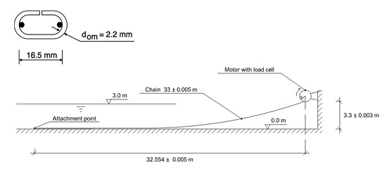
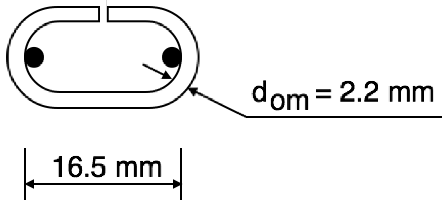
We chose a lacquered decoration chain with “open” links. “Open” means that the link loops were not welded after bending. The shape of the links is pictured in Figure 2.
Figure 2. The shape and dimensions of the chain links.
Jmse 04 00005 g002
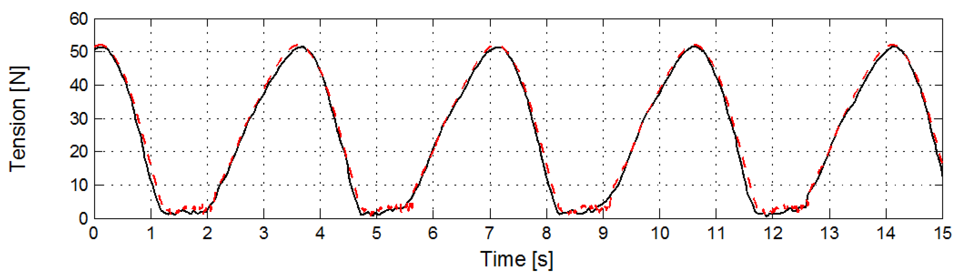
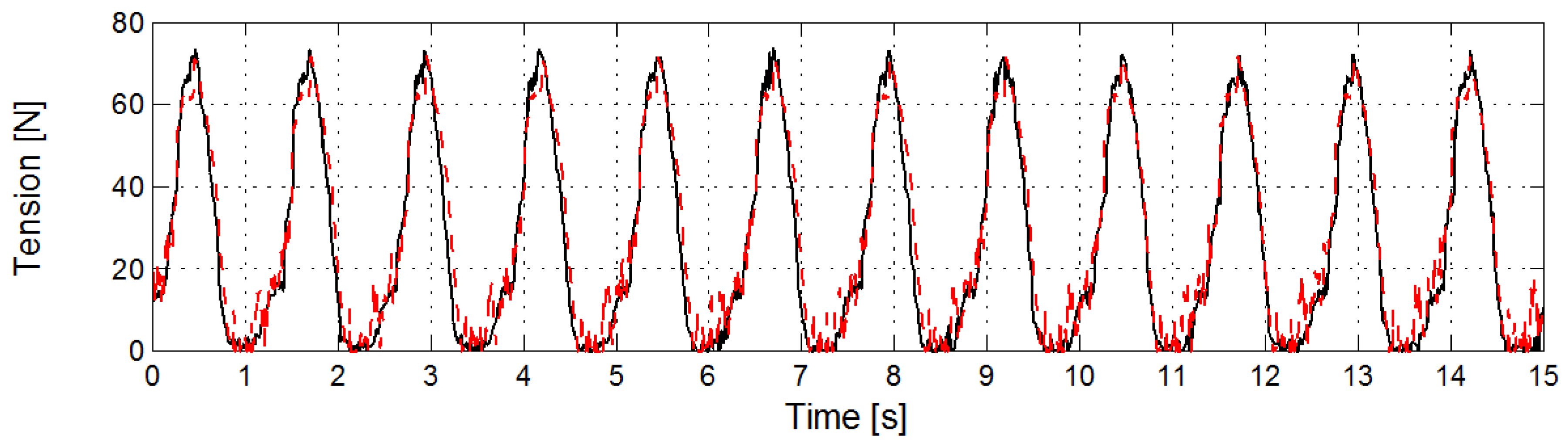
A few lengths of chain were tested in a tensile tester to get the relation between strain and pulling force. The relation was almost linear for a pulling force lower than 200 N. The stiffness of the chain was measured at Km = 10,000 ± 500 N, which is a low value caused by the links being open. Again, the index m denotes model values and the index p prototype values.
The mass of the chain per unit length was measured to γom = 0.0818 ± 0.0005 kg/m by weighing a long length of the chain. The longitudinal wave speed was then calculated as c m = K m / γ o m 350   m / s . The density was assumed to be 7800 kg/m3, neglecting the thin lacquer.
The link diameter of the model chain was dom = 2.2 mm. A prototype chain in a mooring system can have a link diameter of dop = 76 mm. Such a chain has the stiffness of Km = 5.8 × 10⁸ N [29] and the mass γop = 126.5 kg/m [29,30] but the same density as the model chain, because both are made from steel. The longitudinal wave speed can then be calculated as c p = K p / γ p m 2143   m / s .
The two chains can be compared with respect to dynamic similarity. Through Equation (34) the length scale can be calculated as
λ = ( c m c p ) 2 = ( 350 2143 ) 2 = 0.02663
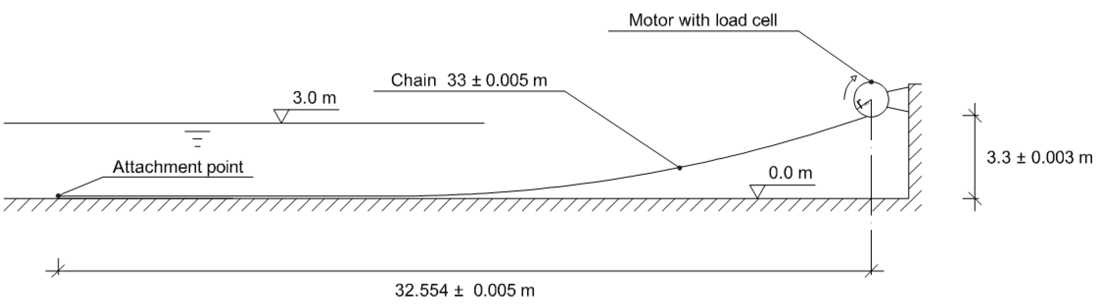
In the physical experiment the chain length was chosen to be Lm = 33 ± 0.005 m for practical reasons and to get a somewhat taut cable. The vertical span from the concrete floor to the mean elevation of the upper attachment point was 3.3 m. The chain length also included a shackle and a force probe in the upper end with the length 0.159 m and a shackle in the other, lower end with a length of 0.026 m. These are neglected in the numerical simulations in Section 4. With λ = 0.027 and Lm = 33 m the length of the prototype chain would become Lp 1240 m.
These two chains thus fulfil the necessary conditions to be dynamically similar for oscillations in vacuum, i.e., without hydrodynamic forces, and the dimensionless parameters α 2 and α 3 are equal between the model and prototype. To assess the hydrodynamic scaling we revert to Equations (31a) and (38).
According to Equations (31a) α1 should be the same in the model as in the prototype
α 1 m α 1 p = C M N m C v m ρ w ρ c C M N p C v p ρ w ρ c = C M N m C v p C M N p C v m = C M N m C M N p 1 φ = 1
The volume coefficient of the model chain was calculated to be Cvm 2.76 and that of the prototype chain to be Cvp 3.58. Then, the volume coefficient scale is φ = Cvm/Cpm 0.74. See Equation (36). The ratio between the added mass coefficients in the model and the prototype can then be solved from Equation (42):
C M N m C M N p = φ = 0.771
The scale β = dom/dop = 2.2/76 = 0.029 and λ = 0.027 inserted in Equation (38), based on α 5 being equal, gives the ratio between the normal drag coefficients in the model and the prototype as:
C D N m C D N p = β φ λ = 0.029   · 0.74 0.033 = 0.839
To judge whether the hydrodynamic forces are similar, relevant data from the coefficients are needed. However, we can note that the added-mass and the drag coefficients shall, at least, have the same order of magnitude in model and prototype.
The parameters α 1 , α 4 and α 5 contain the normal added-mass coefficient C M N , the tangential drag coefficient C D T and the normal drag coefficient C D N , which all are functions of the Reynolds number, R e m a x = u m a x d o / ν , and the Keulegan-Carpenter number, K C = u m a x T / d o . At the upper end the transverse maximum velocity of the cable during a cycle is u m a x = 2 π r / T , where r is the radius of excitation. Then we can write R e m a x = 2 π r d o / ( T ν ) and K C = 2 π r / d o .
In the present experiments 300 < R e m a x < 2200 and 210 < K C < 570 . In the prototype 6.3 · 10 4 < R e m a x < 4.7 · 10 5 and 230 < K C < 620 . Thus one may conclude that the KC number is almost equal in the model as in the prototype and also well above 50, a value where the dependence of the added mass coefficient on the Keulegan-Carpenter number is flattening out for circular cylinders. See for instance an experimental graph by Sarpkaya (Figure 3.18 in [31]). The authors have found no qualified information on added mass for chains in the literature, but a qualified guess is that the added mass coefficient of the prototype chain is somewhat larger than that of the model chain, which gives a better agreement for Equation (43). A first guess would be to set the added mass coefficient equal to the volume coefficient. Furthermore, as the density of steel is 7.8 times greater than the density of water, the exact value of the added-mass coefficient may not be very important for this case, but may be more significant for lighter synthetic ropes.
If we assume almost stationary flow at the present very high KC numbers, we can expect a rather constant drag coefficient C D 1 1.2 for 500 < R e < 5 · 10 5 . At the upper limit it sharply drops to 0.3 and then gradually rises to 0.6 at 6 ×   10 6 . See for instance a graph based on experiments with circular rods by Schlichting (Figure 3.1b in [31]) or Figure 12 in [32]). Thus C D 1 in both the model and the prototype near the upper end of the cable; C D N m / C D N p 1 instead of 0.84 according to Equation (44). However, the transverse velocity at the mid span of the hanging part of this relatively taut cable may be around 10 times greater than the excitation velocity at the upper end. The drag coefficient would then be expected to drop to 0.5 in the prototype for the mid span. This would give C D N m / C D N p 2 i.e., which does not agree as well with Equation (44). However, the discussion is strictly valid for circular cylinders only. In DnV-OS-E301 [33] the normal drag coefficient is recommended to have a value of 2.6 for a stud chain and 2.5 for a studless chain, using the material diameter as the diameter in the drag expression. The present decoration chain is, however, less compact than the prototype stud chain, which is why the drag coefficient may be a little lower.

3.2. Choice of Other Conditions

The model chain was suspended so that it partly rested on the concrete floor of the basin and was fixed to a lead weight at the far end. The configuration is shown in Figure 3. The upper end was attached to a rotating sheave with its centre 0.3 m above the water surface. This implies that the submerged length of chain varies somewhat during an excitation period.
Figure 3. Experimental set-up.
Jmse 04 00005 g003
The attachment point on the sheave was set at various radii, rm, to its centre of rotation and the electrical motor at various rotational speeds to produce various periods, Tm. Table 1 and Table 2 show the radii of excitation and the period times respectively, for both model and prototype scale.
Table 1. Radii rm (m) Circular upper-end excitation in model and prototype scale.
Model0.0750.1000.1250.1500.200
Prototype2.823.754.695.637.51
Table 2. Periods, Tp (s) Period time of circular upper-end excitation.
Periods, Tp (s)1.251.52.02.53.03.5
Periods, Tp (s)7.79.212.315.318.421.5

3.3. Alternative Dimensional Analyses

There are many possibilities for grouping non-dimensional parameters. For instance, in [10] two approaches using either the displacement amplitude or the velocity amplitude as the forcing function are formulated, resulting in two sets of nine dimensionless groups, two of which are different. Here, however, we will compare our modelling using the dimensionless groups presented in [9] and [2].
A complete list of the data of the model and the prototype are given in Table 3.
Table 3. Input data for the parameters in Table 4, Table 5 and Table 6.
QuantityModelPrototype
L33m1240mLength of cable
V3.3m124.0mVertical span
do0.0022m0.076mMaterial diameter
de0.00365m0.144mEquivalent solid-rod diameter (reference diameter)
w = ( 1 ρ w / ρ c ) g γ o 0.699N/m1078N/mWeight in water
Ts22.68N1.314 × 106NStatic tension
K10kN5.8 × 105kNStiffness
umax0.135–1.0m/s0.825–6.16m/sExcitation speed
ν10−6m2/s10−6m2/sKinematic viscosity
ρ c 7800kg/m37800kg/m3Cable density
ρ w 1000kg/m31024kg/m3Water density
r0.075–0.2m2.82–7.51mDiameter of motion
ψ0.455rad0.454radAngle between motion and the horizontal
C v 2.76-3.58-Volume coefficient
Webster [9] formulates a non-dimensional tension in a cable as a function of 12 non-dimensional parameters. See Table 4. These include the running time over the period of excitation, the moment of inertia in bending over the cross-sectional area squared, two parameters containing CD and Cm—essentially depending on the Reynolds number—and one containing the steady current drag over the weight of the mooring line. In our physical model there is no bending stiffness, there is no current and the drag and added-mass parameters may be combined into a Reynolds number. This leaves us with nine parameters. These are checked below for the presented model. Papazoglou et al. [2] and Mavrakos et al. [3] also present nine non-dimensional parameters for similitude, but not in the same combinations.
Table 4. The nondimensional parameters (groups) used by Webster [9] and relevant for this problem with Webster’s explanations of their physical meanings. Notations as in the present article.
Parameter
t/Tis the time relative to the period of the sinusoidal excitation. If a steady state is achieved, the state of the mooring line repeats for each unit increment in this parameter; This parameter scales with the square root of the length scale and is not listed explicitly below in Table 5 and Table 6;
L/Vis the ratio of the mooring line length to the vertical span and is commonly called the “scope” of the mooring line;
Ts/(wV)is the ratio of the static pretension of the mooring line to the weight in water of a length of mooring line equal to the vertical span. This parameter, together with the scope, governs the geometry of the mooring line when no motions are imposed;
r/Vis the ratio of the amplitude of motion to the water depth;
C D C v is the ratio of the hydrodynamic, cross-flow drag forces acting on the real mooring line to those which would act on the reference mooring line if exposed to the same flow situation;
C m C v is the ratio of the added mass loads to those which would act on the reference mooring line exposed to the same flow situation;
T 2 π g V is the ratio of the period of the excitation to the period of a pendulum of length V;
ρ w / ρ c is the ratio of the water mass density to the mass density of the mooring line material. This parameter measures the relative importance of the hydrodynamic loads to the internal mechanical loads;
K/wLis the inverse of the strain at the top of the cable resulting from suspending the mooring line vertically in water of unrestricted depth. This parameter measures the relative “stiffness” of the mooring line;
do/Vis the ratio of the diameter of the reference mooring line to the vertical span. Since almost all mooring lines are exceptionally thin compared to the vertical span, this parameter approaches zero.
Table 5. Nondimensional parameters according to [9] calculated for the present experimental data with the notations used in the present article.
ParameterModelPrototypeRatio Prototype/Model
1L/V10101
2Ts/(wV)1.0171.0181.00
3r/V0.023–0.0610.023–0.0611.00
4 C D C v CDm∙1.66CDp∙1.951.14 ( C D p / C D m )
5 C m C v Cmm∙2.76Cmp∙3.821.30 ( C m p / C m m )
6 T 2 π g V 0.343–0.9600.343–0.9601.00
7 ρ w / ρ c 0.1280.1311.02
8K/wL4354351.00
9do/V0.67 × 10−30.61 × 10−30.92
Table 6. Non-dimensional parameters according to [2] calculated for the present experimental data with the notations used in the present article.
ParameterModelPrototypeRatio Prototype/Model
1L/V10101
2do/L67 × 10−661 × 10−60.92
3wL/Ts1.0181.0161.00
4Remax = umaxdo300–22006.27 × 104–4.7 × 105212
5 ρ c / ρ w 7.807.620.98
6K/Ts4414421.00
7r/do34.1–90.937.1–98.81.09
8 ω 2 L 2 / ( T s / ( ρ c π d e 2 / 4 ) ) 12.7–99.212.7–99.51.00
9ψ0.4550.4541.00
The present model fulfils most of Webster’s parameters except the ones containing the coefficients of drag and added mass and the diameter over vertical-span ratio. See Table 5. The prototype over model ratio for Parameter 4 is 1.14 ( C D p / C D m ) and the ratio ( C D p / C D m ) may be between 0.5 and 1 referring to the discussion in Section 3.1. Then, 1.14 ( C D p / C D m ) would be in the range of 0.6 and 1.1, which may be considered reasonably correct. Parameter 5 would give the ratio 1.4 using the ratio for recommended added mass coefficients ( C mp / C mm ) = 2.6 / 2.5 . This is not completely satisfactory, but as said before, for a steel cable the steel mass dominates the inertia. Parameter 9 gives a prototype over model ratio of 0.92 because the diameter over vertical-span ratio d/V simply depends on the difference in steel material diameter which is a result of modelling compromises and this is of minor importance.
The present model also fulfils most of the parameters of [2]. See Table 6. The modelling error in Parameters 2 and 7 is caused by the different material diameters and scale β. Using the equivalent homogeneous rod diameter de instead of the material diameter do in Parameters 2 and 7, we would get prototype over model ratios of 1.05 and 0.96, respectively. As discussed above, the Reynolds number, Parameter 4, cannot be the same in the model and prototype. The modelling error in Section 5 is simply caused by the fact that we had fresh water in the model and assumed sea water in the prototype. As for Parameter 8, [2] does not discuss its physical significance, but again we may encounter a modelling error. If we use the diameter do instead of de the prototype over model ratio becomes 0.77.
We can conclude that the presented dynamic experiment with a chain submerged in water can be considered as a model of a 1240 m long 76 mm stud chain at a length scale of 1:37.6. As the chain was also scaled to have correct propagation celerity for longitudinal elastic waves, it provided a perfect geometrical and dynamic scaling in vacuum. In [1] it was pointed out that this is the most difficult scale to achieve, but here we have stated it is possible to accomplish this. The similarity in water was not perfect mainly due to viscous effects as the comparisons of non-dimensional parameters confirm. The main modelling error arises from the impossibility of achieving Reynolds number equality, but if the Reynolds number is high enough, the drag and added mass coefficients could be considered equal in model and prototype.

3.4. Experimental Equipment

The experiments were run in the manoeuvring basin at SSPA, Göteborg. At the short edge of the basin a rig with a speed-controlled electrical motor was erected. The chain was attached by a ball-bearing axis to a sheave on the axis of the motor at various distances from its centre. See Figure 4. The chain was hung parallel to the long side of the basin half a metre from this side. It was fixed at its far lower end by an anchor consisting of two lead weights. The force in the upper end of the chain was measured with a force probe (Bofors KK10). The force measurements were recorded on paper charts which now have been digitised. Please note that the digitisation process cannot properly recreate the high-frequency oscillations appearing at slack conditions. The high-frequency amplitudes are correctly captured from the charts but the number of oscillations might be underestimated. The peak loads and non-slack conditions are, however, well captured in the digitisation procedure.
Figure 4. The experimental rig with electrical motor, sheave, chain and force probe.
Jmse 04 00005 g004

3.5. Experimental Procedure

The radius of the excitation motion was set between the various fixed positions by moving a screw between predrilled and threaded holes. Thereafter the period of rotation was adjusted by controlling the speed of the motor. The periphery velocity was, however, affected a little by the fact that the sheave ran slower when the chain was pulled in than when it was let out. The deviation was judged to be negligibly small but was not measured. The time period was however correct. The force in the upper end point was recorded for a time long enough to reach stationary oscillatory conditions. For each radius a set of experiments with different periods were conducted. Before each set the force probe was calibrated. In total 30 experiments were performed and the mean maximum force was extracted from the time series. The reading error was estimated to be ±5% including the error of the force probe calibration.

3.6. Experimental Results

Two examples of recorded upper end force are shown in Figure 5 and Figure 6, from one long period test with Tm = 3.50 s, and one shorter period test with Tm = 1.25 s. In Figure 5 the tension response is slightly asymmetric, with a mild slope during the up-stroke and a sharper drop in the down-stroke. During approximately 1 s of the cycle the cable has virtually no stiffness as the major part is slack. When tension is regained, the response is still smooth because of the relatively long period oscillation. The same effects can be seen for the tension force record of the shorter period time in Figure 6, but here the re-tensioned cable gives rise to clearly visible transients in the tension force. This results in both a double peak appearance and a step-like behaviour of the tension force history during the upstroke motion.
In Table 7 the mean of the measured maximum upper-end tensions for each combination of period and radius in the experiments are listed. These are digitised from [13].
Figure 5. Recorded upper-end force Fm (N) for the period Tm =3.50 s and radius rm = 0.2 m. (Digitised from [13]).
Jmse 04 00005 g005
Figure 6. Recorded upper-end force Fm (N) for the period Tm =1.25 s and radius rm = 0.2 m. (Digitised from [13]).
Jmse 04 00005 g006
Table 7. Measured mean of maximum upper-end tension (N). (Digitised from [13]).
Period (s)Radius (m)
0.0750.10.1250.150.2
1.2542.546.854.160.470.3
1.5041.045.351.559.068.0
2.0036.039.547.554.162.3
2.5031.135.442.549.057.3
3.0029.533.139.345.854.0
3.5027.831.537.542.550.1

4. Simulated Tension

While [13] carried out simulations with the Modex code using standard finite elements [34], we here include simulation results from a newly developed cable dynamics code, MooDy [12], using discontinuous Galerkin elements to capture snap and snatch tensions. The MooDy cable model takes the bilinear stiffness of a chain into account with zero stiffness for compressive deformation. It includes a Morison formulation for the hydrodynamic loads as described in Section 2, Coulomb friction for the sliding on the bottom and a bilinear bottom stiffness for the vertical contact force with the bottom. In Table 8 the input model data is listed. One may note that the normal drag coefficient is the same as that recommended in DnV-OS-E301 for studless chains. The added mass coefficient was set to 3.8, which may be a little too high as the volume coefficient is only 2.8. This was investigated in [13] and it was found that the added mass could as well be set to 0 for the present cases. In the MooDy cable model the instantaneous submergence of the chain was taken into account.
Table 8. The input model data.
QuantityMeasureUnit
Water density1000kg/m3ρwm
Water depth3mThe coefficients of added mass and drag are as default set to zero above the water surface
Bottom:
Friction0.3-The friction coefficient is increasing linearly to the given value up to the sliding speed and 0.01 m/s
Coordinate0mVertical coordinate is x1 = 0 m at bottom and points upwards
Elastic modulus3 × 109PaFor x1 < 0 m but 0 Pa for x1 ≥ 0 m
Damping factor1-For x1 < 0 m but 0 for x1 ≥ 0 m
Cable:
Unstretched length33mLm
Horizontal span32.554mFrom anchor point to centre of sheave
Vertical span3.3mFrom bottom to centre of sheave
Density7800kg/m3ρc
Stiffness10000NKm
Mass per length unit0.0818kg/mγom
Steel diameter2.2mmdom
Normal drag coefficient2.5-Applied on the steel diameter dom
Tangential drag coefficient0.5-Applied on the steel diameter dom
Added mass coefficient3.8-Applied on the material area γom/ ρc
For comparison, the recorded and simulated upper-end forces in the model Fm (N) for the excitation radius rm = 0.2 m for the period Tm =3.50 s are drawn in Figure 7 and for Tm =1.25 s in Figure 8. Overall, the simulations match very well with the measured data, suggesting that all important dynamic effects are correctly accounted for in the numerical model. Some numerical oscillations are seen in the slack region of Figure 8. These are artefacts of the numerical settings used in MooDy (10 elements of polynomial order 7) and the ill-posed nature of the dynamic problem of cables under negative strain with negligible bending stiffness [35]. The results shown in Figure 7 and Figure 8 are unfiltered.
In Figure 9 the simulated maximum upper-end tensions of all combinations of (rm, Tm) are plotted as a function of measured maximum tension. The agreement is shown to be very good, with a correlation coefficient of R2 = 0.98 compared to full agreement.
Figure 7. Recorded (solid black) and simulated (dashed red) upper-end force Fm (N) for the period Tm =3.50 s and radius rm = 0.2 m.
Jmse 04 00005 g007
Figure 8. Recorded (solid black) and simulated (dashed red) upper-end force Fm (N) for the period Tm =1.25 s and radius rm = 0.2 m.
Jmse 04 00005 g008
Figure 9. Simulated versus measured maximum upper-end force Fmax (N) for various excitation periods Tm (s) and radii rm (m).
Jmse 04 00005 g009

5. Conclusions

The dynamic response of mooring cables for marine structures is scale dependent, and perfect dynamic similitude between full-scale prototypes and small-scale physical model tests is difficult to achieve. A notable feature of the experiment presented is that the chain was scaled to have correct propagation celerity for longitudinal elastic waves, thus providing perfect geometrical and dynamic scaling in vacuum, which is unique. The scaling error due to an incorrect Reynolds number seems to be of minor importance. The 33 m experimental chain can then be considered a scaled 76 mm stud chain with a length of 1240 m, i.e., a length scale of 1:37.6. The physical model was able to reproduce the effect of snatch loads giving rise to tensional shock waves propagating along the cable.
The results from the experiment were compared to results from the newly developed, very accurate cable-dynamics code, MooDy, which utilises a discontinuous Galerkin FEM formulation. The almost perfect fit of upper-end force in the time domain and a goodness of fit r2 = 0.98 of linear regression between simulated and measured force maxima are both strong indications that the physical model and the numerical model are of high quality. The comparison was made using the data of the physical model and thus involved no scaling errors, only the usual experimental inaccuracies, which are judged to be small. Using the present input in other codes should give a similarly good fit. The experimental data is herein made available for validation of other numerical codes through publishing digitised time series of upper-end force from two of the experiments.

Supplementary Materials

Supplementary File 1

Acknowledgments

The experiments were sponsored by the National Swedish Board of Technical Development (STU). Access to the SSPA manoeuvring tank was granted without charge, which was greatly appreciated. The development of the MooDy code was sponsored by Västra Götalandsregionen through the Ocean Energy Centre, as was the authoring of this article.

Author Contributions

Lars Bergdahl (L.B.) is the main author of the paper. L.B. carried out the discussion of similarity of drag and mass coefficients, the evaluation of alternative sets of non-dimensional parameters, and the comparison between the experimental results and the simulation results. Jan Lindahl planned and performed the experiments. He was also the main contributor to the discussion of modelling and similarity rules, which originally were used to design the experiments. Johannes Palm carried out the simulations in the MooDy code, Claes Eskilsson produced the digitisation of the experimental data, and together, J.P. and C.E. have been assisting L.B. in the assembly of the paper.

Conflicts of Interest

The authors declare no conflict of interest.

References

  1. Collier, M.L. Dynamic similarity scaling laws applied to cables. Engineering notes. J. Hydronautics 1972, 6, 111–114. [Google Scholar] [CrossRef]
  2. Papazoglou, V.J.; Mavrakos, S.A. Non-linear cable response and model testing in water. J. Sound Vib. 1990, 140, 103–115. [Google Scholar] [CrossRef]
  3. Mavrakos, S.A.; Papazoglou, V.J.; Triantafyllou, M.S.; Hatjigeorgiou, J. Deep water mooring dynamics. Mar. Struct. 1996, 9, 181–209. [Google Scholar] [CrossRef]
  4. Chen, X.; Zhang, J.; Johnson, P.; Irani, M. Dynamic analysis of mooring lines with inserted springs. Appl. Ocean Res. 2001, 23, 277–284. [Google Scholar] [CrossRef]
  5. Zhang, S.-X.; Tang, Y.-G.; Liu, X.-J. Experimental investigation of nonlinear dynamic tension in mooring lines. J. Mar. Sci. Technol. 2012, 17, 181–186. [Google Scholar] [CrossRef]
  6. Pronav, S.A. The specialist committee on deep water mooring. In Proceedings of the 22nd ITTC Conference, Seoul, Korea; Shanghai, China, 5–11 September 1999.
  7. Molins, C.; Trubat, P.; Gironella, X.; Campos, A. Design Optimization for a Truncated Catenary Mooring System for Scale Model Test. J. Mar. Sci. Eng. 2015, 3, 1362–1381. [Google Scholar] [CrossRef] [Green Version]
  8. Harnois, V.; Weller, S.D.; Johanning, L.; Thies, P.R.; le Boulluec, M.; le Roux, D.; Soulé, V.; Ohana, J. Numerical model validation for mooring systems: Method and application for wave energy converters. Renew. Energy 2015, 75, 869–887. [Google Scholar] [CrossRef] [Green Version]
  9. Webster, W.C. Mooring-induced damping. Ocean. Eng. 1995, 2, 571–591. [Google Scholar] [CrossRef]
  10. Cross, J.F. An Experimental Study of the Dynamics of Catenary Mooring Lines. Master’s Thesis, Memorial University of Newfoundland, St. John’s, NL, Canada, 1992. [Google Scholar]
  11. Gutiérrez, J.E.G. Desarrollo de Herramientas Software Para el Análisis de Aerogeneradores “Offshore” Sometidos a Cargas Acopladas de Viento y Oleaje. Ph.D. Thesis, Universidad Politécnica de Cartagena, Murcia, Spain, 2014. [Google Scholar]
  12. Palm, J.; Moura Paredes, G.; Eskilsson, C.; Taveira Pinto, F.; Bergdahl, L. Simulation of Mooring Cable Dynamics Using a Discontinuous Galerkin Method. In Proceedings of the V International Conference on Computational Methods in Marine Engineering, Hamburg, Germany, 29–31 May 2013.
  13. Lindahl, J. Modellförsök Med en Förankringskabel (Model Tests with a Mooring Cable, in Swedish); Report Series A:12; Department of Hydraulics, Chalmers University of Technology: Göteborg, Sweden, 1985. [Google Scholar]
  14. Furuholt, E. Mooring systems for offshore operations. Nor. Marit. Res. 1975, 3, 15–22. [Google Scholar]
  15. Wilson, B.W.; Garbaccio, D.H. Dynamics of ship anchor lines in waves and currents. J. Waterw. Harb. Div. 1969, 95, 449–466. [Google Scholar]
  16. Nath, J.W.; Felix, M.P. Dynamics of a single point mooring in deep water. J. Waterw. Harb. Div. 1970, 96, 815–833. [Google Scholar]
  17. Fitzgerald, J.; Bergdahl, L. Including moorings in the assessment of a generic offshore wave energy converter: A frequency domain approach. Mar. Struct. 2008, 21, 23–46. [Google Scholar] [CrossRef]
  18. Fitzgerald, J. Position Mooring of Wave Energy Converters. Ph.D. Thesis, Chalmers University of Technology, Göteborg, Sweden, 2009. [Google Scholar]
  19. Johanning, L.; Smith, G.; Wolfram, J. Measurements of static and dynamic mooring line damping and their importance for floating WEC devices. Ocean Eng. 2007, 34, 1918–1934. [Google Scholar] [CrossRef]
  20. Xu, Z.; Huang, S. Numerical investigation of mooring line damping and the drag coefficients of studless chain links. Mar. Sci. Appl. 2014, 13, 76–84. [Google Scholar] [CrossRef]
  21. Hann, M.; Greaves, D.; Raby, A. Snatch loading of a single taut moored floating wave energy converter due to focused wave groups. Ocean Eng. 2015, 96, 258–271. [Google Scholar] [CrossRef]
  22. Love, A.E.H. A Treatise on the Mathematical Theory of Elasticity; Cambridge at the University Press: Cambridge, UK, 1893. [Google Scholar]
  23. Routh, E.J. Dynamics of Systems of Rigid Bodies, 6th ed.; Dover Publications Inc.: Mineola, NY, USA, 1955. [Google Scholar]
  24. Szabo, I. Höhere Technische Mechanik 2 Auflage; Springer Berlin-Göttingen-Heidelberg: Berlin, Germany, 1958. [Google Scholar]
  25. Sander, G.; Geradin, M.; Nyssen, C.; Hogge, M. Accuracy versus computational efficiency in nonlinear dynamics. Comput. Methods Appl. Mech. Eng. 1979, 17–18, 315–430. [Google Scholar] [CrossRef]
  26. Lindahl, J.; Sjöberg, A. Dynamic Analysis of Mooring Cables. In Proceedings of the Second International Symposium on Ocean. Engineering and Ship Handling, Gothenburg, Sweden, 1–3 March 1983.
  27. Casarella, M.J.; Parsons, M. Cable systems under hydrodynamic loading. Mar. Technol. Soc. J. 1970, 4, 27–44. [Google Scholar]
  28. Parnell, L.A. Experimental Scale Modelling of Large Undersea Cable Structures. In Proceedings of the Oceans’80, Seattle, WA, USA, 8–9 September 1980.
  29. Ramnäs Bruk Product Catalogue, Visited online. Available online: http://ramnas.com/wp-content/uploads/2012/11/Ramnas-Technical-Broschure.pdf (accessed on 19 September 2015).
  30. Vicinay Cadenas. OFFSHORE MOORING CHAIN, DATA SHEET. Available online: http://www.vicinaycadenas.net/mooring-chain/offshore-mooring-chain.asp (accessed on 19 September 2015).
  31. Sarpkaya, T.; Isaacson, M. Mechanics of Wave Forces on Offshore Structures; Van Nostrand Reinhold Company: New York, NY, USA, 1981. [Google Scholar]
  32. Hoerner, S.F. Fluid-dynamic drag, 2nd ed.; Self-published book; June 1965. [Google Scholar]
  33. Det norske Veritas AS. Position Mooring; DNV-OS-E301; DNV: Høvik, Norway, 2013; Available online: https://rules.dnvgl.com/docs/pdf/DNV/codes/docs/2013-10/OS-E301.pdf (accessed on 20 January 2016).
  34. Lindahl, J.; Bergdahl, L. MODEX-MODIM, User’s Manual; Report Series B:49; Department of Hydraulics, Chalmers University of Technology: Göteborg, Sweden, 1987. [Google Scholar]
  35. Triantafyllou, M.S.; Howell, C.T. Dynamic response of cables under negative tension: An ill-posed problem. J. Sound Vib. 1994, 173, 433–447. [Google Scholar] [CrossRef]

