
Geovisualization of Mercury Contamination in Lake St. Clair Sediments


Abstract
:
1. Introduction
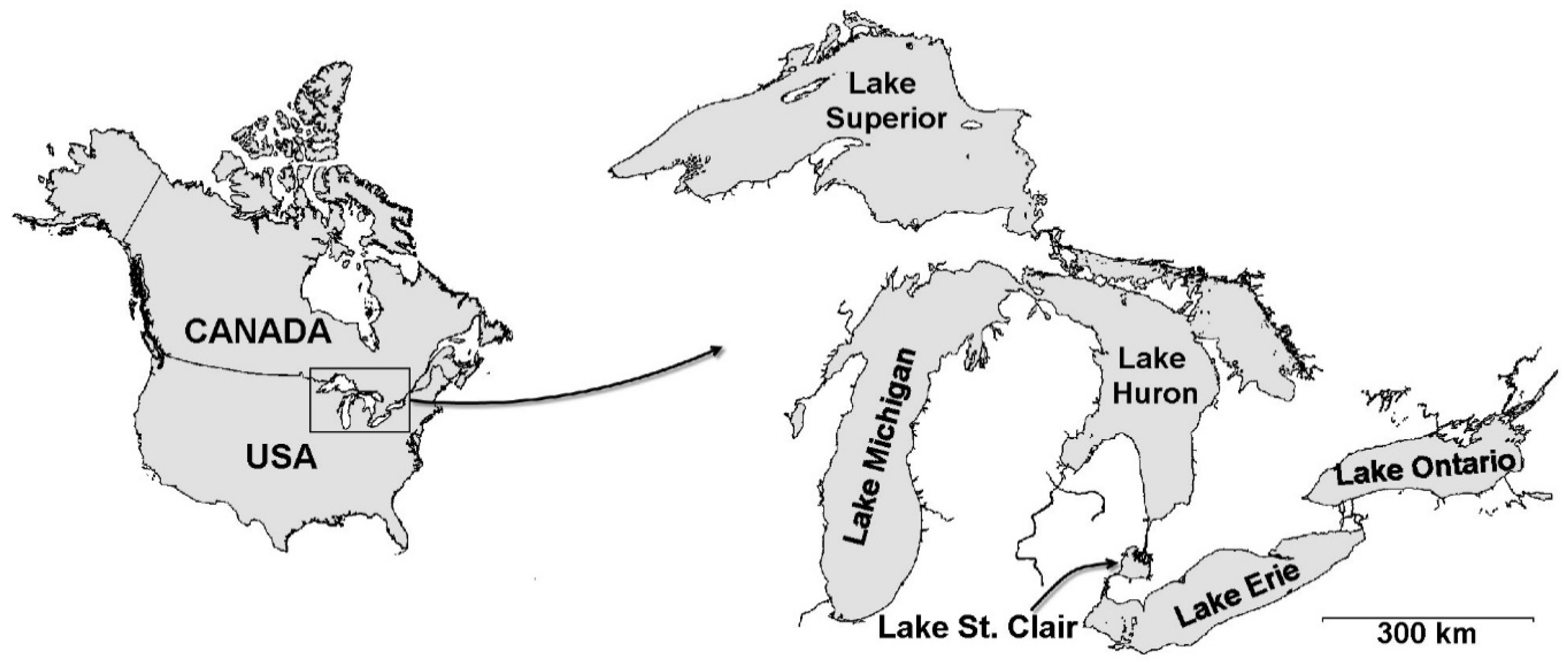
1.1. Study Area
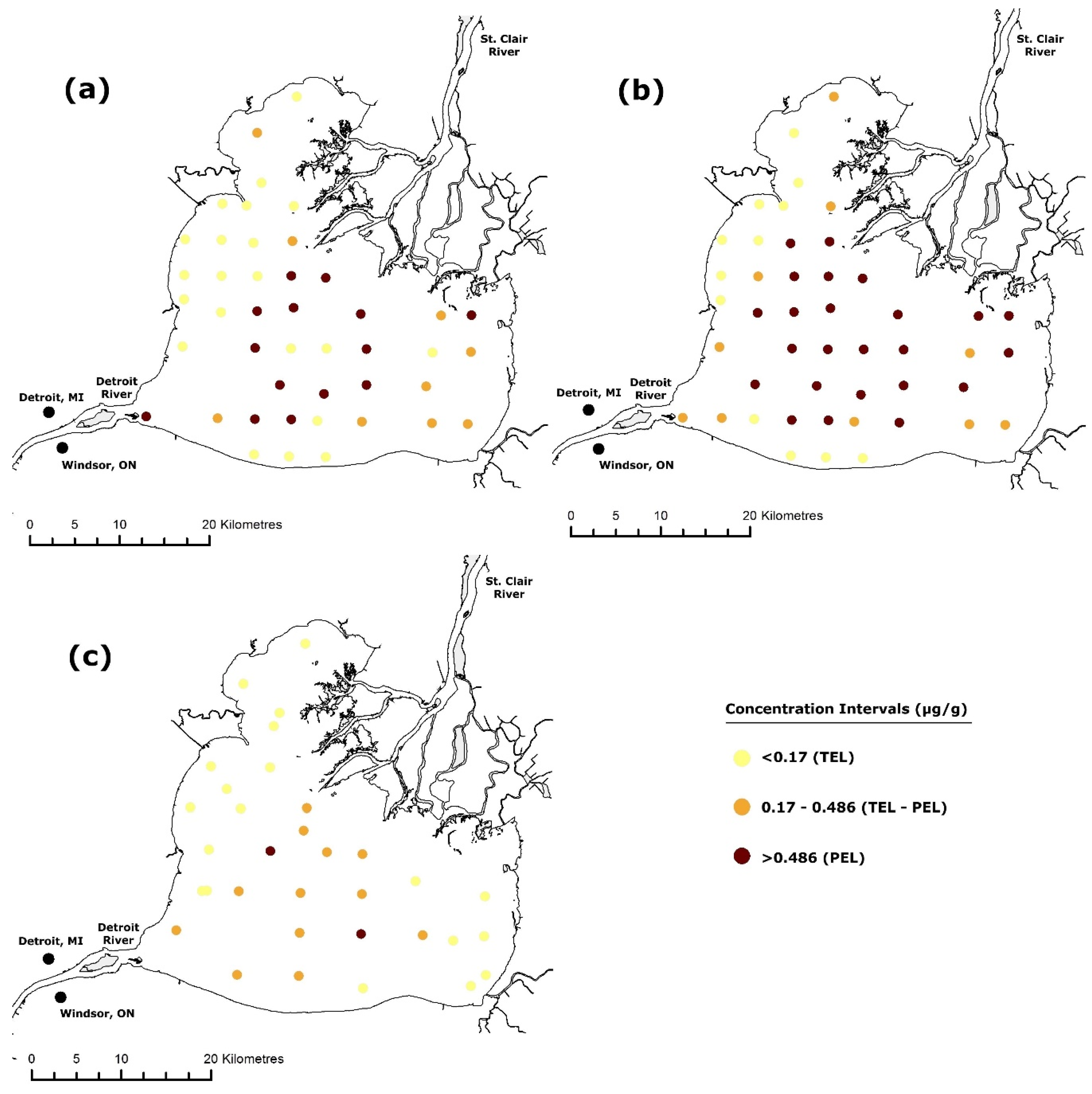
1.2. Data
2. Methodology
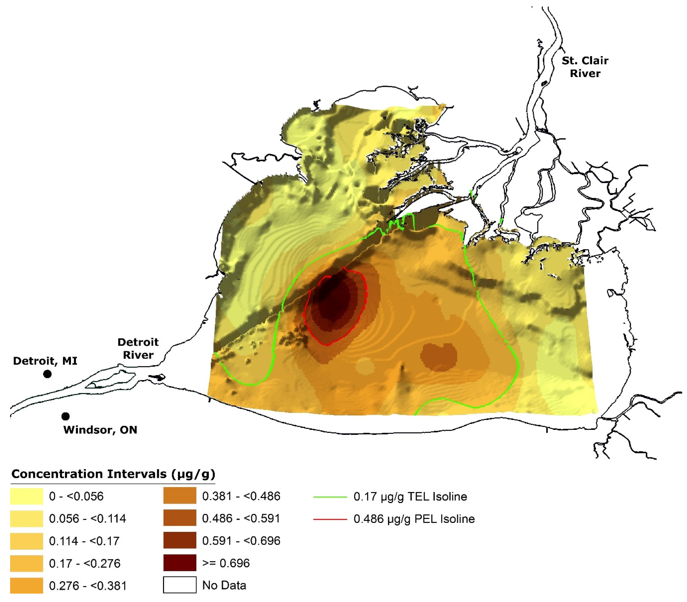
2.1. Interpolation
2.2. Visualization
3. Results and Discussion
Discussion
4. Conclusions
Author Contributions
Conflicts of Interest
References
- The Great Lakes Drainage Basin. Available online: https://www.ec.gc.ca/grandslacs-greatlakes/default.asp?lang=En&n=03B3F448 (accessed on 24 December 2015).
- Great Lakes Bathymetry. Available online: http://www.ngdc.noaa.gov/mgg/greatlakes/greatlakes.html (accessed on 24 December 2015).
- Wigle, O.; Vincent, J.; Wright, E. The Lake St. Clair Canadian Watershed Technical Report: An Examination of Current Conditions; Canadian Watershed Coordination Council: Strathroy, ON, Canada, 2008; pp. 1–83. [Google Scholar]
- Canadian Sediment Quality Guidelines for the Protection of Aquatic Life. Available online: http://ceqg-rcqe.ccme.ca/download/en/226 (accessed on 24 December 2015).
- Detroit River-Western Lake Erie Basin Indicator Project—Indicator: Mercury in Lake St. Clair Walleye. Available online: http://www.epa.gov/med/grosseile_site/indicators/hg-walleye.html (accessed on 24 December 2015).
- Ontario Ministry of the Environment. Guide to Eating Ontario Sport Fish; Queen’s Printer for Ontario: Toronto, ON, Canada, 2009; pp. 1–337. [Google Scholar]
- Canadian Council of Ministers of the Environment (CCME). Canadian Environmental Quality Guidelines; Canadian Council of Ministers of the Environment: Winnipeg, MB, Canada, 1999. [Google Scholar]
- Forsythe, K.W.; Marvin, C.H. Analyzing the spatial distribution of sediment contamination in the Lower Great Lakes. Water Qual. Res. J. Can. 2005, 40, 389–401. [Google Scholar]
- Forsythe, K.W.; Paudel, K.; Marvin, C.H. Geospatial analysis of zinc contamination in Lake Ontario sediments. J. Environ. Inform. 2010, 16, 1–10. [Google Scholar] [CrossRef]
- Gawedzki, A.; Forsythe, K.W. Assessing anthracene and arsenic contamination within Buffalo River sediments. Int. J. Ecol. 2012, 2012. [Google Scholar] [CrossRef]
- Jakubek, D.J.; Forsythe, K.W. A GIS-based kriging approach for assessing Lake Ontario sediment contamination. Gt. Lakes Geogr. 2004, 11, 1–14. [Google Scholar]
- Forsythe, K.W.; Irvine, K.N.; Atkinson, D.M.; Perelli, M.; Aversa, J.M.; Swales, S.J.; Gawedzki, A.; Jakubek, D.J. Assessing lead contamination in Buffalo River sediments. J. Environ. Inform. 2015, 26. [Google Scholar] [CrossRef]
- Gewurtz, S.B.; Shen, L.; Helm, P.A.; Waltho, J.; Reiner, E.J.; Painter, S.; Brindle, I.D.; Marvin, C.H. Spatial distribution of legacy contaminants in sediments of Lakes Huron and Superior. J. Gt. Lakes Res. 2008, 34, 153–168. [Google Scholar] [CrossRef]
- Gewurtz, S.B.; Helm, P.A.; Waltho, J.; Stern, G.A.; Reiner, E.J.; Painter, S.; Marvin, C.H. Spatial distributions and temporal trends in sediment contamination in Lake St. Clair. J. Gt. Lakes Res. 2007, 33, 668–685. [Google Scholar] [CrossRef]
- Gewurtz, S.B.; Bhavsar, S.P.; Jackson, D.A.; Fletcher, R.; Awad, E.; Moody, R.; Reiner, E.J. Temporal and spatial trends of organochlorines and mercury in fishes from the St. Clair River/Lake St. Clair corridor, Canada. J. Gt. Lakes Res. 2010, 36, 100–112. [Google Scholar] [CrossRef]
- Jia, J.; Thiessen, L.; Schachtchneider, J.; Waltho, J.; Marvin, C.H. Contaminant Trends in Suspended Sediments in the Detroit River-Lake St. Clair-St. Clair River Corridor, 2000 to 2004. Water Qual. Res. J. Can. 2010, 45, 69–80. [Google Scholar]
- ArcGIS; Version 10.2; Environmental Systems Research Institute (ESRI): Redlands, CA, USA, 2013.
- Resch, B.; Wohlfahrt, R.; Wosniok, C. Web-based 4D visualization of marine geo-data using WebGL. Cartogr. Geogr. Inf. Sci. 2014, 41, 235–247. [Google Scholar] [CrossRef]
- Alves, T.M.; Kokinou, E.; Zodiatis, G. A three-step model to assess shoreline and offshore susceptibility to oil spills: The South Aegean (Crete) as an analogue for confined marine basins. Mar. Pollut. Bull. 2014, 86, 443–457. [Google Scholar] [CrossRef] [PubMed]
- Smith, M.J.; Hillier, J.K.; Otto, J.-C.; Geilhausen, M. Geovisualization. In Treatise on Geomorphology; Shroder, J.F., Ed.; Academic Press: San Diego, CA, USA, 2013; Volume 3, pp. 299–325. [Google Scholar]
- Filling and Dredging. Available online: http://projects.glc.org/habitat/lsc/documents/habplan_secV.pdf (accessed on 8 February 2016).
- Barnucz, J.; Mandrak, N.E.; Bouvier, L.D.; Gaspardy, R.; Price, D.A. Impacts of dredging on fish species at risk in Lake St. Clair, Ontario. Research Document 2015/018. In Canadian Science Advisory Secretariat; Fisheries and Oceans Canada: Ottawa, ON, Canada, 2015. [Google Scholar]
- Mavrommati, G.; Baustian, M.M.; Dreelin, E.A. Coupling Socioeconomic and Lakes Systems for Sustainability: A Conceptual Analysis using Lake St. Clair Region as a Case Study. AMBIO 2014, 11, 275–287. [Google Scholar] [CrossRef] [PubMed]
- Lake St. Clair: Its Current State and Future Prospects. Available online: http://www.great-lakes.net/lakes/stclairReport/summary_00.pdf (accessed on 8 Febraury 2016).
- Ontario Ministry of the Environment. Summary Report on the Mercury Pollution of the St. Clair River System; Ontario Water Resources Commission: Toronto, ON, Canada, 1970. [Google Scholar]
- Ecojustice. Exposing Canada’s Chemical Valley: An Investigation of Cumulative Air Pollution Emissions in the Sarnia, Ontario Area; Ecojustice: Toronto, ON, Canada, 2007. [Google Scholar]
- St. Clair River Canadian Remedial Action Plan Implementation Committee (CRIC). St. Clair River Area of Concern 2012–2017 Work Plan; St. Clair Region Conservation Authority: Strathroy, ON, Canada, 2013. [Google Scholar]
- The Great Lakes. Available online: http://www.epa.gov/glnpo/aoc/index.html (accessed on 24 December 2015).
- Weis, I.M. Mercury concentrations in fish from Canadian Great Lakes areas of concern: An analysis of data from the Canadian Department of Environment database. Environ. Res. 2004, 95, 341–350. [Google Scholar] [CrossRef] [PubMed]
- Marvin, C.H.; Charlton, M.N.; Stern, G.A.; Braekevelt, E.; Reiner, E.J.; Painter, S. Spatial and temporal trends in sediment contamination in Lake Ontario. J. Gt. Lakes Res. 2003, 29, 317–331. [Google Scholar] [CrossRef]
- Marvin, C.H.; Painter, S.; Charlton, M.N.; Fox, M.E.; Thiessen, P.A.L. Trends in spatial and temporal levels of persistent organic pollutants in Lake Erie sediments. Chemosphere 2004, 54, 33–40. [Google Scholar] [CrossRef]
- Dunn, R.J.K.; Zigic, S.; Burling, M.; Lin, H.-H. Hydrodynamic and sediment modelling within a macro tidal estuary: Port Curtis Estuary, Australia. J. Mar. Sci. Eng. 2015, 3, 720–744. [Google Scholar] [CrossRef]
- Ouyang, Y.; Higman, J.; Campbell, D.; Davis, J. Three-dimensional kriging analysis of sediment mercury distribution: A case study. J. Am. Water Resour. Assoc. 2003, 39, 689–702. [Google Scholar] [CrossRef]
- Forsythe, K.W.; Dennis, M.; Marvin, C.H. Comparison of mercury and lead sediment concentrations in Lake Ontario (1968–1998) and Lake Erie (1971–1997/98) using a GIS-based kriging approach. Water Qual. Res. J. Can. 2004, 39, 190–206. [Google Scholar]
- Forsythe, K.W.; Watt, J.P. Using geovisualization to assess sediment contamination in the “Sixth” Great Lake. In Proceedings of the 18th Symposium for Applied Geographic Information Processing, AGIT XVIII, Salzburg, Austria, 5–7 July 2006; Strobl, J., Blaschke, T., Griesebner, G., Eds.; Herbert Wichmann Verlag: Heidelberg, Germany, 2006; pp. 161–170. [Google Scholar]
- Forsythe, K.W.; Marvin, C.H. Assessing historical versus contemporary mercury and lead contamination in Lake Huron sediments. Aquat. Ecosyst. Health Manag. 2009, 12, 101–109. [Google Scholar] [CrossRef]
- Forsythe, K.W.; Marvin, C.H.; Valancius, C.J.; Watt, J.P.; Swales, S.J.; Aversa, J.M.; Jakubek, D.J. Using geovisualization to assess lead sediment contamination in Lake St. Clair. Can. Geogr. Géogr. Can. 2016. [Google Scholar] [CrossRef]
- Johnston, K.; Ver Hoef, J.; Krivoruchko, K.; Lucas, N. Using ArcGIS Geostatistical Analyst; ESRI: Redlands, CA, USA, 2001. [Google Scholar]


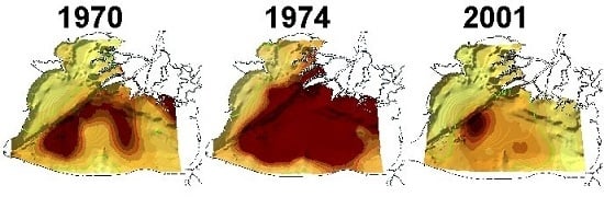
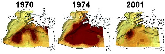
| Study Year | Minimum (µg/g) | Maximum (µg/g) | Average (µg/g) |
|---|---|---|---|
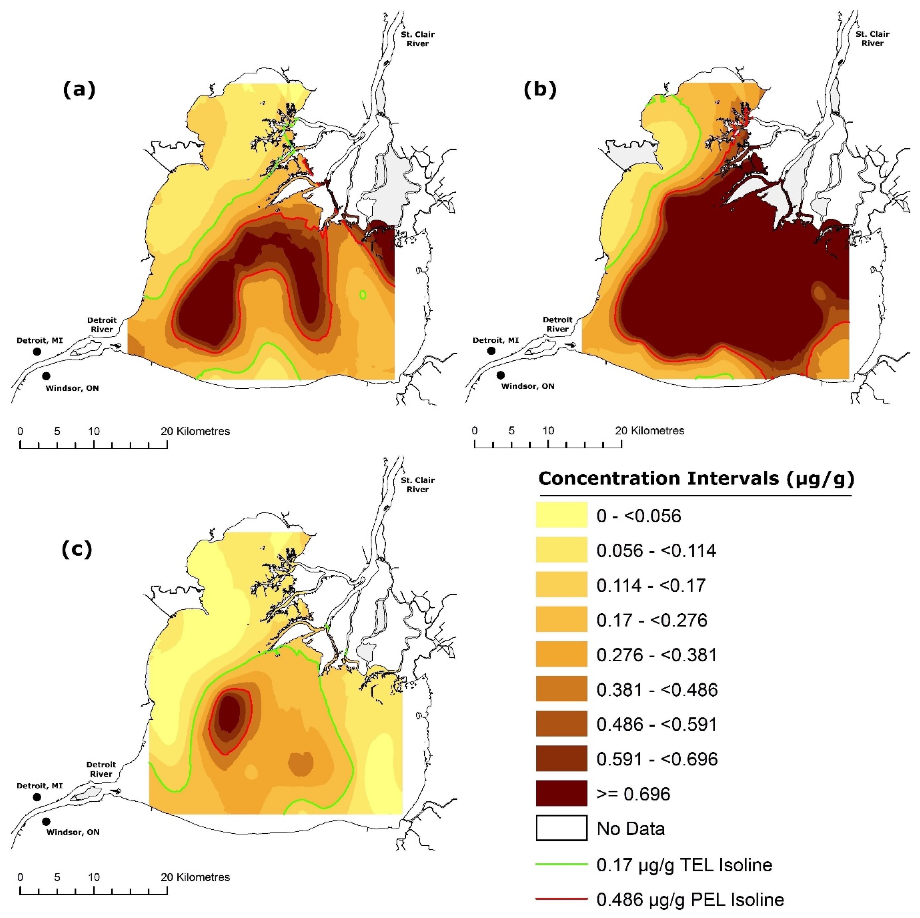
| 1970 | 0.030 | 3.640 | 0.566 |
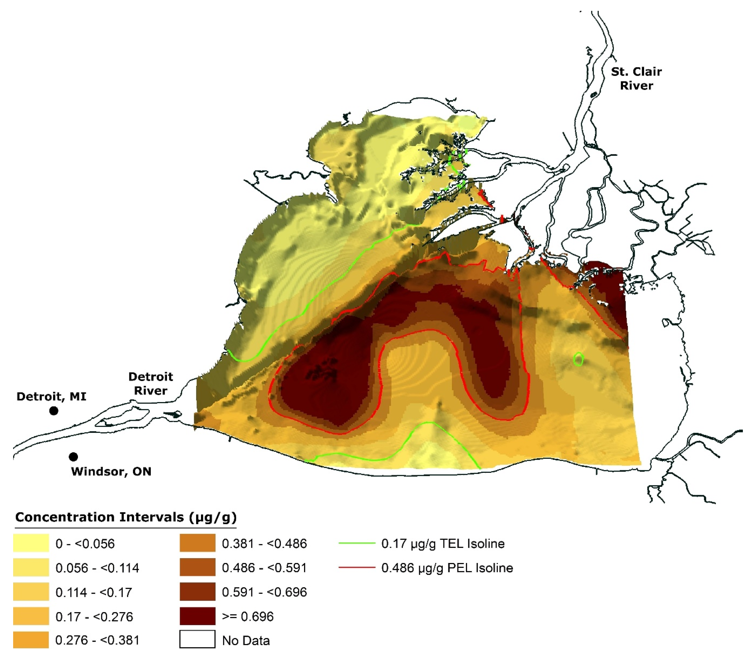
| 1974 | 0.050 | 10.280 | 1.585 |
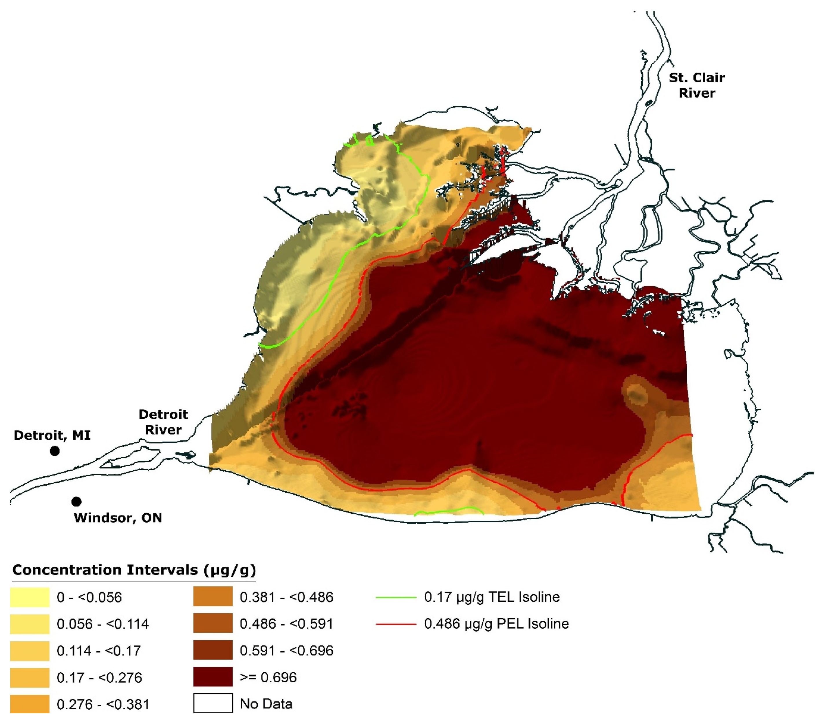
| 2001 | 0.005 | 1.194 | 0.190 |
| Study Year | MPE | ASE | SRMSPE |
|---|---|---|---|
| 1970 | 0.017 | 0.509 | 1.027 |
| 1974 | 0.026 | 0.543 | 0.931 |
| 2001 | 0.003 | 0.400 | 0.950 |
| Ideal | ~0.000 | <20.000 | ~1.000 |
© 2016 by the authors; licensee MDPI, Basel, Switzerland. This article is an open access article distributed under the terms and conditions of the Creative Commons Attribution license ( http://creativecommons.org/licenses/by/4.0/).
Share and Cite
Forsythe, K.W.; Marvin, C.H.; Valancius, C.J.; Watt, J.P.; Aversa, J.M.; Swales, S.J.; Jakubek, D.J.; Shaker, R.R. Geovisualization of Mercury Contamination in Lake St. Clair Sediments. J. Mar. Sci. Eng. 2016, 4, 19. https://doi.org/10.3390/jmse4010019
Forsythe KW, Marvin CH, Valancius CJ, Watt JP, Aversa JM, Swales SJ, Jakubek DJ, Shaker RR. Geovisualization of Mercury Contamination in Lake St. Clair Sediments. Journal of Marine Science and Engineering. 2016; 4(1):19. https://doi.org/10.3390/jmse4010019
Chicago/Turabian StyleForsythe, K. Wayne, Chris H. Marvin, Christine J. Valancius, James P. Watt, Joseph M. Aversa, Stephen J. Swales, Daniel J. Jakubek, and Richard R. Shaker. 2016. "Geovisualization of Mercury Contamination in Lake St. Clair Sediments" Journal of Marine Science and Engineering 4, no. 1: 19. https://doi.org/10.3390/jmse4010019
APA StyleForsythe, K. W., Marvin, C. H., Valancius, C. J., Watt, J. P., Aversa, J. M., Swales, S. J., Jakubek, D. J., & Shaker, R. R. (2016). Geovisualization of Mercury Contamination in Lake St. Clair Sediments. Journal of Marine Science and Engineering, 4(1), 19. https://doi.org/10.3390/jmse4010019