
An Oil Fate Model for Shallow-Waters


Abstract
:1. Introduction

2. Background
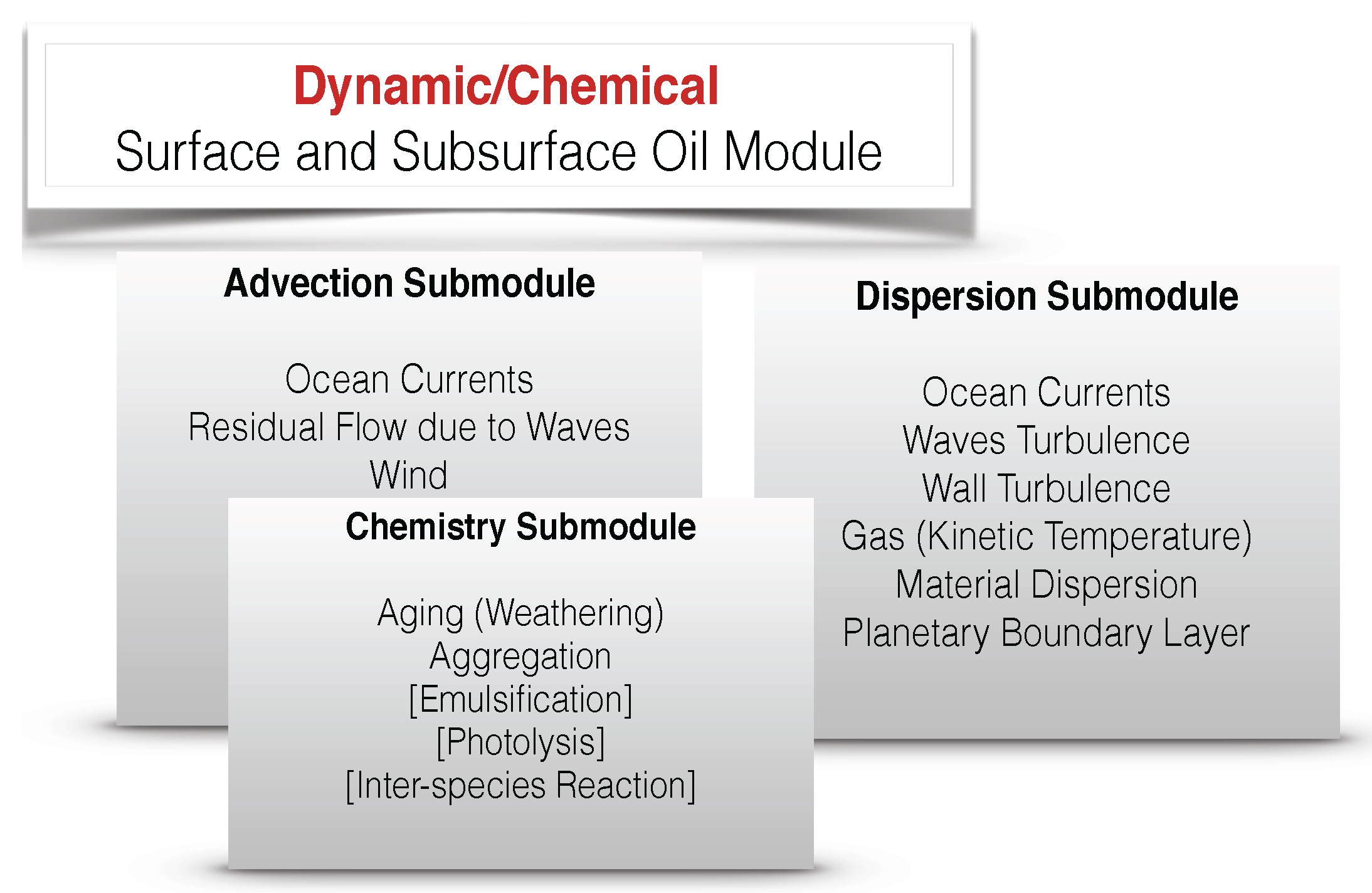
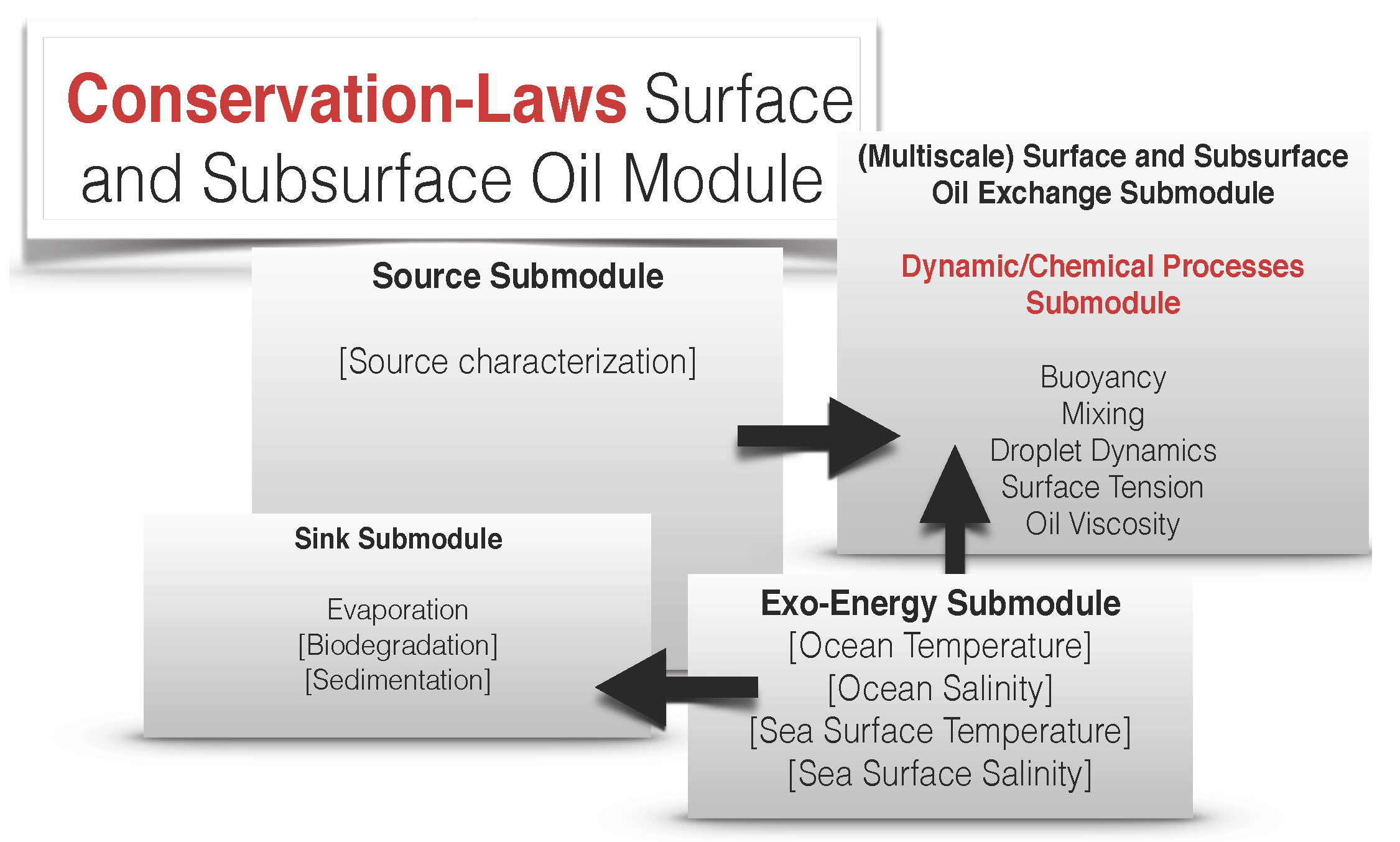
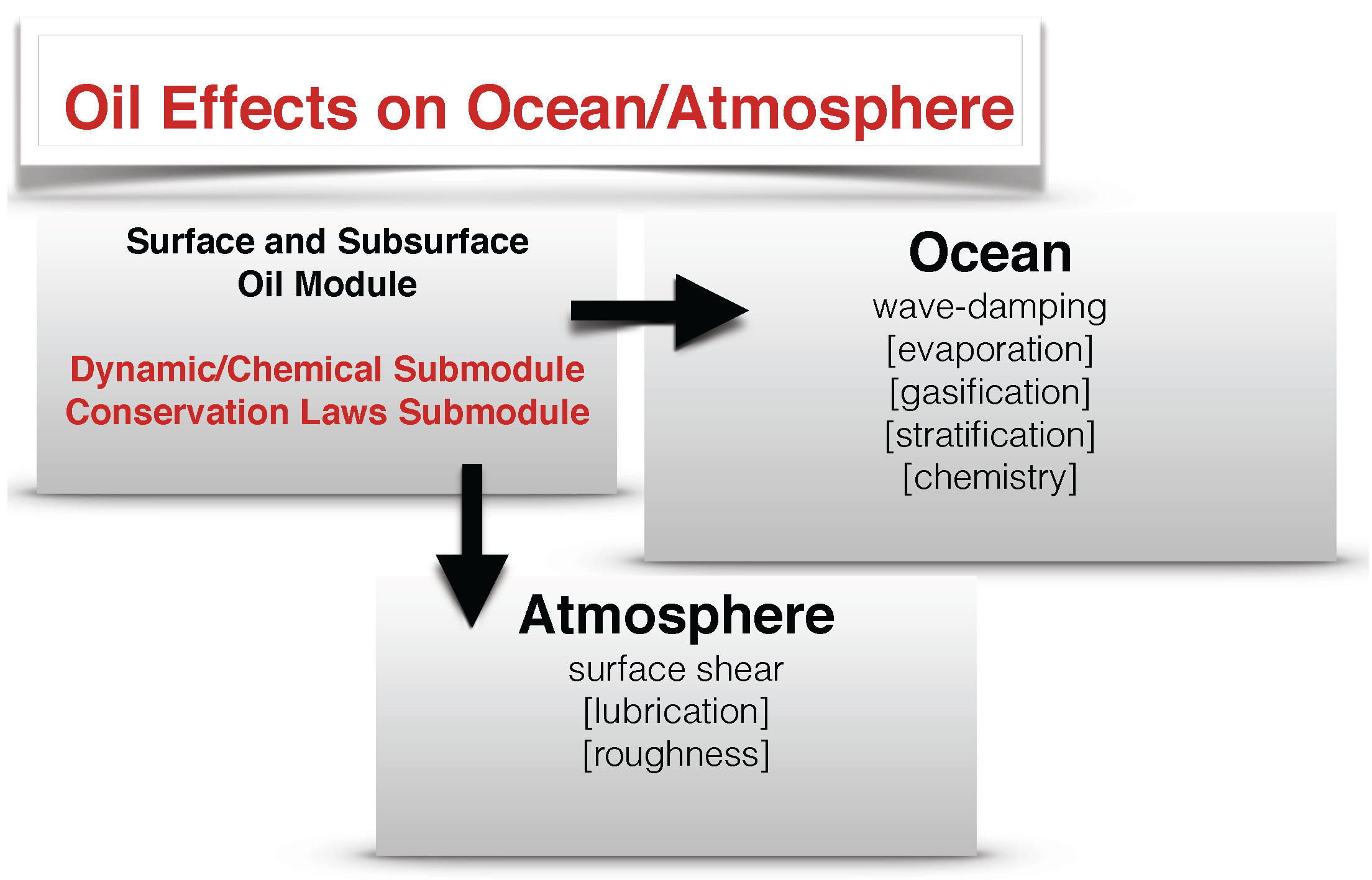
3. Oil Dynamics
3.1. The Oil Slick Component
3.2. The Sub-Surface Oil Component
3.3. Dispersion
3.4. Transformation Mechanisms: Chemistry and Physics of Oil
3.4.1. Mass Exchanges between the Subsurface Oil and the Slick
3.4.2. Aging: A Consequence of Grouping Chemicals and Unresolved Physics
3.4.3. Emulsification and Changes to the Density, Surface Tension, and Viscosity of the Slick
3.4.4. Evaporation
3.4.5. Photolysis, Biodegradation, Sedimentation
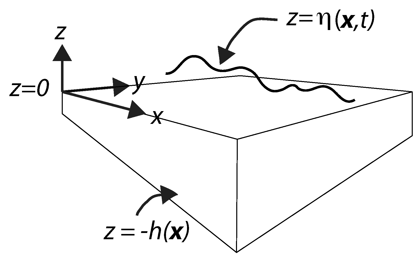
4. Ocean Dynamics
5. Energy Conservation
6. Illustrative Dynamic Examples
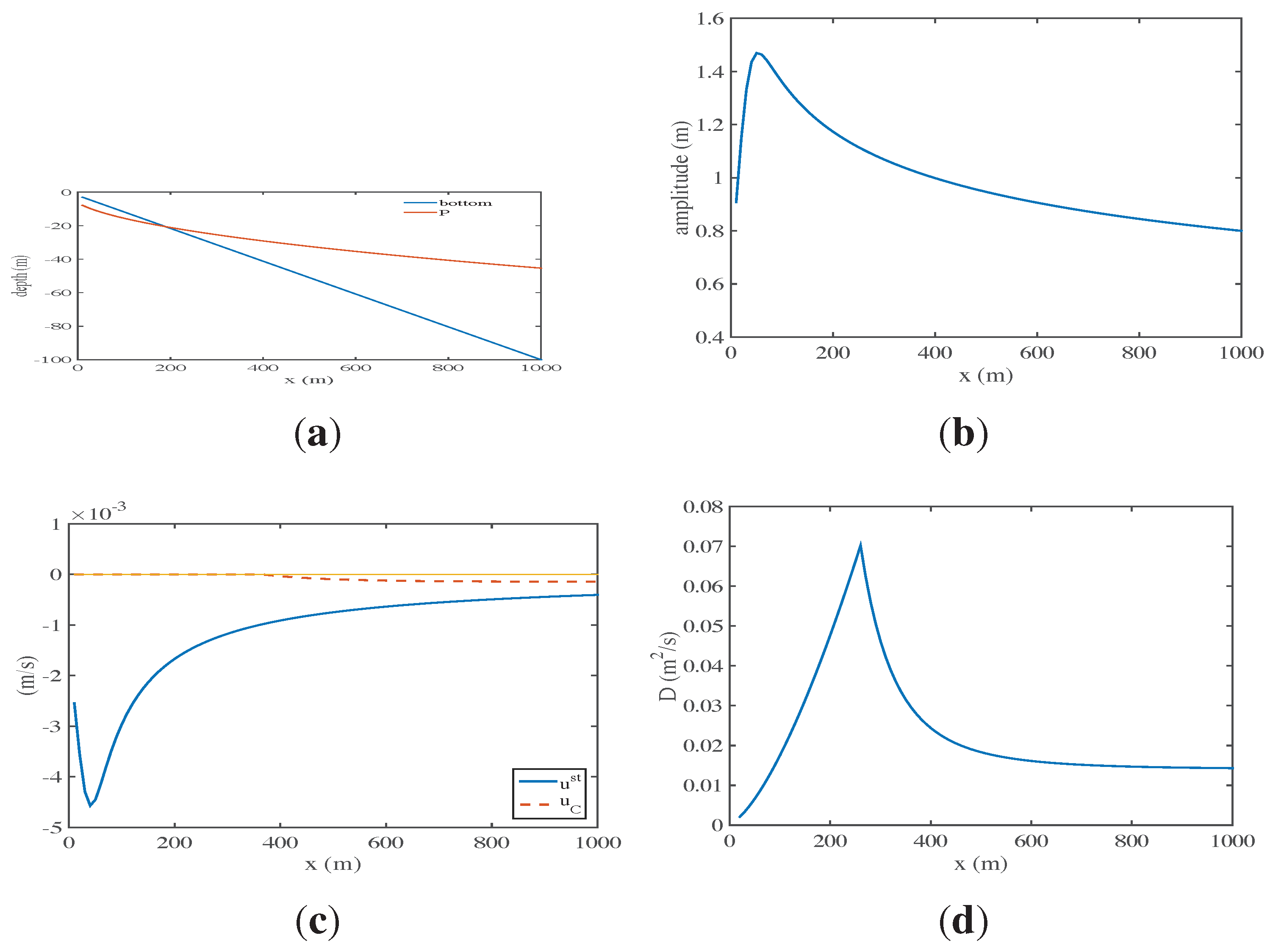
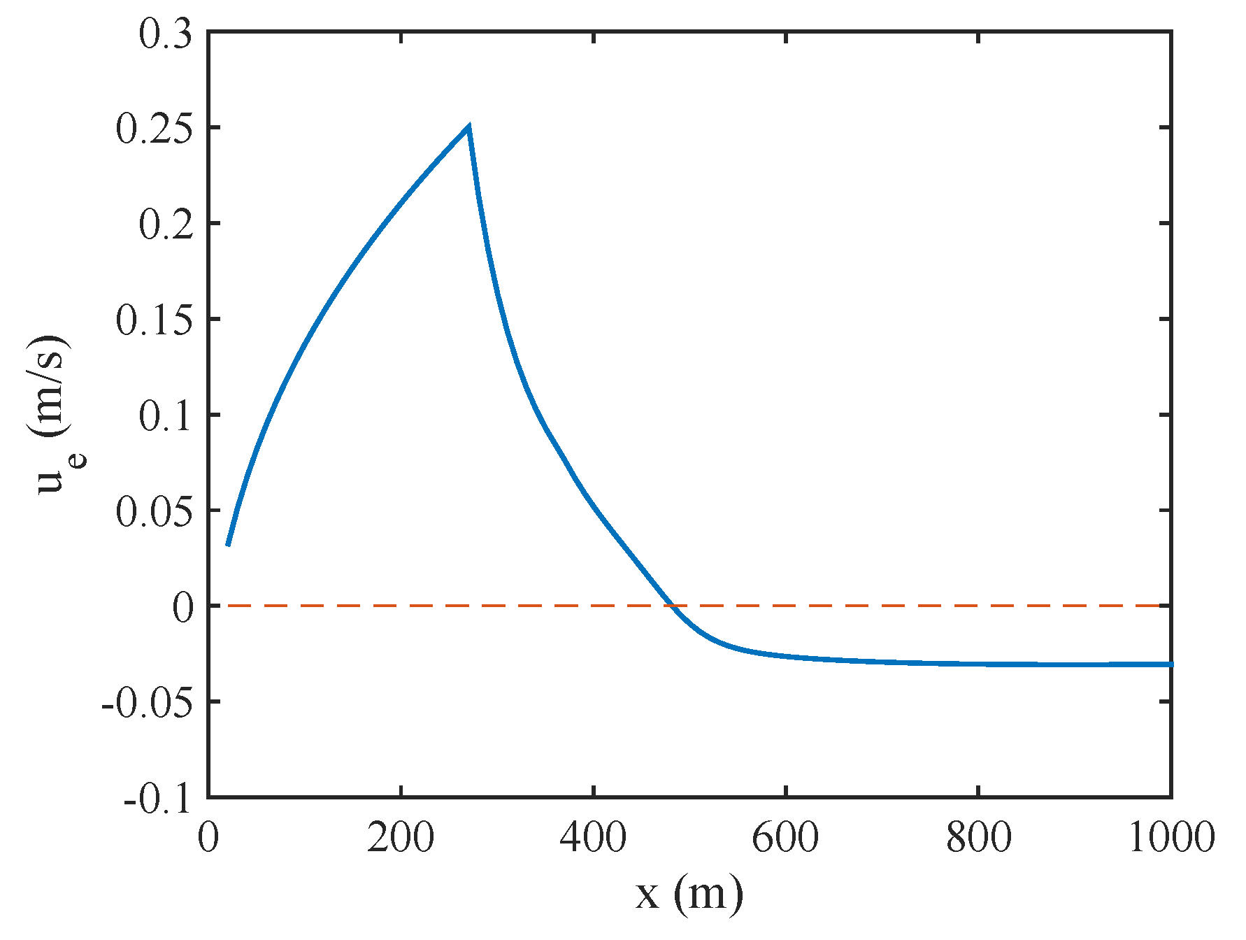
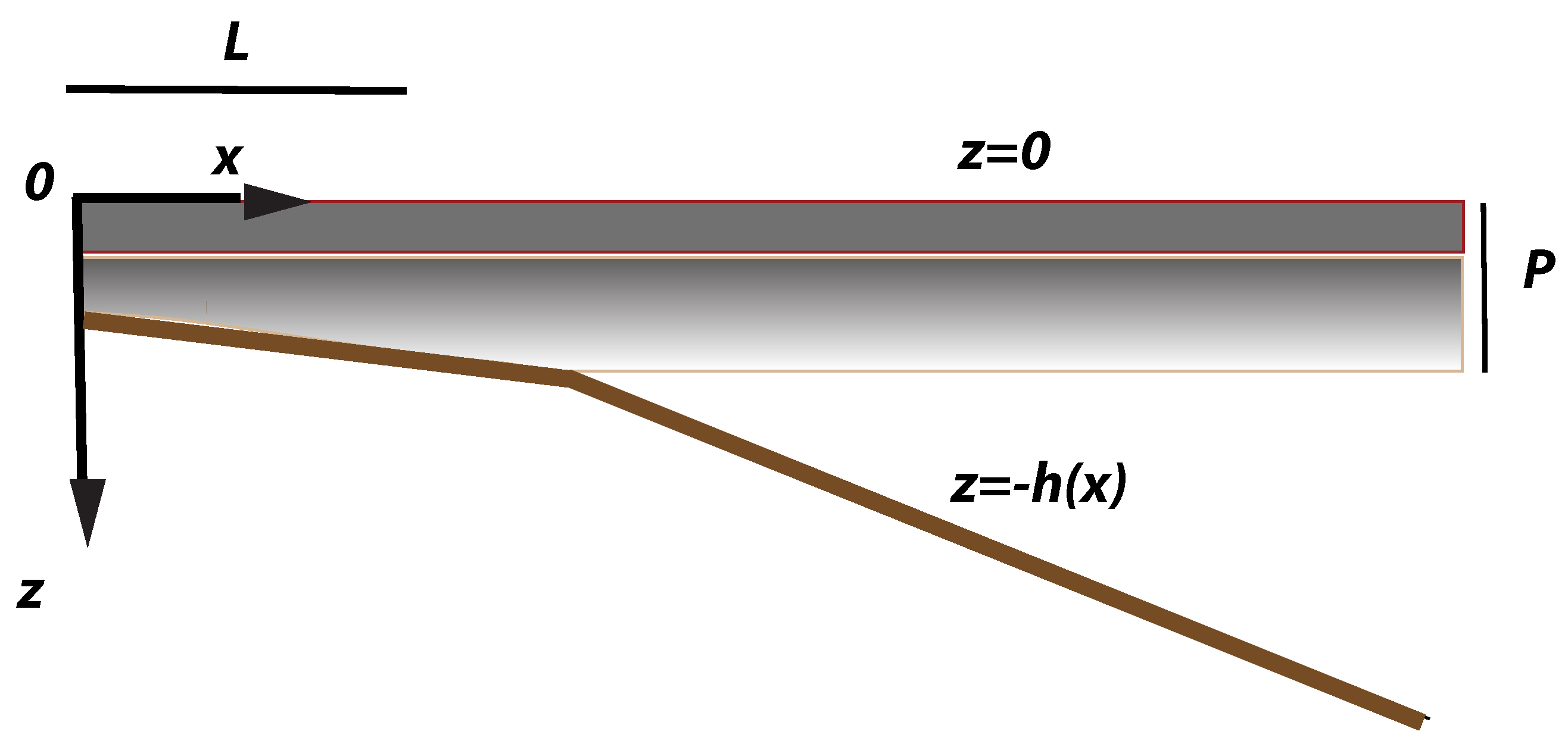
6.1. Nearshore Sticky Waters in Shores with Intense Breaking
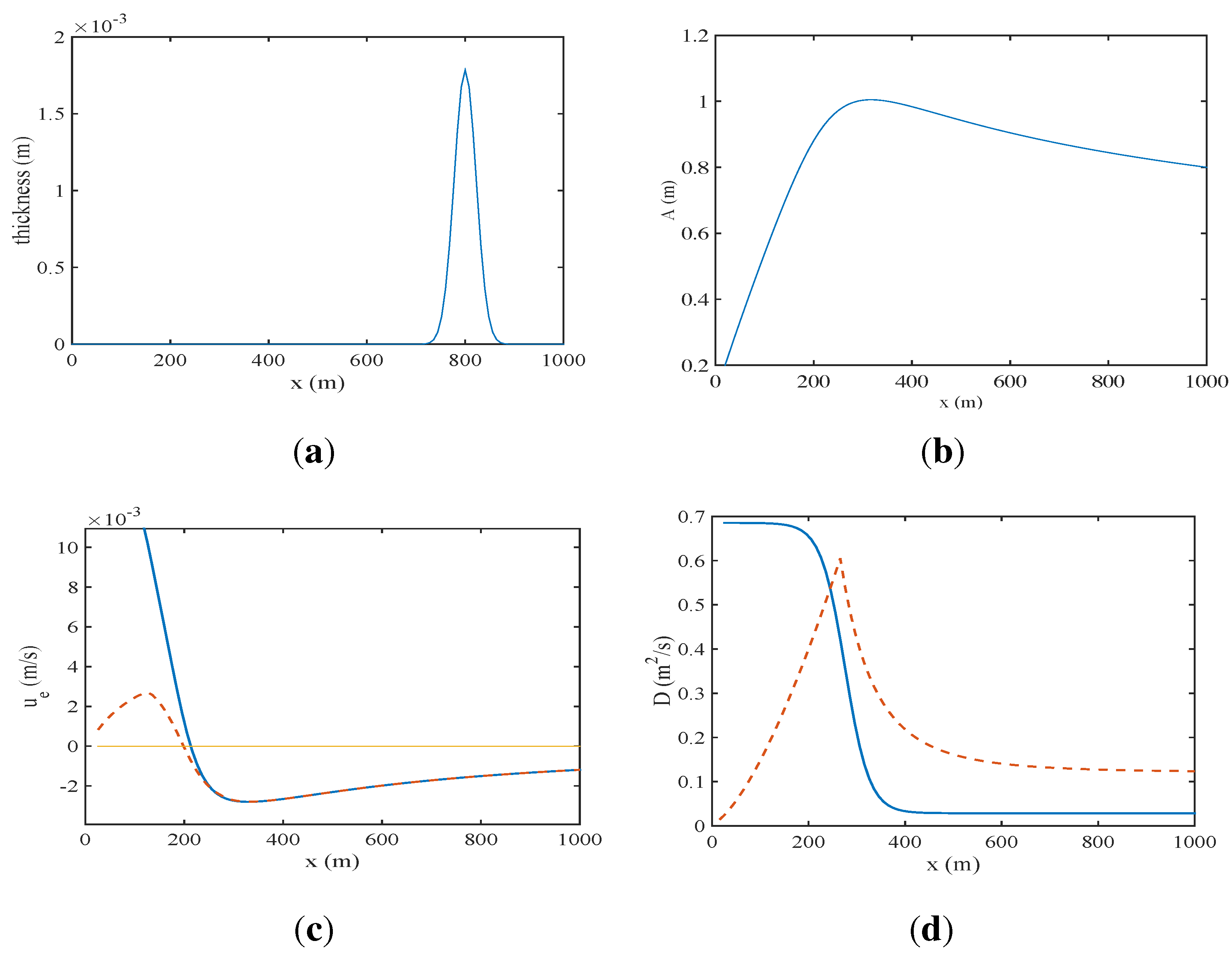
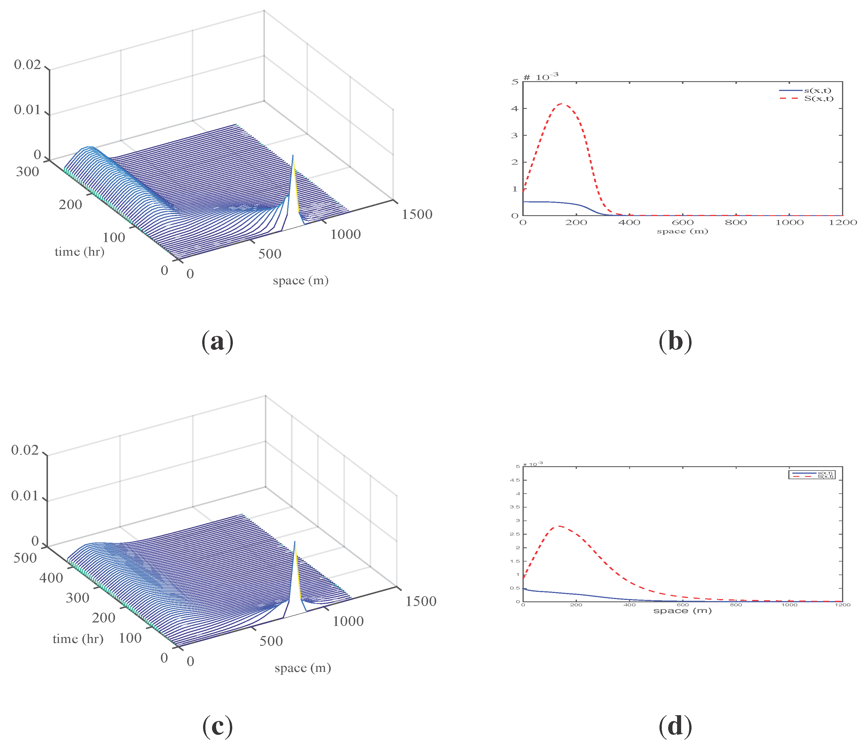


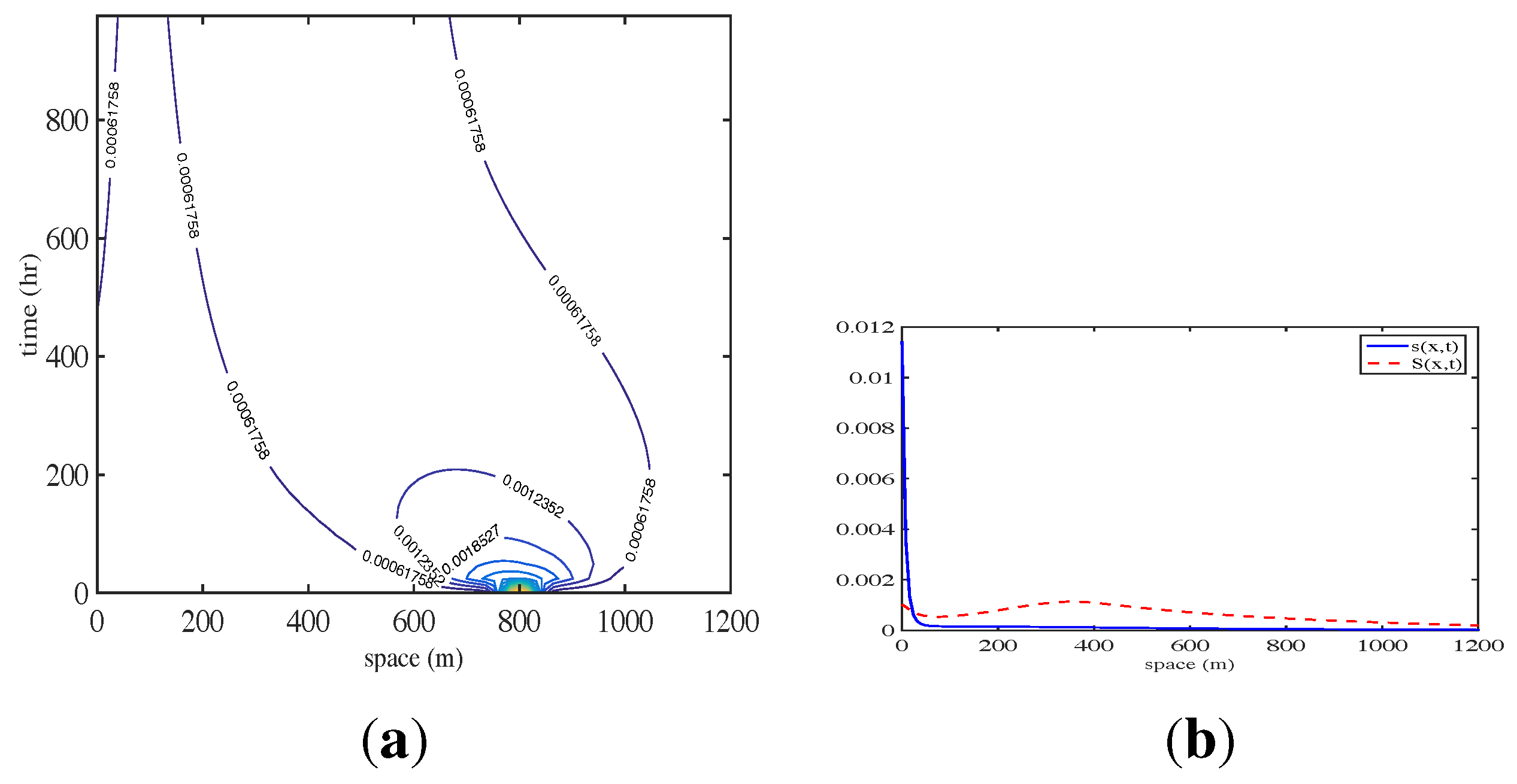
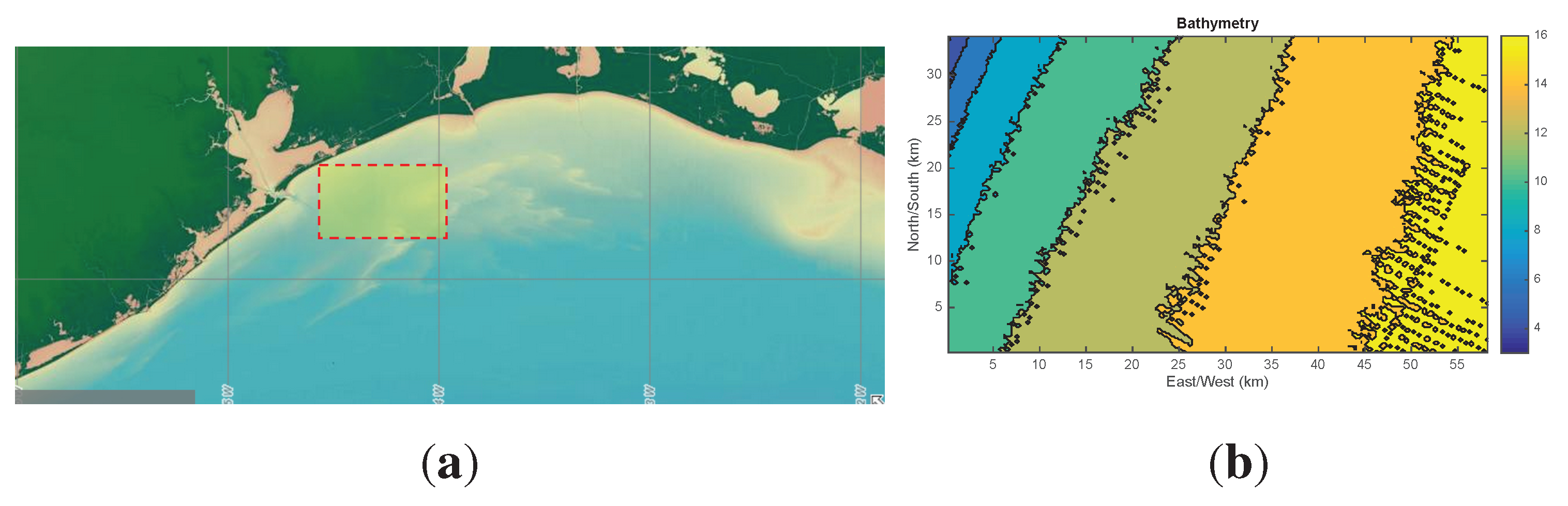
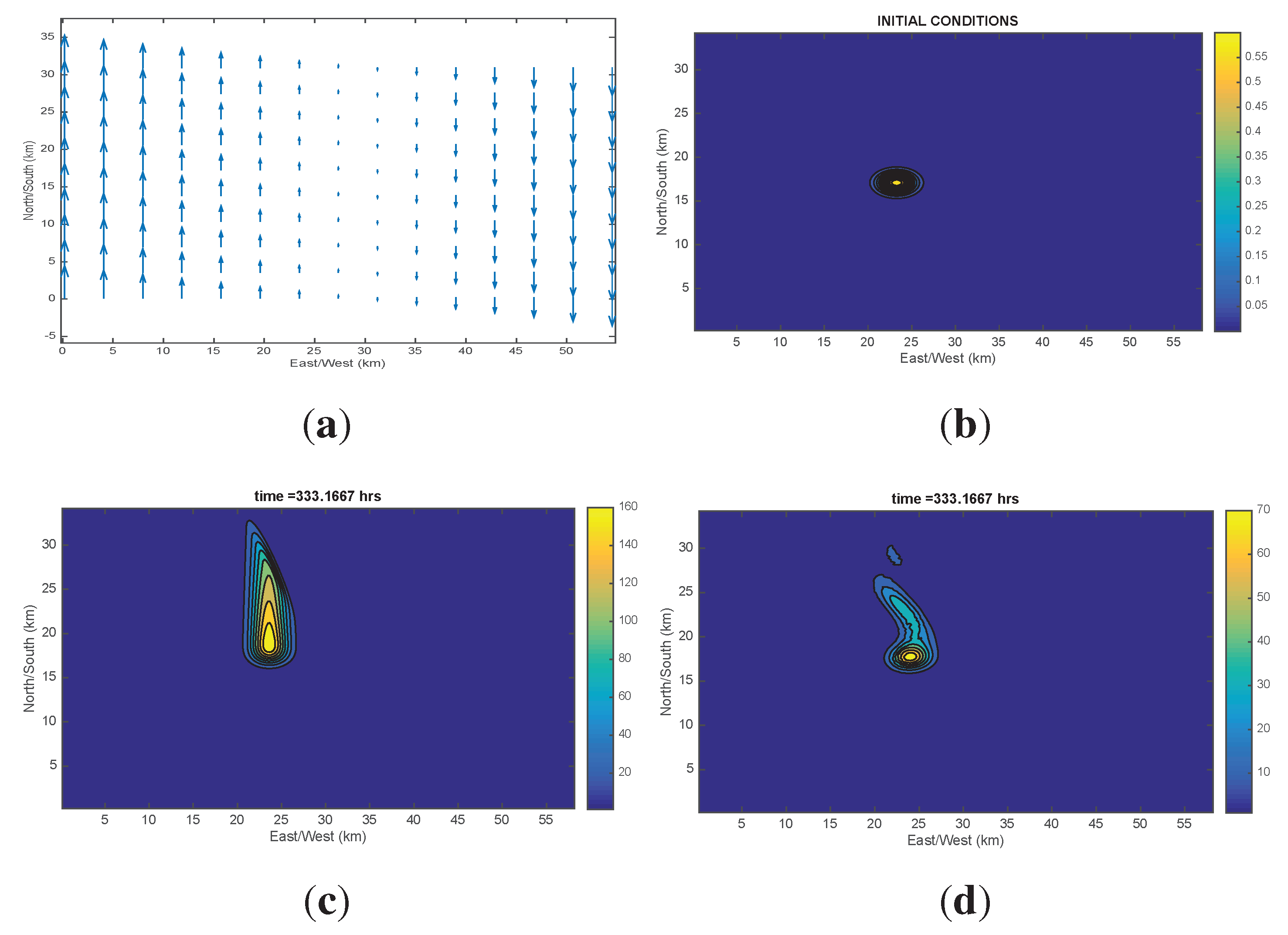
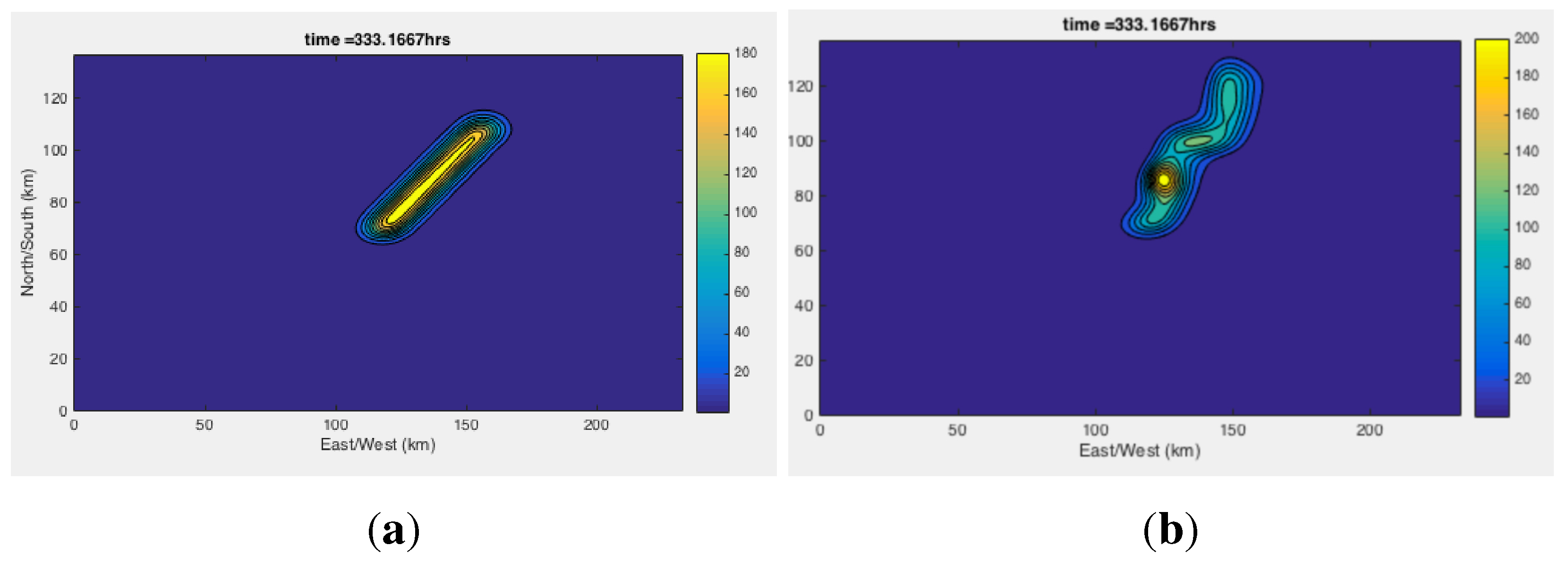
6.2. Shelf Dynamics Examples


7. Recapitulation
Acknowledgments
Author Contributions
Conflicts of Interest
Abbreviations
| Name | Symbol | Units |
| fast/slow time | t, T | s |
| transverse position vector. Cross-shore, along-shore coordinate | m | |
| depth coordinate | z | m |
| cross-shore, along-shore unit vectors | , | - |
| sea elevation | m | |
| bottom topography, total water column | h, | m |
| spatial gradient operator | 1/m | |
| wave and mean (current) sea elevation | , | m |
| density of water | Kg/m3 | |
| oil slick total mass | Kg | |
| thickness of i-th component of oil slick | m | |
| density of i-th oil slick component | Kg/m3 | |
| viscosity of i-th oil slick component | Kg/ms | |
| surface tension of i-th oil slick component | Kg/ms2 | |
| velocity of i-th oil slick component | 1/m2 | |
| depth averaged velocity of i-th oil slick component | m/s | |
| outward normal vector to ocean surface | - | |
| transverse component of wind stress | τ | Kg/ms2 |
| Eulerian ocean velocity at surface | m/s | |
| slip velocity parameter | - | |
| pressure, ambient plus dynamic | Kg/ms2 | |
| wave frequency, peak wave frequency | σ, | rad/s |
| depth-averaged transport velocity | m/s | |
| depth-averaged Eulerian velocity | m/s | |
| depth-averaged Stokes drift velocity | m/s | |
| tracer dispersion tensor | m2/s | |
| turbulent Reynolds stress tensor | Σ | m2/s |
| dispersion caused by averaging | Ξ | m2/s |
| dispersion due to fluctuations respect to friction velocity | Θ | m2/s |
| dispersion due to fluctuations respect to Stokes drift | m2/s | |
| friction velocity | m/s | |
| wind speed | m/s | |
| fractional water content | - | |
| fraction of evaporated oil from slick | - | |
| reaction, mass exchange, and other rates of oil slick | m/s | |
| total mass of subsurface oil | Kg | |
| concentration of i-th species | Kg/m3 | |
| generic tracer concentration | Kg/m3 | |
| ocean velocity | m/s | |
| tracer molecular diffusion | κ | m2/s |
| eddy flux tensor | Kg/s m2 | |
| parcel coordinate | m | |
| Kronecker delta tensor | δ | - |
| subsurface concentration associated with intermediate time scales | b | m3/m3 |
| wave covariance | m2 | |
| mixing layer thickness, oil mixed layer depth | P, | m |
| wave oil diffusion coefficient | m2/s | |
| indicator function of oil slick | - | |
| absolute and relative group velocity | , | m/s |
| unidirectional wave spectrum | F | s |
| Current forces: wind, breaking, bottom drag, lateral viscosity | , , , | |
| vortex force | ||
| vorticity, Coriolis constant | ω, | 1/s |
| wind drag parameter | - | |
| Manning drag parameter | - | |
| loss term in the action equation | ϵ | Kg/s |
| energy density | ||
| seafloor slope | m | m/m |
| surf zone extent | L | m |
| eddy viscosity | K | s |
| subsurface velocity | m/s | |
| subsurface effective bulk oil velocity | m/s | |
| effective thickness of submersed oil | S | m |
| nearshore bottom drag parameter | - |
References
- Maltrud, M.; Peacock, S.; Visbeck, M. On the possible long-term fate of oil released in the Deepwater Horizon incident, estimated using ensembles of dye release simulations. Environ. Res. Lett. 2010, 5, 035301. [Google Scholar] [CrossRef]
- Liu, Y.; Macfadyen, A.; Ji, Z.G.; Weisberg, R.H.; Huntley, H.S.; Lipphardt, B.L.; Kirwan, A.D. Surface drift predictions of the Deepwater Horizon spill: The Lagrangian perspective. Environ. Sci. Technol. 2013, 46, 7267–7273. [Google Scholar]
- Mariano, A.; Kourafaloua, V.; Srinivasana, A.; Kanga, H.; Halliwell, G.; Ryana, E.; Roffer, M. On the modeling of the 2010 Gulf of Mexico oil spill. Dyn. Oceans Atmos. 2011, 52, 311–322. [Google Scholar] [CrossRef]
- Wang, J.; Shen, Y. Modeling oil spills transportation in seas based on unstructured grid, finite-volume, wave-ocean model. Ocean Model. 2012, 35, 332–344. [Google Scholar] [CrossRef]
- Tkalich, P.; Chan, E.S. A CFD solution of oil spill problems. Environ. Model. Softw. 2006, 21, 271–282. [Google Scholar] [CrossRef]
- Papadimitrakis, J.; Psaltaki, M.; Christolis, M.; Markatos, N.C. Simulating the fate of an oil spill near coastal zones: The case of a spill (from a power plant) at the Greek island of Lesvos. Environ. Model. Softw. 2006, 21, 170–177. [Google Scholar] [CrossRef]
- Azevedo, A.; Oliveira, A.; Fortunato, A.B.; Zhang, J.; Baptista, A.M. A cross-scale numerical modeling system for management support of oil spill accidents. Mar. Pollut. Bull. 2014, 80, 132–147. [Google Scholar] [CrossRef] [PubMed]
- Seymour, R.J.; Geyer, R. Fates and Effects of Oil Spills. Annu. Rev. Energy Environ. 1992, 17, 261–283. [Google Scholar] [CrossRef]
- Feddersen, F. Observations of the surf-zone turbulent dissipation rate. J. Phys. Oceanogr. 2012, 42, 386–399. [Google Scholar] [CrossRef]
- Feddersen, F. Scaling surf zone turbulence. Geophys. Res. Lett. 2012, 39. [Google Scholar] [CrossRef]
- Fingas, M.F.; Duval, W.; Stevenson, G.B. The Basics of Oil Spill Cleanup; Minister of Supply and Services: Quebec, Canada, 1979. [Google Scholar]
- Payne, J.R.; Philips, C. Petroleum Spills in the Marine Environment: Chemistry and Formation of Water-in-Oil Emulsions and Tar Balls; Lewis Publishers: Chelsea, MI, USA, 1985. [Google Scholar]
- Zhang, X.; Hetland, R.; Marta-Almeida, M.; DiMarco, S.F. A numerical investigation of the Mississippi and Atchafalaya freshwater transport, filling and flushing times on the Texas-Louisiana Shelf. J. Geophys. Res. Oceans 2012, 117, 5705–5723. [Google Scholar] [CrossRef]
- Zhang, Z.; Hetland, R.; Zhang, X. Wind-modulated buoyancy circulation over the Texas-Lousiana Shelf. J. Geophys. Res. Oceans 2013, 119, 5705–5723. [Google Scholar] [CrossRef]
- Warner, J.D.; Geyer, W.R.; Lerczak, J.A. Numerical modeling of an estuary: A comprehensive skill assessment. J. Geophys. Res. Oceans 2005, 110. [Google Scholar] [CrossRef]
- Hetland, R.D. Event driven model skill assessment. Ocean Model. 2006, 11, 214–223. [Google Scholar] [CrossRef]
- Howlett, E.; Jayko, K. COZOIL (Coastal Zone Oil Spill Model), Improvements and Linkage to a Graphical User Interface. In Proceedings of the Twenty-First Artic and Marine Oilspill Program (AMOP) Technical Seminar, Alberta, Canada, 10–12 June 1998; Volume 21, pp. 541–550.
- Zhao, L.; Torlapati, J.; Boufadel, M.; King, T.; Robinson, B.; Lee, K. VDROP: A Comprehensive model for droplet formation of oils and gases in liquids—Incorporation of the interfacial tension and droplet viscosity. Chem. Eng. J. 2014, 253, 93–106. [Google Scholar] [CrossRef]
- McWilliams, J.C.; Restrepo, J.M.; Lane, E.M. An asymptotic theory for the interaction of waves and currents in coastal waters. J. Fluid Mech. 2004, 511, 135–178. [Google Scholar] [CrossRef]
- Lehr, W.J. Review of modeling procedures for oil spill weathering behavior. In Advances in Ecological Models; Brebbia, C.A., Ed.; WIT Press: Southampton, UK, 2001; Chapter 3. [Google Scholar]
- McWilliams, J.C.; Restrepo, J.M. The wave-driven ocean circulation. J. Phys. Oceanogr. 1999, 29, 2523–2540. [Google Scholar] [CrossRef]
- Restrepo, J.M.; Ramírez, J.M.; McWilliams, J.C.; Banner, M. Multiscale momentum flux and diffusion due to whitecapping in wave–current interactions. J. Phys. Oceanogr. 2011, 41, 837–856. [Google Scholar] [CrossRef]
- Garrett, C. Turbulent dispersion in the ocean. Progress Oceanogr. 2006, 70, 113–125. [Google Scholar] [CrossRef]
- Kim, D.H.; Lynett, P.J. Turbulent mixing and passive scalar transport in shallow flows. Phys. Fluids 2011, 23, 016603. [Google Scholar] [CrossRef]
- Atlas, R.M.; Hazen, T.C. Oil biodegradation and bioremediation: A tale of the two torst spills in U.S. history. Environ. Sci. Technol. 2011, 45, 6709–6715. [Google Scholar] [CrossRef] [PubMed]
- Moghimi, S.; Restrepo, J.M.; Venkataramani, S. Mass conservation modeling in an oil fate model for shallow waters. J. Mar. Sci. Eng. 2016. submitted for publication. [Google Scholar]
- Lasheras, J.C.; Eastwood, C.; Martínez-Bazán, C.; Montanés, J. A review of statistical models for the break-up of an immiscible fluid immersed into a fully turbulent flow. Int. J. Multiph. Flows 2002, 28, 247–278. [Google Scholar] [CrossRef]
- Boehm, P.; Flest, D.L.; Mackay, D.; Paterson, S. Physical-chemical weathering of petroleum hydrocarbons from the Ixtoc I blowout: Chemical measurements and a weathering model. Environ. Sci. Technol. 1982, 16, 498–504. [Google Scholar] [CrossRef]
- Cuesta, I.; Grau, F.X.; Giralt, F. Numerical simulation of oil spills in a generalized domain. Oil Chem. Pollut. 1990, 7, 143–159. [Google Scholar] [CrossRef]
- Quinn, M.F.; Marron, K.; Paten, B.; Abu-Tabanja, R.; Al-Bahrani, H. Modeling of the ageing of crude oils. Oil Chem. Pollut. 1990, 7, 119–128. [Google Scholar] [CrossRef]
- Buchanan, I.; Hurford, N. Methods for predicting physical changes in oil spilt at sea. Oil Chem. Pollut. 1988, 4, 311–328. [Google Scholar] [CrossRef]
- Sebastiao, P.; Soares, C.G. Modeling the fate of oil spills at sea. Spill Sci. Technol. Bull. 1995, 2, 121–131. [Google Scholar] [CrossRef]
- Reed, M.; Gundlach, E.; Kana, T. A coastal zone poil spill model: Development and sensitivity studies. Oil Chem. Pollut. 1989, 5, 411–449. [Google Scholar] [CrossRef]
- Mooney, M. The viscosity of a concentrated suspection of spherical particles. J. Colloidal Sci. 1951, 10, 162–170. [Google Scholar] [CrossRef]
- Mackay, D.; Shiu, W.Y.; Hossain, K.; Stiver, W.; McCurdy, D.; Paterson, S.; Tebeau, P. Development and Calibration of an Oil Spill Behaviour Model; CG-D-27-83; US Coast Guard Research and Development Center: Washington, DC, USA, 1982. [Google Scholar]
- Xie, H.; Yappa, P.D.; Nakata, K. Modeling emulsification after an oil spill in the sea. J. Mar. Syst. 2007, 68, 489–506. [Google Scholar] [CrossRef]
- Stiver, W.; Mackay, D. Evaporation rate of spills of hydrocarbons and petroleum mixtures. Environ. Sci. Technol. 1984, 18, 834–840. [Google Scholar] [CrossRef] [PubMed]
- Stiver, W.; Shiu, W.Y.; Mackay, D. Evaporation times and rates of specific hydrocarbons in oil spills. Environ. Sci. Technol. 1989, 23, 101–105. [Google Scholar] [CrossRef]
- Mackay, D.; Matsugu, R.S. Evaporation Rates of liquid hydrocarbon spills on land and water. Can. J. Chem. Eng. 1973, 51, 434–439. [Google Scholar] [CrossRef]
- Bobra, M. A Study of the Evaporation of Petroleum Oils; MR EE-135; Environment Canada, Environmental Protection Directorate: River Road Environmental Technology Centre, 1992. [Google Scholar]
- Smith, C.L.; McIntyre, W.G. Initial Ageing of Fuel Oils on Sea Water. In Proceedings of the Joint Conference on Prevention and Control of Oil Spills, Washington, DC, USA, 15–17 June 1971; pp. 457–461.
- Fingas, M. A literature review of the physics and predictive modeling of oil spill evaporation. J. Hazard. Mater. 1995, 42, 157–175. [Google Scholar] [CrossRef]
- Payne, J.R.; Phillips, C.W. Photochemistry of oil in water. Environ. Sci. Technol. 1985, 19, 569–579. [Google Scholar] [CrossRef] [PubMed]
- Spaulding, M.L. A state-of-the-art review of oil spill trajectory and fate modeling. Oil Chem. Pollut. 1988, 4, 39–55. [Google Scholar] [CrossRef]
- Webb, A.; Fox-Kemper, B. Wave spectral moments and Stokes drift estimation. Ocean Model. 2011, 40, 273–288. [Google Scholar] [CrossRef]
- Church, J.C.; Thornton, E.B. Effects of breaking wave induced turbulence within a longshore current model. Coast. Eng. 1993, 20, 1–28. [Google Scholar] [CrossRef]
- Thornton, E.B.; Guza, R.T. Transformation of wave height distribution. J. Geophys. Res. 1983, 88, (C10). 5925–5938. [Google Scholar] [CrossRef]
- Venkataramani, S.C.; Venkataramani, R.; Restrepo, J.M. Stochastic parametrization of weathering processes. Phys. Rev. E 2016. submitted for publication. [Google Scholar]
- Restrepo, J.M.; Venkataramani, S.C.; Dawson, C. Nearshore sticky waters. Ocean Model. 2014, 80, 49–58. [Google Scholar] [CrossRef]
- Restrepo, J.; Venkataramani, S.; Balci, N. Stochastic longshore dynamics equations. Ocean Model. 2015. under review. [Google Scholar]
- Longuet-Higgins, M.S. Longshore currents generated by obliquely incident sea waves: 1 & 2. J. Geophys. Res. 1970, 75, 6778–6801. [Google Scholar]
- Svendsen, I.A.; Putrevu, U. Surf-zone hydrodynamics. Adv. Coast. Ocean Eng. 1995, 2, 1–78. [Google Scholar]
- Thornton, E.B.; Guza, R.T. Surf zone longshore currents and random waves: Field data and models. J. Phys. Oceanogr. 1986, 16, 1165–1178. [Google Scholar] [CrossRef]
- Guannel, G.; Özkan-Haller, H.T. Formulation of the undertow using linear wave theory. Phys. Fluids 2014, 26, 056604. [Google Scholar] [CrossRef]
- McWilliams, J.C.; Sullivan, P.P.; Moeng, C.H. Langmuir turbulence in the ocean. J. Fluid Mech. 1997, 334, 1–30. [Google Scholar] [CrossRef]
- Johnson, D.R. Ocean Surface Current Climatology in the Northern Gulf of Mexico; Gulf Coast Research Laboratory: Ocean Springs, MS, USA, 2008. [Google Scholar]
- Bathymetric Data Viewer. Available online: http://maps.ngdc.noaa.gov/viewers/bathymetry/ (accessed on 2 December 2015).
- McWilliams, J.C. A perspective on submesoscale geophysical turbulence. In IUTAM Symposium on Turbulence in the Atmosphere and Oceans; Dritschel, D., Ed.; Springer: Berlin, Germany, 2010; pp. 131–141. [Google Scholar]
- Capet, X.; McWilliams, J.C.; Molemaker, M.J.; Shchepetkin, A. Mesoscale to submesoscale transition in the California Current System. Part I: Flow structure, eddy flux, and observational tests. J. Phys. Oceanogr. 2008, 38, 29–43. [Google Scholar] [CrossRef]
- Shchepetkin, A.F.; McWilliams, J. The regional oceanic modeling system (ROMS): A split-explicit, free-surface, topography-following-coordinate oceanic model. Ocean Model. 2005, 9, 347–404. [Google Scholar] [CrossRef]
© 2015 by the authors; licensee MDPI, Basel, Switzerland. This article is an open access article distributed under the terms and conditions of the Creative Commons Attribution license ( http://creativecommons.org/licenses/by/4.0/).
Share and Cite
Restrepo, J.M.; Ramírez, J.M.; Venkataramani, S. An Oil Fate Model for Shallow-Waters. J. Mar. Sci. Eng. 2015, 3, 1504-1543. https://doi.org/10.3390/jmse3041504
Restrepo JM, Ramírez JM, Venkataramani S. An Oil Fate Model for Shallow-Waters. Journal of Marine Science and Engineering. 2015; 3(4):1504-1543. https://doi.org/10.3390/jmse3041504
Chicago/Turabian StyleRestrepo, Juan M., Jorge M. Ramírez, and Shankar Venkataramani. 2015. "An Oil Fate Model for Shallow-Waters" Journal of Marine Science and Engineering 3, no. 4: 1504-1543. https://doi.org/10.3390/jmse3041504
APA StyleRestrepo, J. M., Ramírez, J. M., & Venkataramani, S. (2015). An Oil Fate Model for Shallow-Waters. Journal of Marine Science and Engineering, 3(4), 1504-1543. https://doi.org/10.3390/jmse3041504