1. Introduction
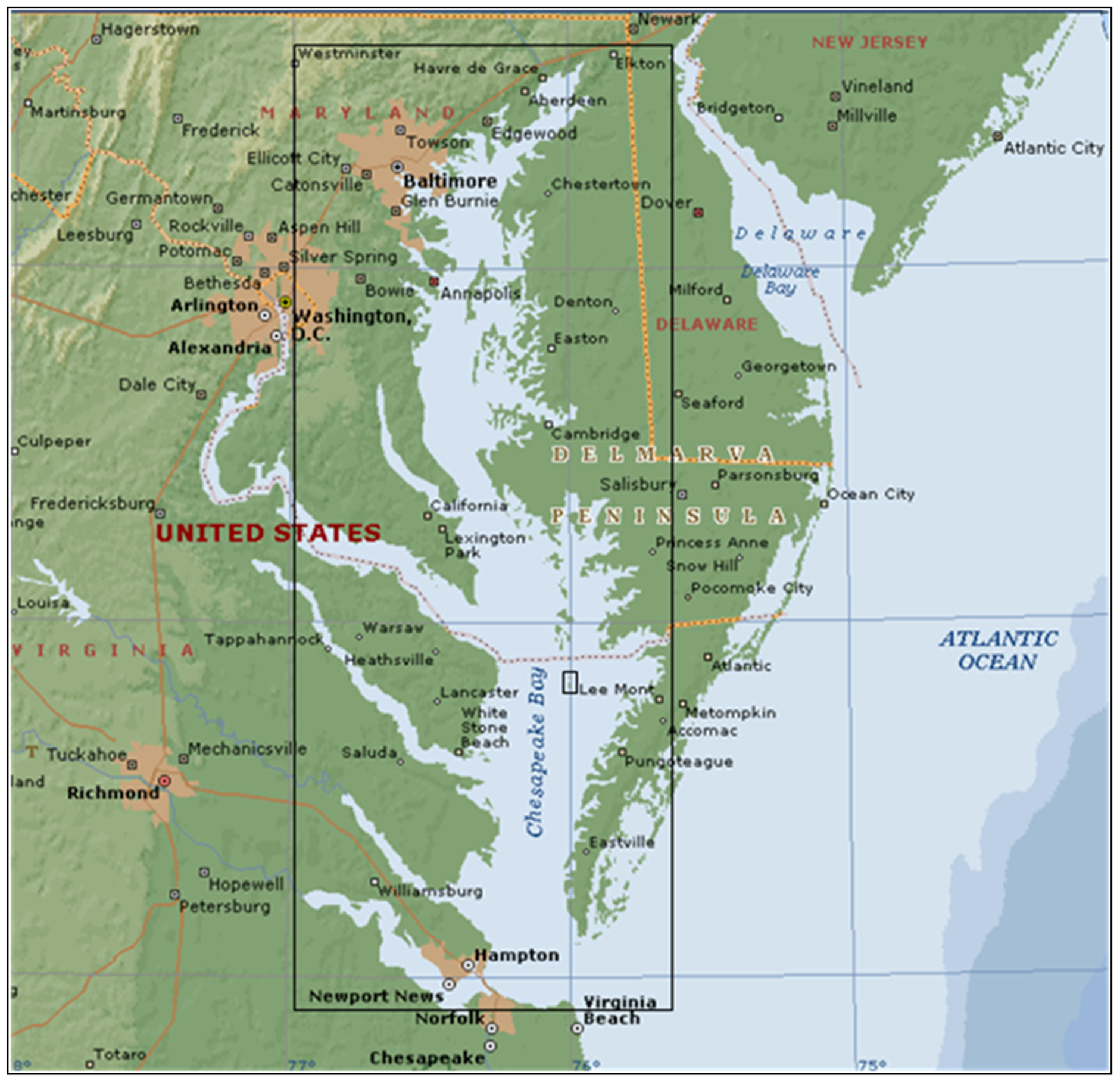
Tangier Island (75°59.4′ W, 37°49.8′ N) is the southernmost of a string of islands. The shallower Tangier Sound separates the lower Chesapeake Bay on the west from the east bay (
Figure 1). The island, approximately 8 km (5 miles) long by 3.2 km (2 miles) wide, is located in the Virginia portion of Chesapeake Bay, 36 km (20 miles) southwest of Crisfield and 112 km (70 miles) north of Norfolk. Tangier Island is comprised of a few low fine-grained sand ridges with intervening marshlands having numerous islets and tidal creeks. The highest elevations of the island are only a few meters above the mean tide level (MTL). The small populated areas are primarily three interconnected ridges on the south-central portion of the island.
Figure 1.
Location of Tangier Island (small rectangular box) in Chesapeake Bay (large box).
Figure 1.
Location of Tangier Island (small rectangular box) in Chesapeake Bay (large box).
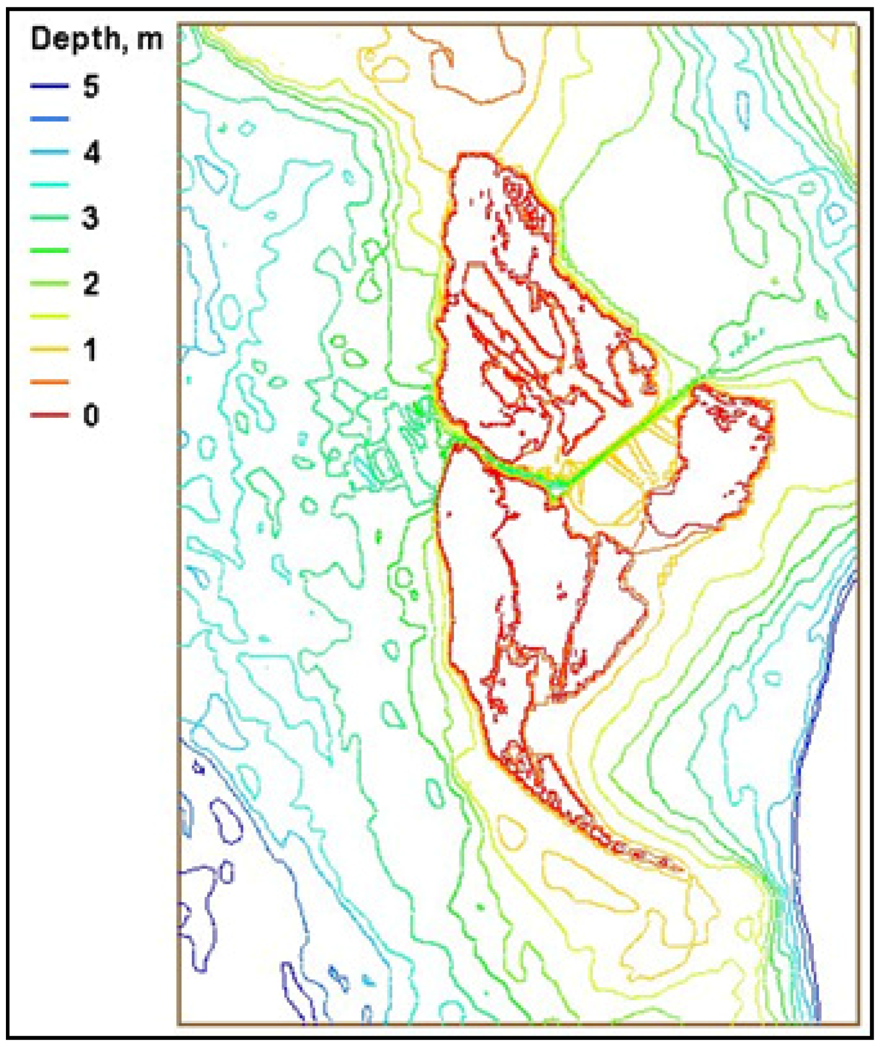
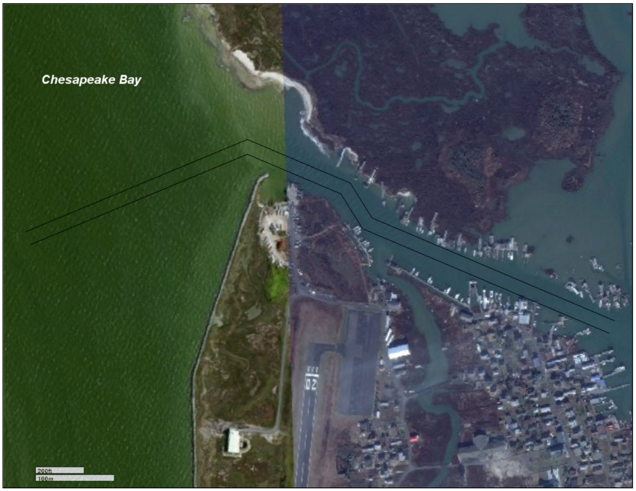
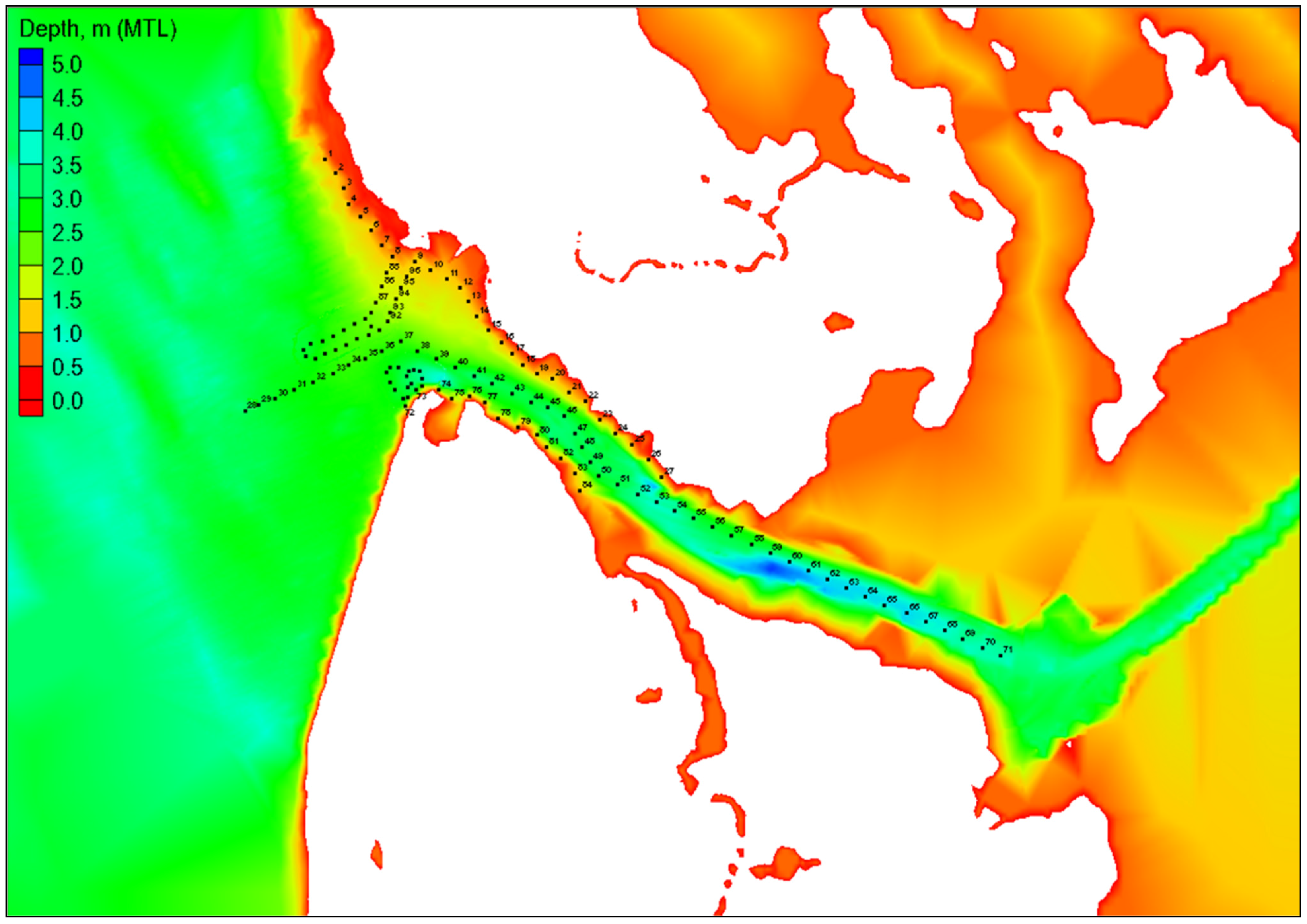
Tangier Island boat canal is a narrow light-draft channel that runs east–west across the mid-section of the island (
Figure 2). It is approximately 2.3 km (1.5 miles) long, 80 m (265 ft) wide, and 4 m (13 ft) deep for small-boat traffic. Numerous mooring docks and seafood processing sheds along both sides of the canal are the main infrastructure of local fishing and crabbing industries.
Figure 2.
Depth contours in the boat canal crossing through the mid-section of Tangier Island.
Figure 2.
Depth contours in the boat canal crossing through the mid-section of Tangier Island.
The western side of Tangier Island is exposed to large incident waves (up to 2-m wave height) generated during storms in the Chesapeake Bay from the northwest through southwest quadrants. The western shoreline has long experienced progressive flooding and erosion during storms. Due to prevailing wind patterns, the littoral transport along the west shorelines of the island is directed toward the south. During storms, large waves with strong currents and high water frequently enter the western entrance of the boat canal, causing damage to shorelines and structures.
The U.S. Army Corps of Engineers (USACE) Research and Development Center (ERDC) has conducted a numerical modeling study of waves and hydrodynamics for jetty alternatives intended to protect shorelines and reduce wave energy in the western portion of the canal. The primary goal of the study was to develop a quantitative estimate of waves and wave reduction in the canal for alternatives with minimal effects on channel dredging requirements and boat traffic in the channel.
2. Local Environmental Conditions
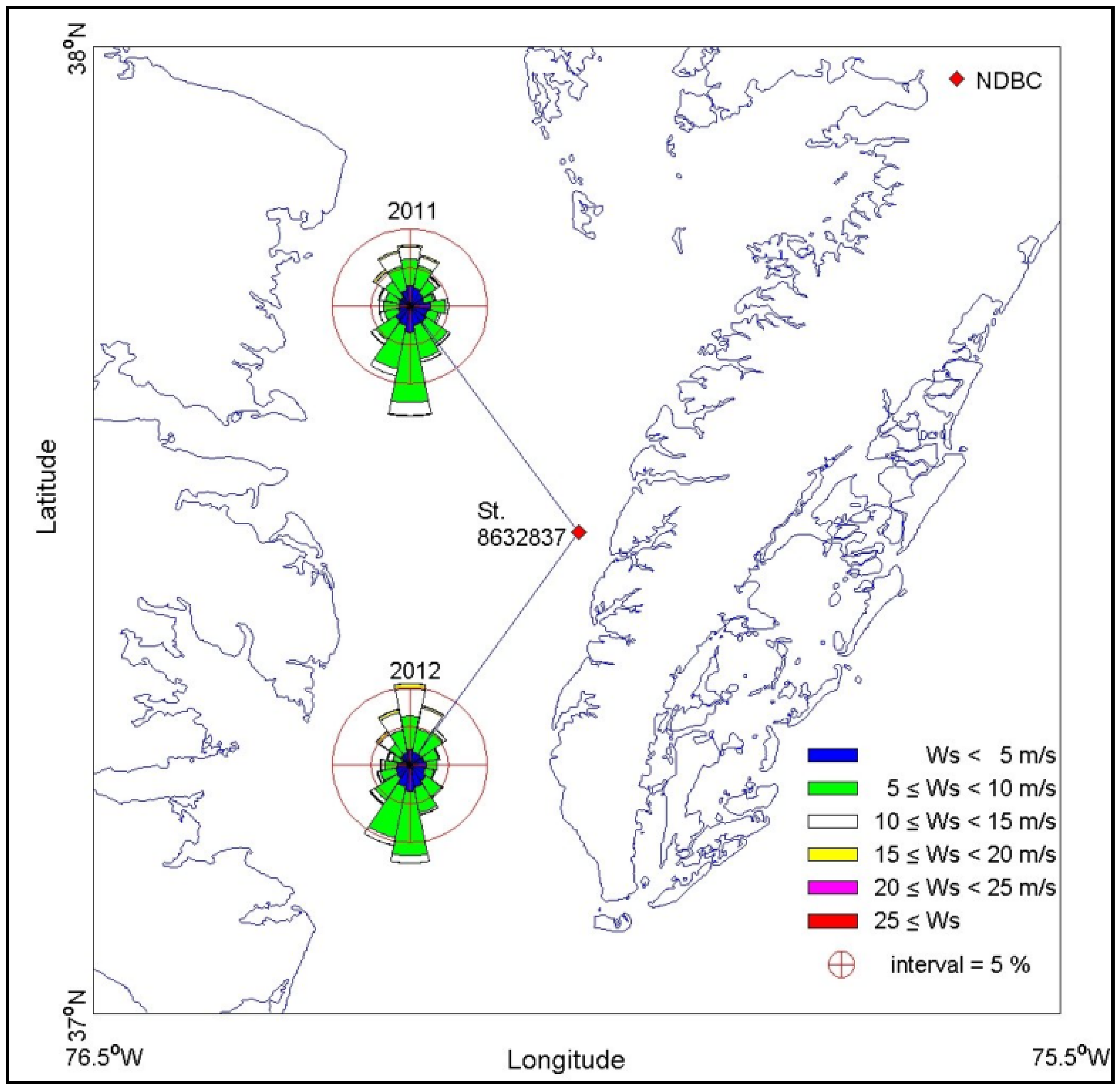
Environmental forces that normally impact the western entrance of Tangier Island boat canal are wind-waves, currents, and water levels. These natural forcings consist of metocean events including summer storms, northeasters, and tropical events, which can impact the Chesapeake Bay and reach Tangier Island from different directions. Seasonal wind patterns vary over the bay. In the winter, the dominant winds are from the north and northwest; they are from the southwest in the summer, with local breezing shifting the wind direction on a daily basis. Larger waves generally occur during northeasters and tropical storms, when high winds blow across the bay.
The west shoreline of Tangier Island is exposed to open water in the lower Bay area, where strong wind can generate large waves.
Figure 3 shows two sample wind roses during for 2011 and 2012 from NOAA station 8632837 (37°32.3′ N, 76°0.9′ E) at Rappahannock Light, VA, approximately 35 km (22 mile) south of Tangier Island in the lower Bay. Winds stronger than 10 m/s (~20 kt) mostly follow a longer fetch along the north–south direction in the Bay. During northeasters with sustained winds of 15 to 20 m/s (30 to 40 kt), local wave heights ranging from 1.5 to 2.5 m (5 to 8 ft) can be expected along the west side of Tangier Island.
Figure 3.
Wind roses for year 2011 and 2012 at NOAA Station 8632837.
Figure 3.
Wind roses for year 2011 and 2012 at NOAA Station 8632837.
Water level fluctuations in the Chesapeake Bay are dominated by oceanic tides interacting with the Bay. Tides at Tangier Island are semi-diurnal, with a 0.6-m mean tidal range. Abnormal water levels or storm surge can occur during tropical events. In the lower Chesapeake Bay, storm surges above the mean water level for 50-year and 100-year recurrence intervals are estimated at 1.5 m and 1.8 m (5 and 6 ft), respectively [
1]. The relative sea level rise estimate due to absolute sea level change and land subsidence in the Chesapeake Bay ranges between 3 and 6 mm/year [
1].
Historically, the Chesapeake Bay froze more often during the 19th and early 20th centuries, but rarely in the last two decades as a result of regional warming, at approximately +1 °C (+2 °F) per decade. The lower Bay may briefly become covered by thinner ice during a severe winter season. The Bay icing is not considered in the present study.
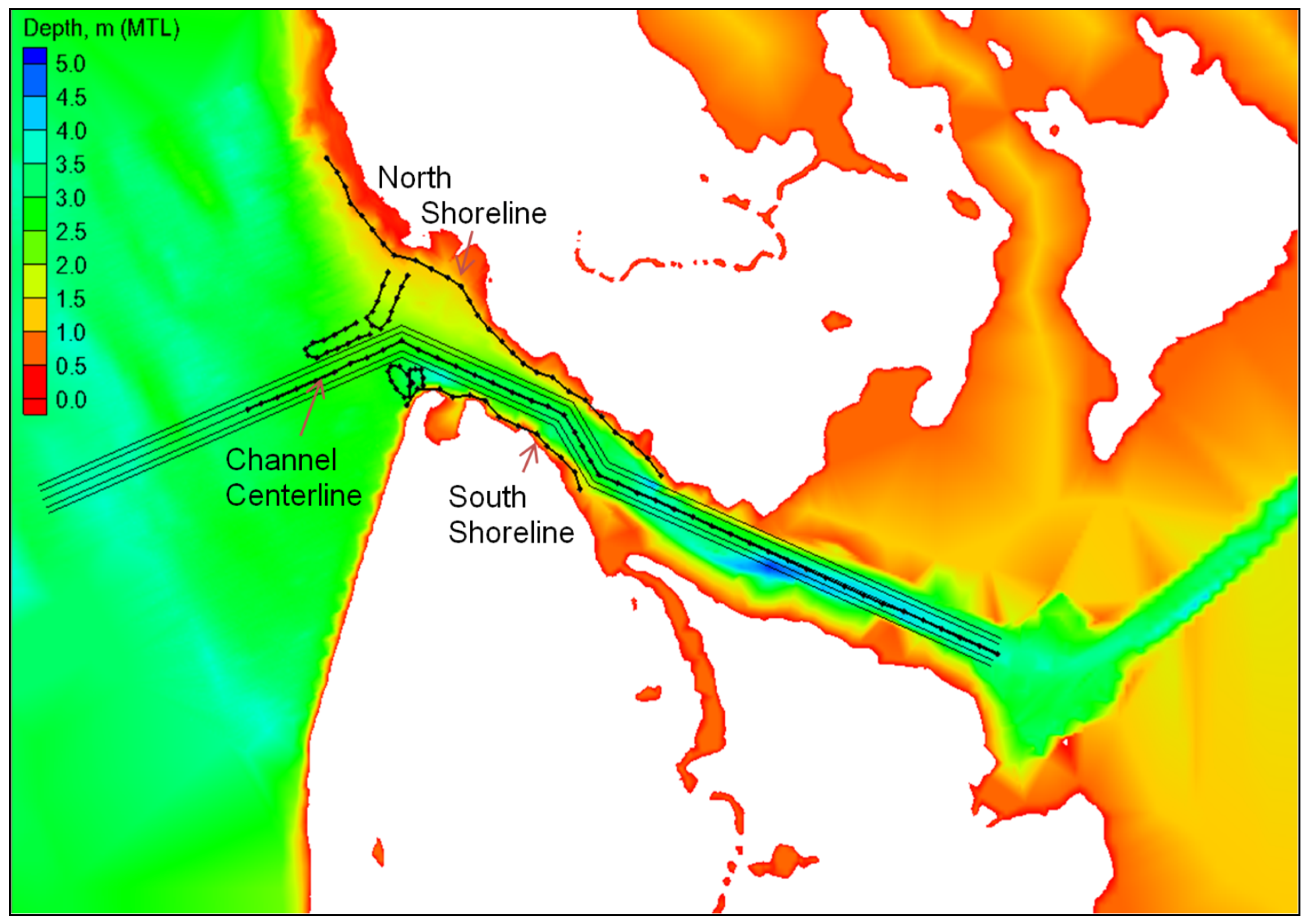
3. Structural Alternatives
The primary area of interest in this modeling study is the west channel section of the Tangier Island boat canal shown in
Figure 4. This narrow canal is the only navigation route that cuts through the middle of Tangier Island and connects the east and west sides of the island. The average west channel base width is 18.3 m (60 ft), the top width is 30.5 m (100 ft), and the channel depth varies from 2.3 to 4 m (7.5 to 13 ft). The narrowest cross section (bank-to-bank) is 70 m (230 ft).
Figure 4.
Western part of Tangier Island boat canal.
Figure 4.
Western part of Tangier Island boat canal.
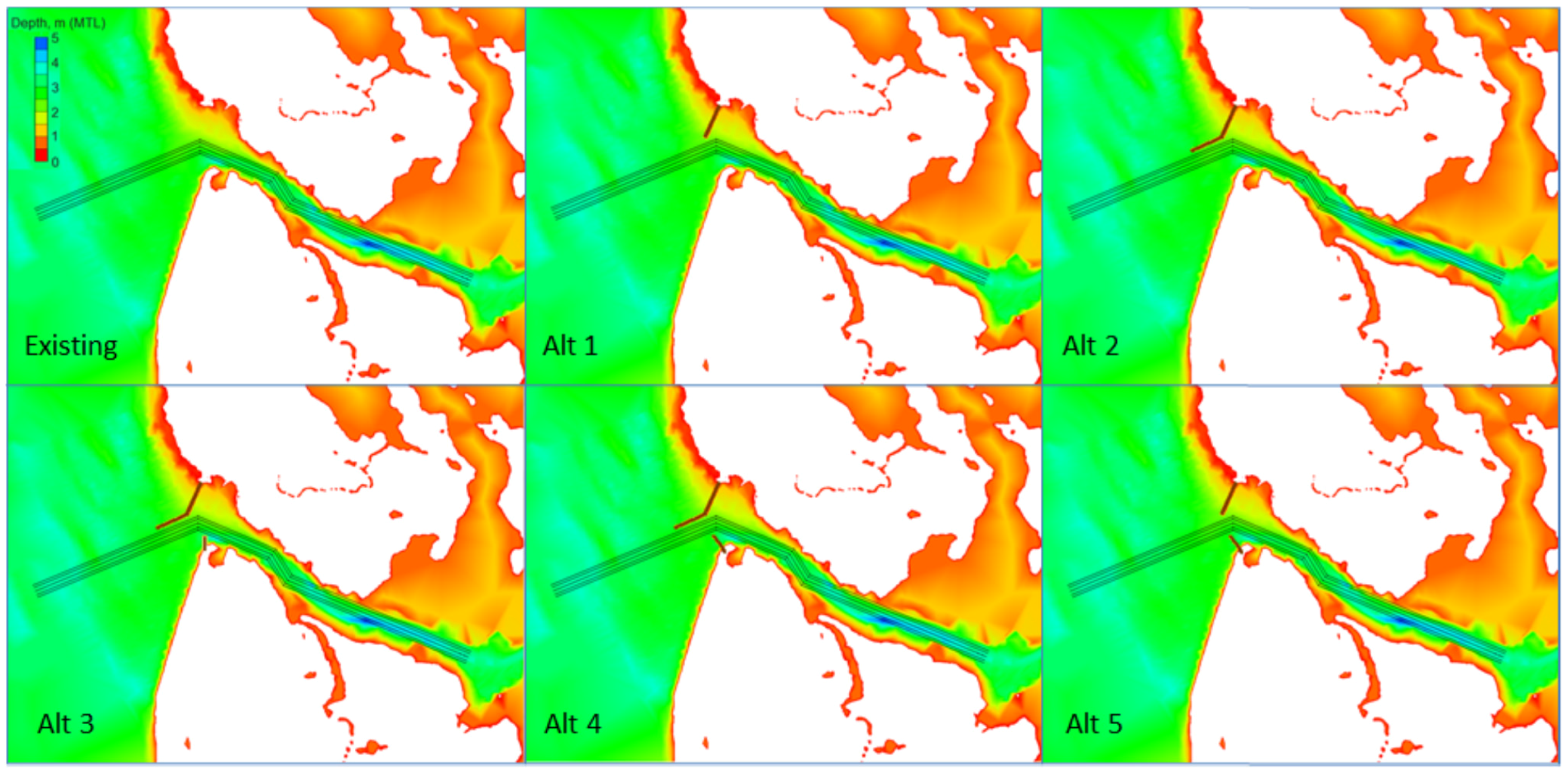
Five structural alternatives with a north jetty connecting to the north shoreline were evaluated, where the north jetty is either a straight or a dogleg structure. Due to cost constraints, the total length of the north jetty is limited to 200 m (650 ft). Alternatives 1 and 2 consider a north jetty of different length. The north jetty is positioned as close to the channel as possible at a safe (for navigation) distance of 50 m to 100 m (164 ft to 328 ft) from the channel edges. Alternatives 3, 4, and 5 include an additional short spur attaching to the south shoreline.
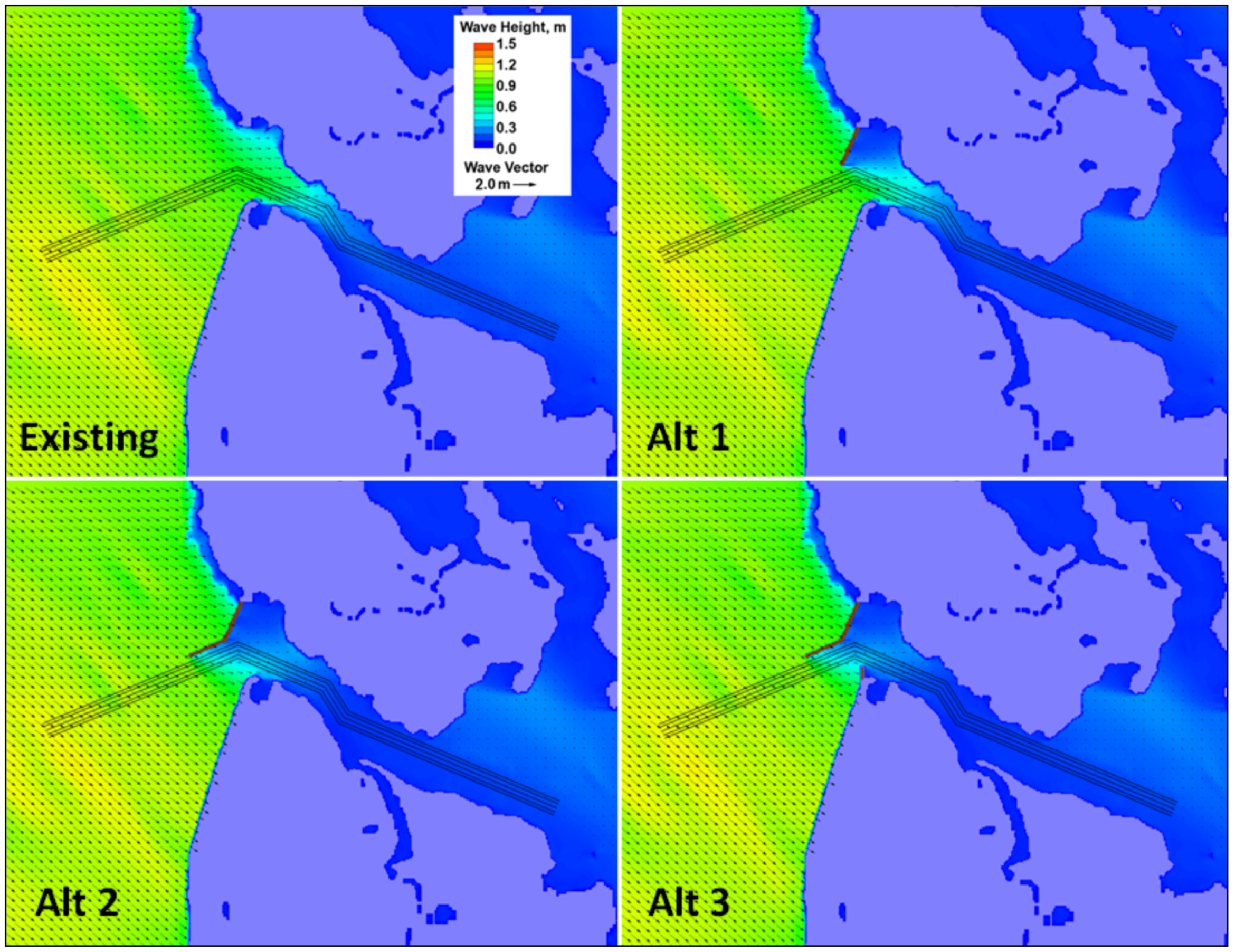
Figure 5 shows depth color contour maps for the existing western entrance channel (channel position and centerline in black lines) and structural features considered in Alternatives 1 to 5 (Alts 1 to 5). In all five alternatives, both jetty and spur structures have a crest elevation of 1 m (3.3 ft) above MTL (roughly the same as MSL) and crest width of 4 m (13 ft). The selection of jetty/spur crest elevation and crest width is based on the cost-to-benefit ratio and federal funding available for construction of structures in the project. The crest and width of proposed jetty/spur structures may be raised and expanded in the future if a higher crest elevation is required. Alt 1 has a straight north jetty 85 m (280 ft) long that is normal to the north shoreline. Alt 2 has a dogleg north jetty 170 m (560 ft) long with a bayward segment 85 m (280 ft) long that is parallel to the entrance channel. Alt 3 has the same dogleg north jetty as in Alt 2 and a short south spur 25 m (82 ft) long that points north (towards the channel). Alt 4 has the same dogleg north jetty as in Alt 2 and a south spur 25 m (82 ft) long directed towards the northwest (normal to south shoreline). Alt 5 has a straight north jetty identical to Alt 1 and a south spur identical to Alt 4. In addition to guiding the tidal flow along the navigation channel, the second purpose of the north jetty is to protect the shoreline east of the north jetty from wave action. The primary purpose of the south spur is to stabilize the shoreline south of the spur and reduce wave penetration into the western entrance channel.
Table 1 presents a summary of existing channel and structural features for the five alternatives.
Figure 5.
Depth color contours of the existing western entrance channel and Alts 1 to 5.
Figure 5.
Depth color contours of the existing western entrance channel and Alts 1 to 5.
Table 1.
Structural features of alternatives.
Table 1.
Structural features of alternatives.
| Alt | Straight North Jetty (85 m Long) | Dogleg North Jetty (170 m Long) | South Spur (25 m Long) Toward Channel | South Spur (25 m long) Normal to Shoreline |
|---|
| 1 | X | | | |
| 2 | | X | | |
| 3 | | X | X | |
| 4 | | X | | X |
| 5 | X | | | X |
4. Numerical Modeling Approach
The Coastal Modeling System (CMS) was used to calculate waves, currents, sediment transport, and morphology change [
2]. It is an integrated modeling system that consists of a steady-state spectral wave model (CMS-Wave) and a two-dimensional, time-dependent circulation model (CMS-Flow), which includes sediment transport and bed change capabilities. The CMS uses the Surface-water Modeling System (SMS) interface for grid generation, model setup, and post-processing [
3].
The CMS models can run on a grid with variable rectangular cells. To save computational time, large cells can be used in large-area applications away from the area of interest while fine-grid resolution is used in the area of interest. The CMS can also run on nested grids that include many large and small grids [
4]. The most commonly applied grid nesting involves two model grids: a large grid (parent grid) and a small grid (child grid). The application of grid nesting can dramatically reduce the computational time as compared to a large grid with fine resolution for the entire model domain. A parent grid may be used to simulate regional processes such as wave generation and propagation in a large domain. A child grid can resolve more complex bathymetry and shoreline geometry in a smaller area for more accurate modeling of nearshore wave processes. Water levels and currents calculated from the parent grid are interpolated to the child grid boundaries. Wave spectra calculated from the parent grid are saved at selected locations along the offshore boundary of the child grid. Conventionally, it suffices to save a single-location spectrum from the large-domain parent grid for wave input and apply it to the entire sea boundary of a comparatively much smaller domain child grid. For a more inhomogeneous wave field, multiple locations of wave spectra may be saved from the parent grid and interpolated for more realistic wave forcing along the seaward boundary of the child grid. The main goal of grid nesting is to minimize computational time while not sacrificing modeling accuracy.
The CMS has been applied in many coastal wave, circulation, and sediment transport studies including open coasts, inlets, bays, estuaries, and lakes [
5]. Most recent bay applications include modeling waves, flow, and sediment transport of Braddock Bay in Lake Ontario [
6], and Matagorda Bay and Galveston Bay in Texas [
7,
8].
The CMS uses physics-based theories to calculate wave generation, growth, and dissipation under variable wind/pressure fields in a bay-ocean system and, therefore, can simulate large-scale storm and hurricane events [
9,
10,
11,
12,
13,
14]. The use of the CMS in wave modeling is more realistic for bay applications and more accurate than classical fetch-based empirical curves as the wind wave generation and growth are strongly affected by the complex of bay geometry and varying bathymetry [
15,
16]. This is particularly true in the Chesapeake Bay because many river tributaries, navigation channels, shoals, islands, and peninsulas coexist in the Bay. The long narrow lake basin with the broader lower bay connecting to the Atlantic Ocean causes more complexity of wave action and flow circulation in the Chesapeake Bay. Because the western channel of Tangier Island is exposed to open water in the lower Bay, strong winds from the northwest and southwest quadrants can generate large waves in the area. During a tropical storm, Tangier Island may be threatened by high water as low atmospheric pressure and strong wind can trap water against the higher ground barriers and land to the east and north of the island.
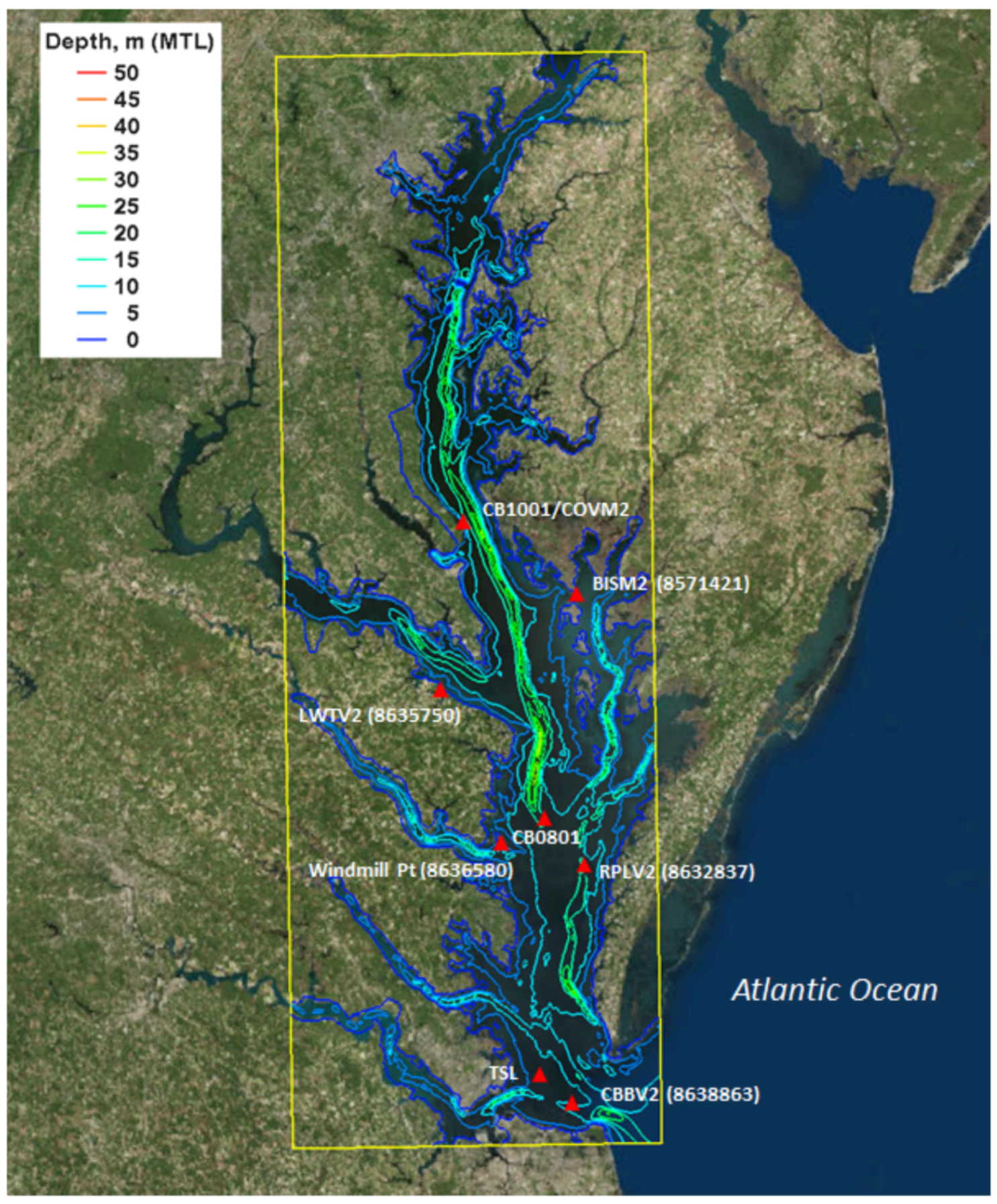
Figure 6 shows the CMS modeling domain for the Chesapeake Bay region and corresponding depth contours. This bay-wide large grid domain, approximately 100 km by 300 km (60 miles by 180 miles), is referred to as the regional grid (parent grid), which has a constant grid cell size of 500 m by 500 m (1600 ft by 1600 ft). The depths in this grid vary from 0 to 45 m (0 to 150 ft). The CMS modeling includes a second domain, referred to as the local grid (child grid) for Tangier Island, which is shown in
Figure 1 and
Figure 2. This grid has a finer resolution to represent details of Tangier Island shorelines and bathymetry. The domain of the child grid is approximately 5 km by 7 km (3 miles by 4.4 miles), with the local grid cell size varying from 3 m to 50 m (10 ft to 160 ft).
Figure 6.
NOAA and VIMS coastal stations (red triangle) and CMS depth contours (m, MTL) for the CMS Chesapeake Bay regional grid domain (yellow box).
Figure 6.
NOAA and VIMS coastal stations (red triangle) and CMS depth contours (m, MTL) for the CMS Chesapeake Bay regional grid domain (yellow box).
4.1. Model Calibration
The calibration of the CMS was conducted separately for CMS-Wave and CMS-Flow in the Chesapeake Bay regional grid. CMS-Wave was calibrated using wave spectral data collected at Thimble Shoal Light (TSL) gauge (see
Figure 6), maintained by the Virginia Institute of Marine Science (VIMS) from 1988 to 1995 [
16,
17,
18].
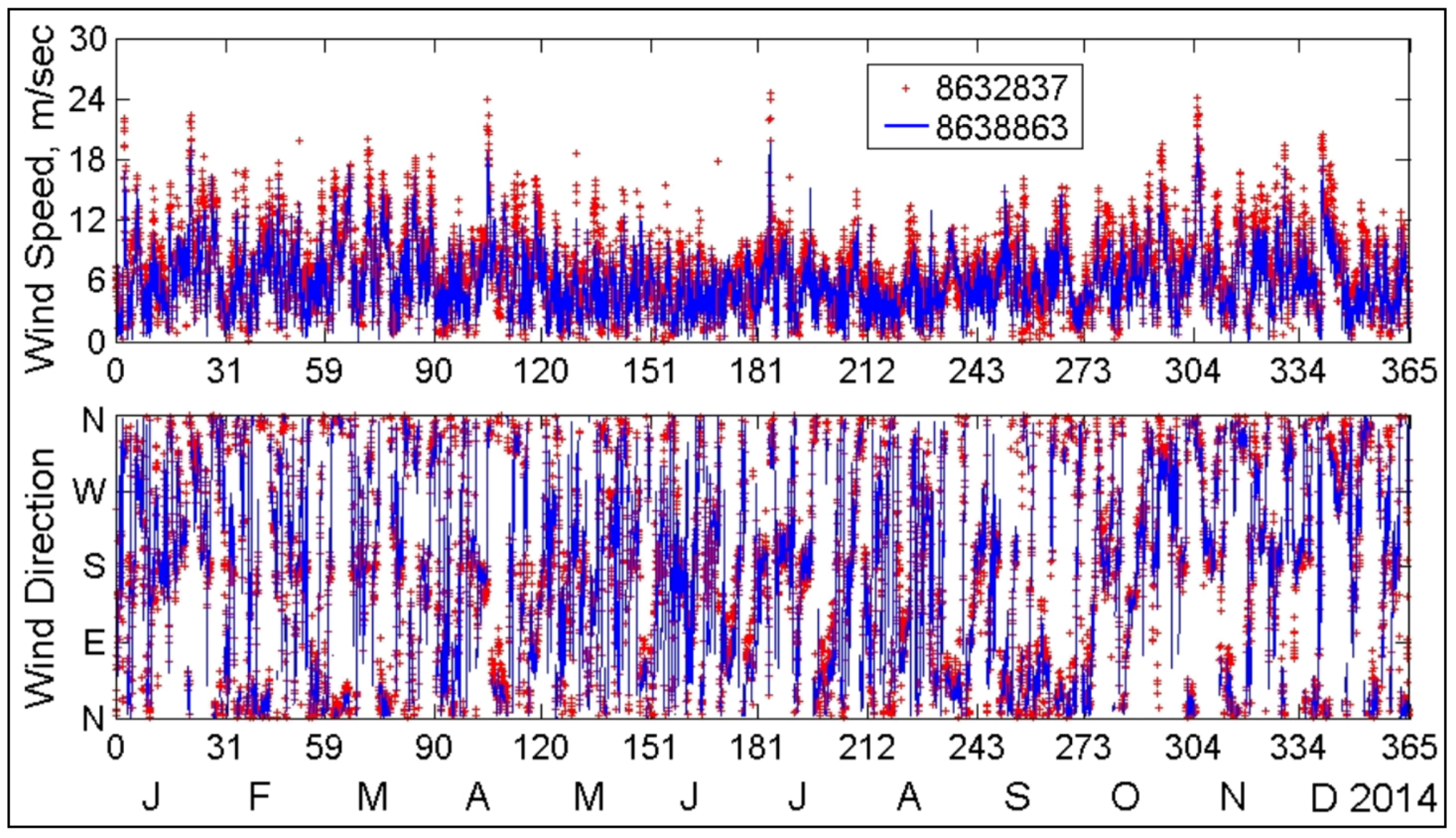
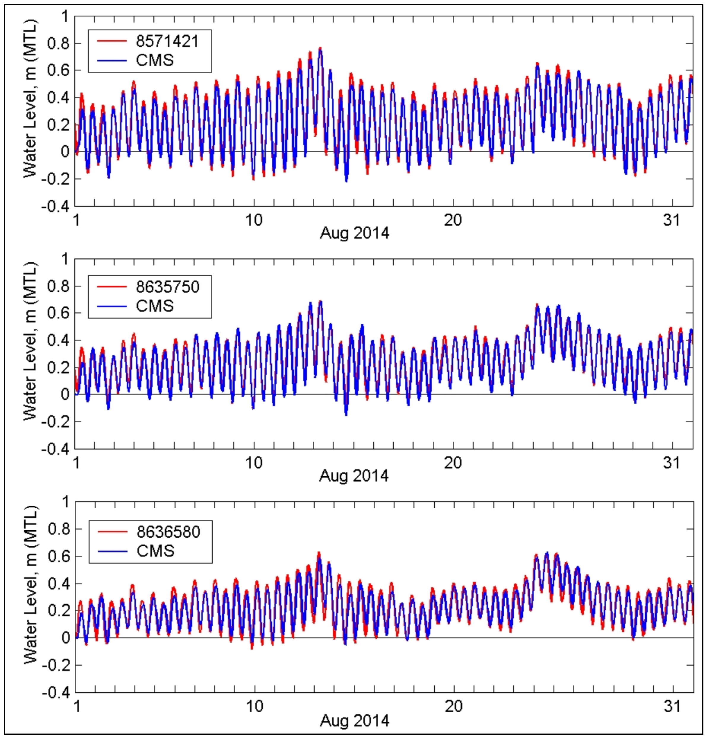
The calibration of CMS-Flow was conducted for August 2014. CMS-Flow was forced by hourly water level data, collected from NOAA Coastal Station 8638863 (Chesapeake Bay Bridge Tunnel, VA, USA), along the lower bay entrance boundary for flow exchange with the Atlantic Ocean. Atmospheric input to CMS-Flow was based on hourly wind data collected at NOAA Station 8632837 (Rappahannock Light, VA, USA). August 2014 was selected in CMS-Flow calibration because the wind speed for this month was on average the lowest during the year and so the effect of wind on tidal hydrodynamics is small for the calibration.
Figure 7 shows thr wind data collected at NOAA 8632837 and 8638863 in 2014 [
19]. A hydro time step of 15 s and spatially constant Manning coefficient of 0.02 were used in the model calibration.
Figure 8 shows the model-data comparison water levels at NOAA Stations 8571421 (Bishops Head, MD, USA), 8635750 (Lewisetta, VA, USA), and 8636580 (Windmill Point, VA, USA). Model water levels and data are correlated well. Correlation coefficients between model water levels and data at Stations 8571421, 8635750, and 8636580 are equal to 0.98, 0.97, and 0.93, respectively.
Figure 7.
Wind measurements at Rappahannock Light, VA (8632837) and Chesapeake Bay Bridge Tunnel, VA (8638863) for 2014.
Figure 7.
Wind measurements at Rappahannock Light, VA (8632837) and Chesapeake Bay Bridge Tunnel, VA (8638863) for 2014.
Figure 8.
Model and measured water levels at Bishops Head, MD (8571421), Lewisetta, VA (8635750), and Windmill Point, VA (8636580) for August 2014.
Figure 8.
Model and measured water levels at Bishops Head, MD (8571421), Lewisetta, VA (8635750), and Windmill Point, VA (8636580) for August 2014.
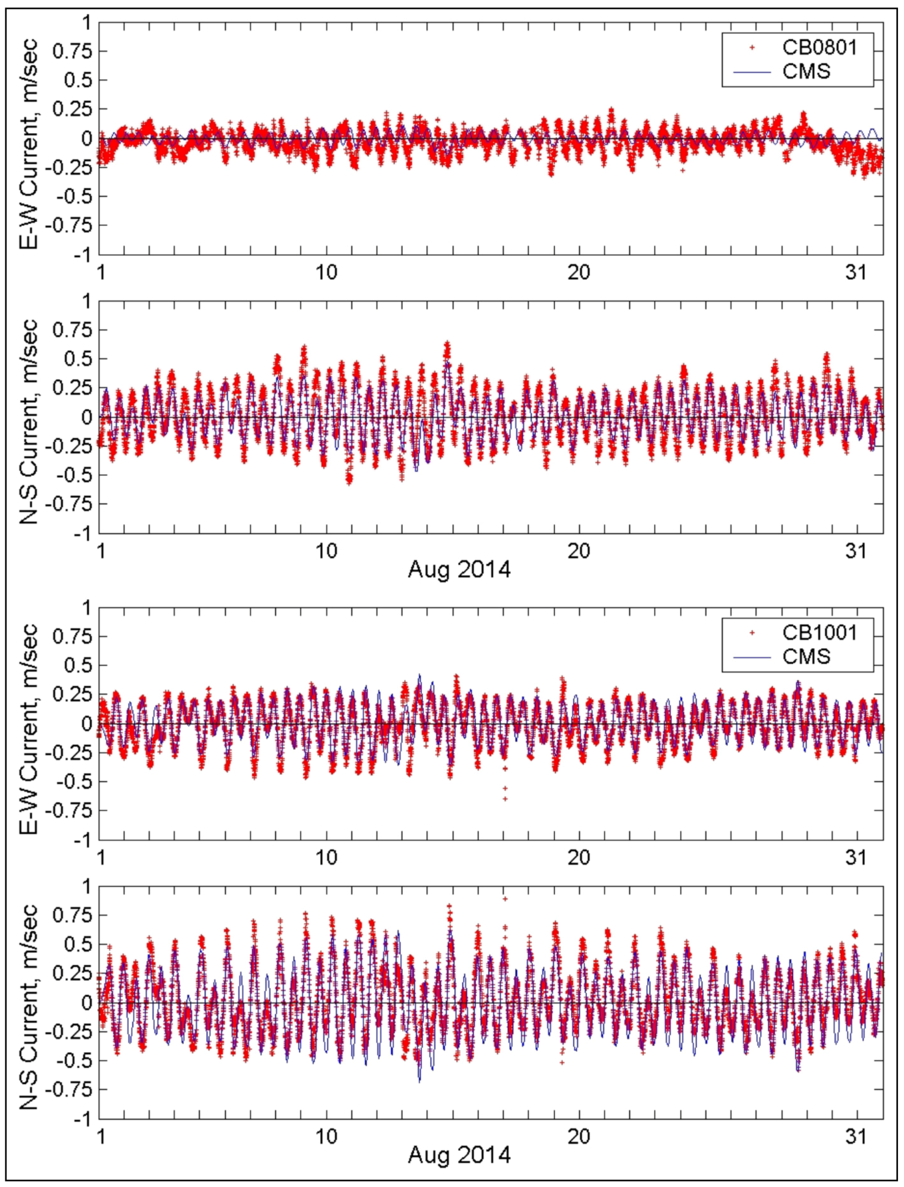
Surface current measurements were available in the mid- and south Chesapeake Bay during 2014 from NOAA Stations CB0801 (Rappahannock Shoal Channel, VA, USA) and CB1001 (Cove Point LNG Pier, MD, USA).
Figure 9 compares easting and northing current components calculated by CMS-Flow with data collected at CB0801 and CB1001. The positive current speed component along the East–West (E–W) line is directed to the east, and the positive component along the North–South (N–S) line is directed to the north. Because model currents are depth-averaged and the data are for surface currents, the magnitude of the model currents is generally smaller than in the data. Correlation coefficients between model current E–W components and data at CB0801 and CB1001 are equal to 0.27 and 0.88, respectively. Lesser correlation between E–W components and the data at CB0801 is likely due to more wind–wave interactions over weaker E–W components which are not simulated in the calibration. Correlation coefficients between model current N–S components and data at both CB0801 and CB1001 are equal to 0.89.
Figure 9.
Comparison of calculated depth-averaged current components and measured surface current data at NOAA Stations CB0801 and CB1001 for August 2014.4.2.
Figure 9.
Comparison of calculated depth-averaged current components and measured surface current data at NOAA Stations CB0801 and CB1001 for August 2014.4.2.
4.2. Forcing Conditions
After model calibration, the modeling focused on structural design estimates for a 50-year return period for design storm conditions and a historical hurricane. For the 50-year design storm conditions, a constant wind speed of 20 m/s (40 kt) was selected based on a previous study by Basco and Shin (1993) from analysis of 1945–1983 storms at Patuxent Naval Air Station. The storms included both tropical events and northeasters. In the present study, wave generation was simulated for nine constant wind directions covering a westerly half-plane sector from north to south. These nine directions, each covering a 22.5-deg angle, present the design wind from the N, NNW, NW, WNW, W, WSW, SW, SSW, and S directions. Model simulations were conducted for two different water levels representing the observed mean tide level (WL = 0 m) and high water level (WL = 1.5 m or 5 ft) from nearby NOAA coastal stations located in the mid- and lower bay (
Figure 6).
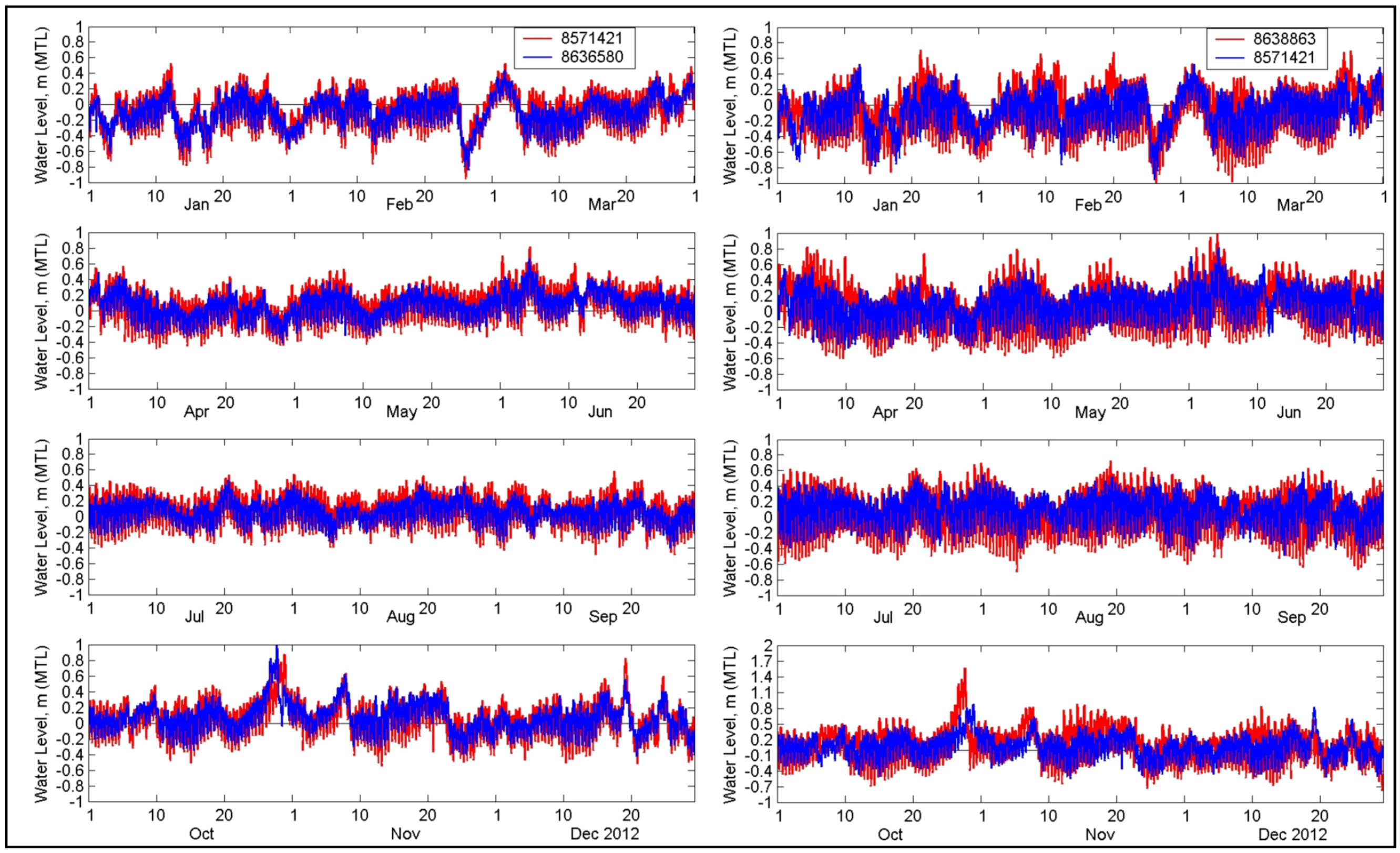
Figure 10 shows the example of the water level measurements for year 2012 recorded at three NOAA Stations: 8571421 (Bishops Head, MD), 8636580 (Windmill Point, VA), and 8638863 (Bay Bridge Tunnel, VA). The maximum water level observed at Bay Bridge Tunnel Station was 1.5 m (5 ft), MTL, during Hurricane Sandy.
Table 2 lists the 50-year design wind conditions with wind speed of 20 m/s and nine wind directions for two water levels (WL) of 0 and 1.5 m (5 ft).
Table 2 also lists the approximate fetch length corresponding to each of the nine wind directions. In general, the wind over longer fetch generates greater wave height at the downwind end, although in reality this also depends on the water depth variation along the fetch and wave refraction over shallower areas before waves reach the oblique shoreline.
Figure 10.
Water levels at Bishops Head (Station 8571421), Windmill Point (8636580), and Bay Bridge Tunnel (8638863) for 2012.
Figure 10.
Water levels at Bishops Head (Station 8571421), Windmill Point (8636580), and Bay Bridge Tunnel (8638863) for 2012.
Table 2.
Design wind and water level conditions for a 50-year return period northeaster storm.
Table 2.
Design wind and water level conditions for a 50-year return period northeaster storm.
| Wind Dir (deg) * | N (0) | NNW (337.5) | NW (315) | WNW (292.5) | W (270) | WSW (247.5) | SW (225) | SSW (202.5) | S (180) |
|---|
| Fetch ** (km) | 30 | 55 | 70 | 25 | 20 | 25 | 30 | 45 | 100 |
| Wind Speed | 20 m/s |
| Mean Tide Level | WL = 0 m |
| Mean High Water | WL = 1.5 m |
Two water levels (WL) were used in wave simulations for the 50-year design wind conditions: were 0 and 1.5 m (5 ft) with respect to MTL. The WL = 0 m represented the mean water level corresponding to non-tropical storm (e.g., northeasters) design wind conditions, and WL = 1.5 m corresponded to the maximum storm surge for tropical storm (or hurricanes) design wind conditions. Since there is no water level measurement at Tangier Island, the selection of maximum storm surge during a hurricane is based on water level data collected in the last 50 years (after 1965) from three nearby NOAA coastal stations at Bishop Heads (Station ID 8571421), Lewisetta (8635750), and Windmill Point (8636580). These stations show that the maximum storm surge is approximately 1.5 m during Hurricanes Isabel (2003) and Sandy (2012) [
13,
20]. Therefore, WL = 1.5 m MTL was used as the maximum storm surge for the tropical storm in the 50-year design wind condition.
For a 50-year tropical event, Hurricane Isabel (September 2003) was selected and simulated in the entire Bay [
20,
21]. The strong east-to-west winds associated with Hurricane Isabel produced higher water levels along the west as well as the south side of the bay and a relatively lower water level along the east side of the bay.
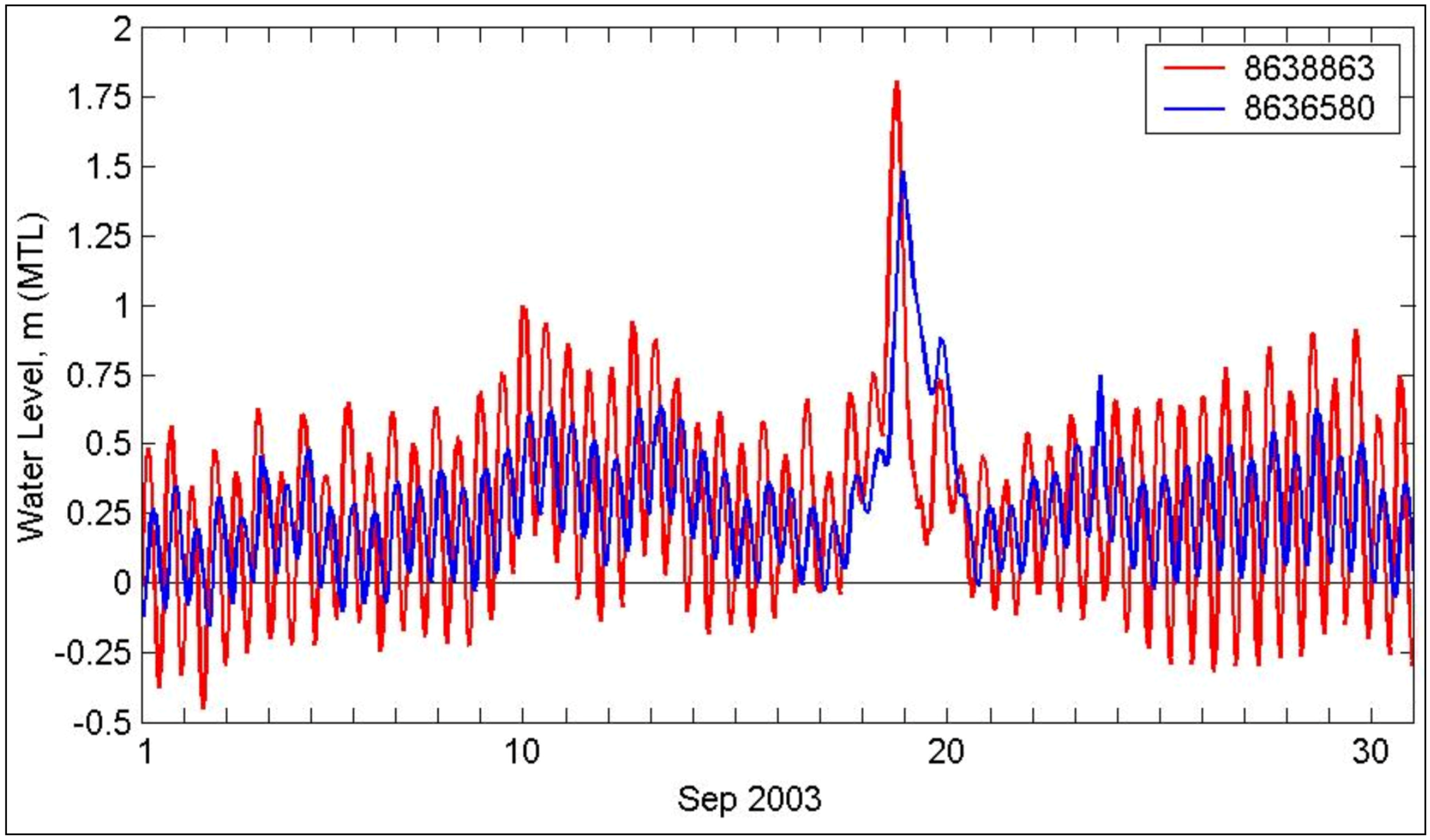
Figure 11 shows the examples of water level measurements from Bay Bridge Tunnel (8638863) and Windmill Point, VA (8636580) during Isabel in September 2003. The maximum water levels observed at Stations 8638863 and 8636580 were 1.87 m (6.1 ft) and 1.44 m (4.7 ft) MTL, respectively.
4.3. Design Wind and Water Level Simulations
Design wind and wave simulations were performed for nine wind directions and two water levels, 0 and 1.5 m (0 and 5 ft) MTL, listed in
Table 2. The design wind conditions, representing the 50-year return period, were used for the existing western channel and Alts 1 to 5 (
Figure 5). The 50-year wind condition was based on a previous study by Basco and Shin [
22]. The simulations were first conducted with a regional grid, and results were then used as input in the local Tangier Island grid calculations.
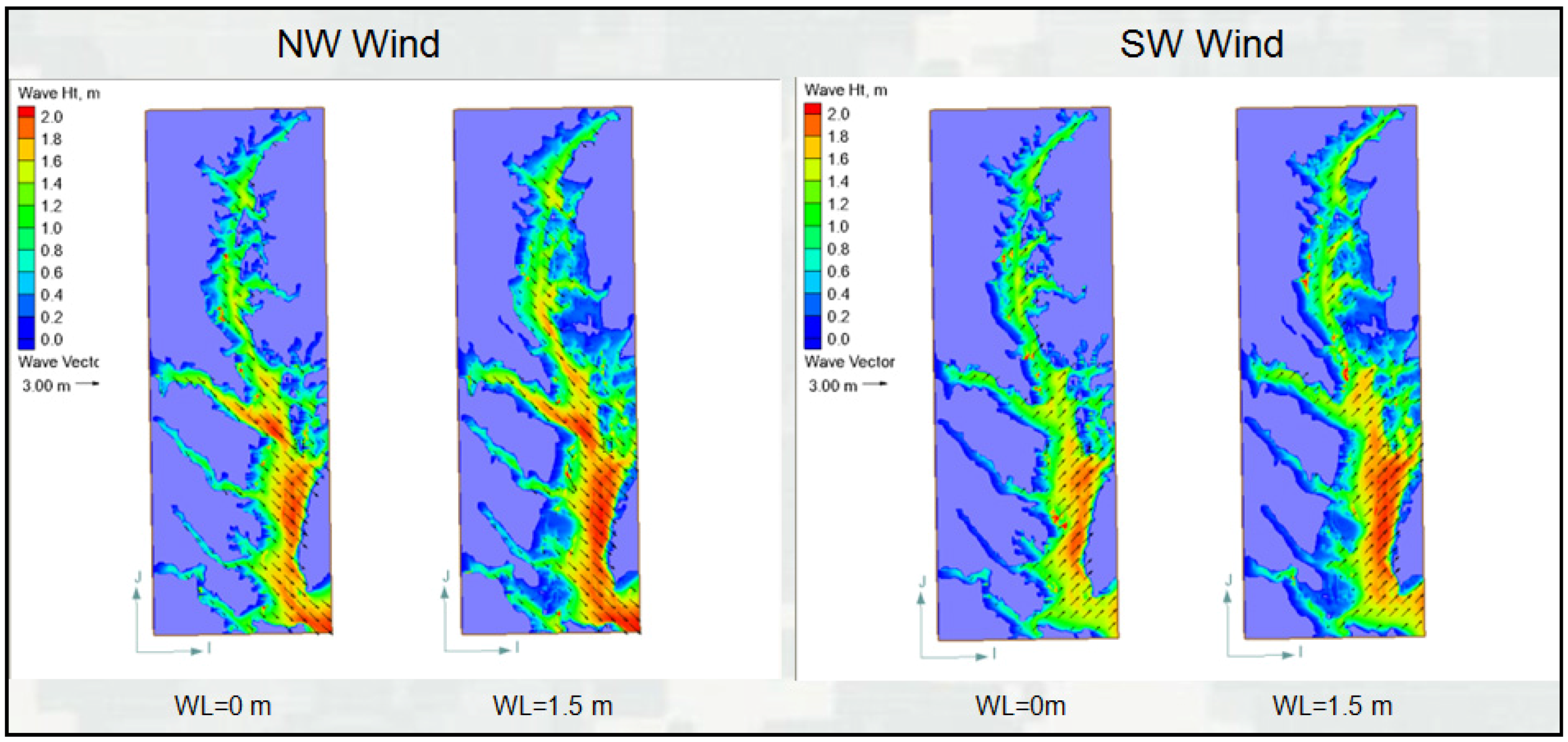
A total of 108 simulations (nine wind conditions, two water levels, and six configurations) were performed to develop spatially varying estimates of the wind waves throughout the Chesapeake Bay. As an example,
Figure 12 shows the bay-wide wave height fields calculated by the CMS for two wind directions from NW and SW (wind speed of 20 m/s or 40 kt) and two water levels of 0 and 1.5 m (5 ft) MTL.
Figure 11.
Water levels at Bay Bridge Tunnel (8638863) and Windmill Point (8636580), VA, for September 2003.
Figure 11.
Water levels at Bay Bridge Tunnel (8638863) and Windmill Point (8636580), VA, for September 2003.
Figure 12.
Calculated wave heights in Chesapeake Bay at two water levels (50-year design winds from NW and SW directions).
Figure 12.
Calculated wave heights in Chesapeake Bay at two water levels (50-year design winds from NW and SW directions).
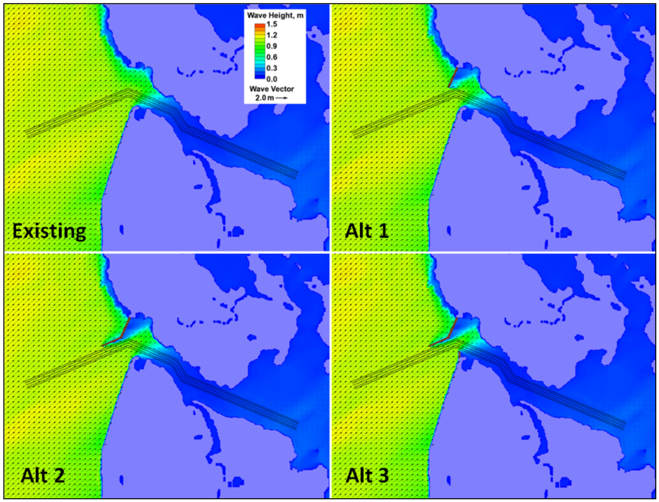
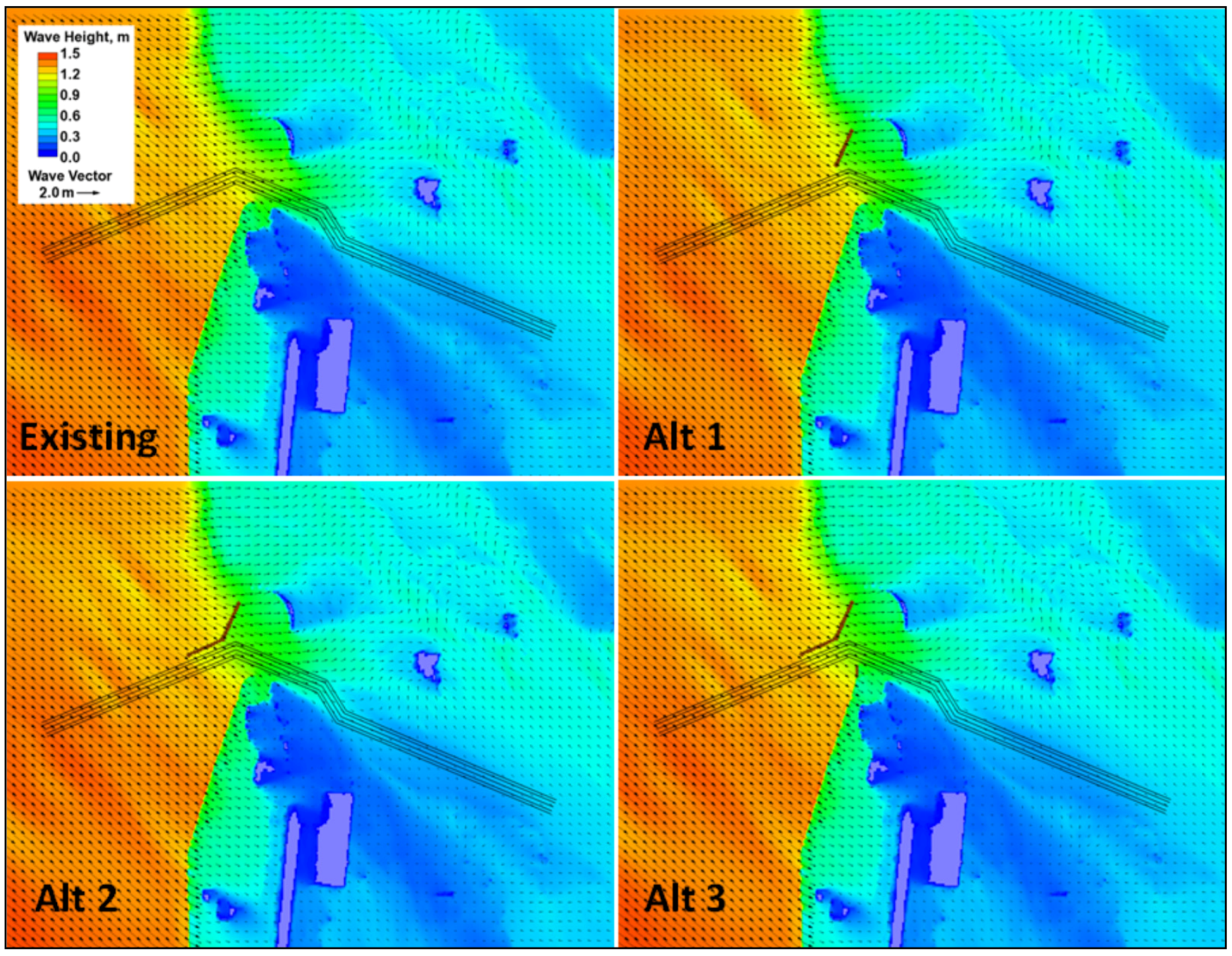
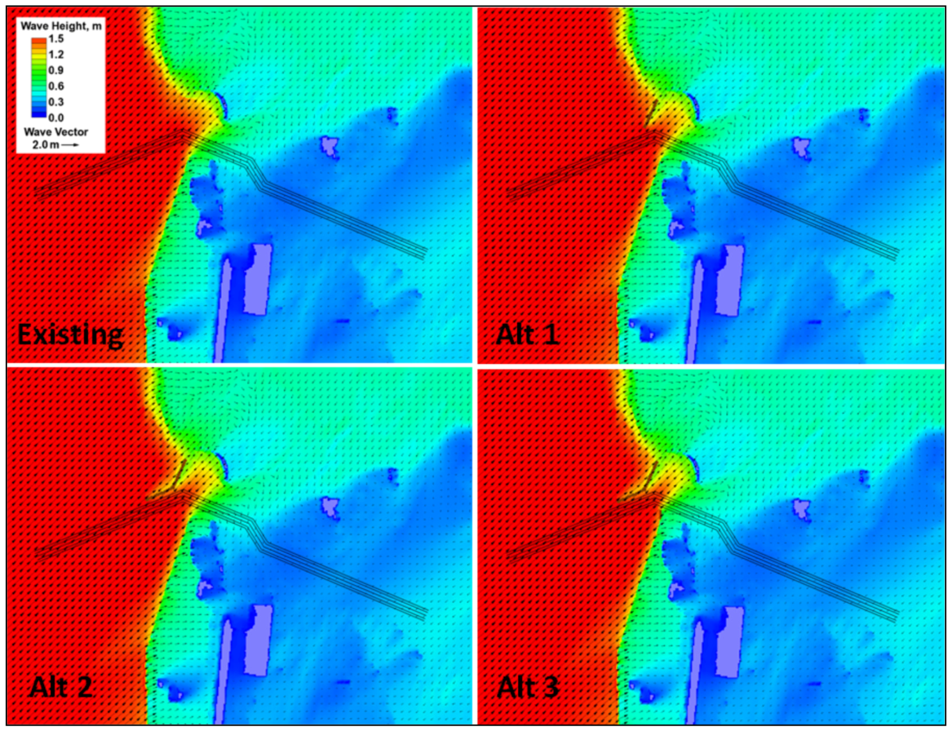
Wave model results from the regional grid (parent grid) for the entire Bay were used as input in the local grid (child grid) to develop the estimates of waves at the project site.
Figure 13,
Figure 14,
Figure 15 and
Figure 16 show contour and vector plots of calculated wave height and direction for Existing, Alts 1, 2, and 3, respectively, for 50-year design wind speed of 20 m/s from NW and SW, and water levels of 0 m and 1.5 m MTL. The extent of wave penetration into the canal, and variation of wave heights along the channel centerline and north and south shorelines are shown in the color-coded plots of wave field in
Figure 13,
Figure 14,
Figure 15 and
Figure 16. It should be noted that because CMS-Wave is a steady-state spectral model, the calculated wave field corresponds to a saturated sea state for each input wind condition. The saturated sea is also known as the developed sea that water surface waves cannot grow more under the specified wind input condition. This is possible in open water under constant wind conditions over a sufficiently long time period. In a limited fetch area (e.g., in a bay or lake) for the same wind conditions, wave generation can reach saturated state in a relatively shorter time. Because the Chesapeake Bay has a limited water body, the saturated sea calculated by the CMS-Wave should provide a good approximation of the design wind conditions. The calculated corresponding wave height is the maximum wave field for the design wind. The wave reduction analysis was performed for all simulations by comparing alternatives to the existing channel along three transact lines along the channel centerline and the north and south shorelines (
Figure 17). Model wave heights were saved at 103 stations along these three transacts for further analysis (
Figure 18).
Figure 13.
Example of model calculated wave heights in the west channel for the 50-year design winds from NW at 0 m water level.
Figure 13.
Example of model calculated wave heights in the west channel for the 50-year design winds from NW at 0 m water level.
Figure 14.
Example of model calculated wave heights in the west channel for the 50-year design winds from SW at 0 m water level.
Figure 14.
Example of model calculated wave heights in the west channel for the 50-year design winds from SW at 0 m water level.
Figure 15.
Example of model calculated wave heights in the west channel for the 50-year design winds from NW at 1.5 m water level.
Figure 15.
Example of model calculated wave heights in the west channel for the 50-year design winds from NW at 1.5 m water level.
Figure 16.
Example of model calculated wave heights in the west channel for the 50-year design winds from SW at 1.5 m water level.
Figure 16.
Example of model calculated wave heights in the west channel for the 50-year design winds from SW at 1.5 m water level.
Figure 17.
Three transects (lines) used to extract model wave heights.
Figure 17.
Three transects (lines) used to extract model wave heights.
Figure 18.
Point locations (stations) used to extract model wave heights.
Figure 18.
Point locations (stations) used to extract model wave heights.
5. Results and Discussion
5.1. Fifty-Year Design Wind Waves
The wave reduction analysis was performed for all simulations by comparing model results for the alternatives to the existing channel.
Figure 19,
Figure 20,
Figure 21,
Figure 22,
Figure 23 and
Figure 24 show these comparisons of wave height variation along the west channel centerline for the NW, W, and SW directions.
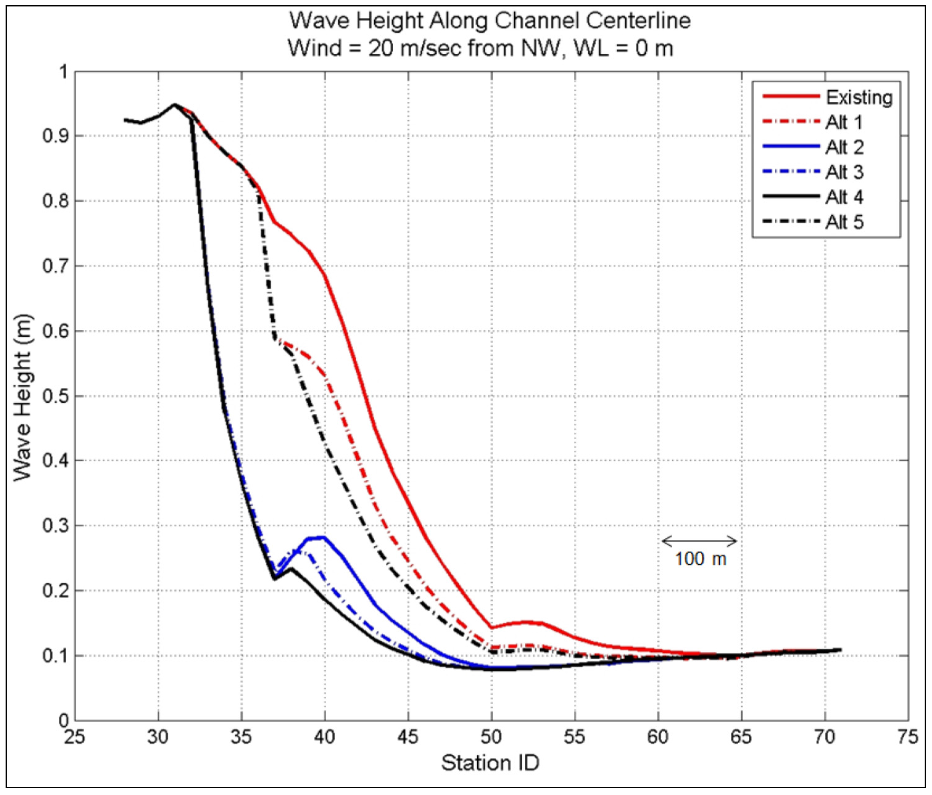
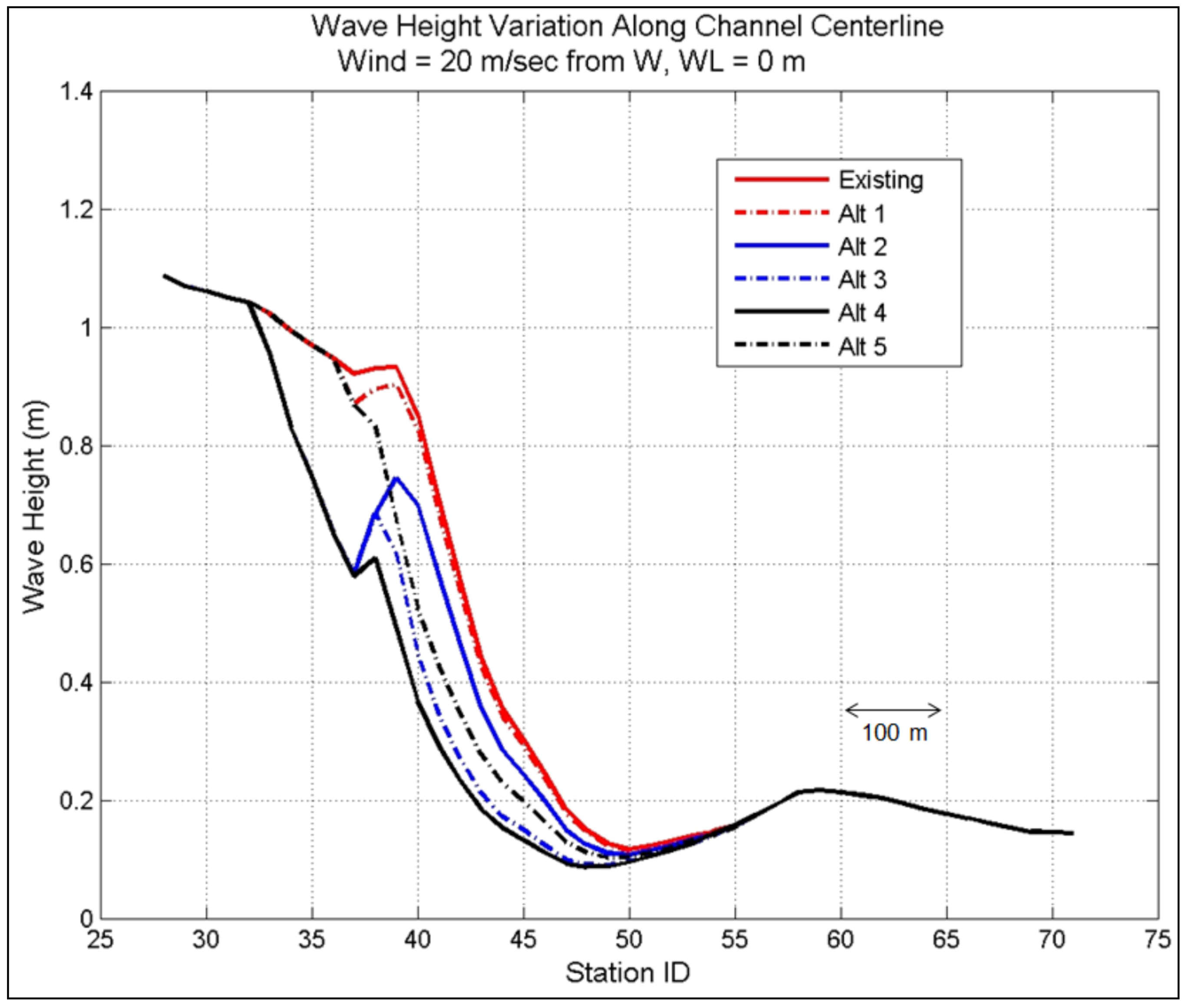
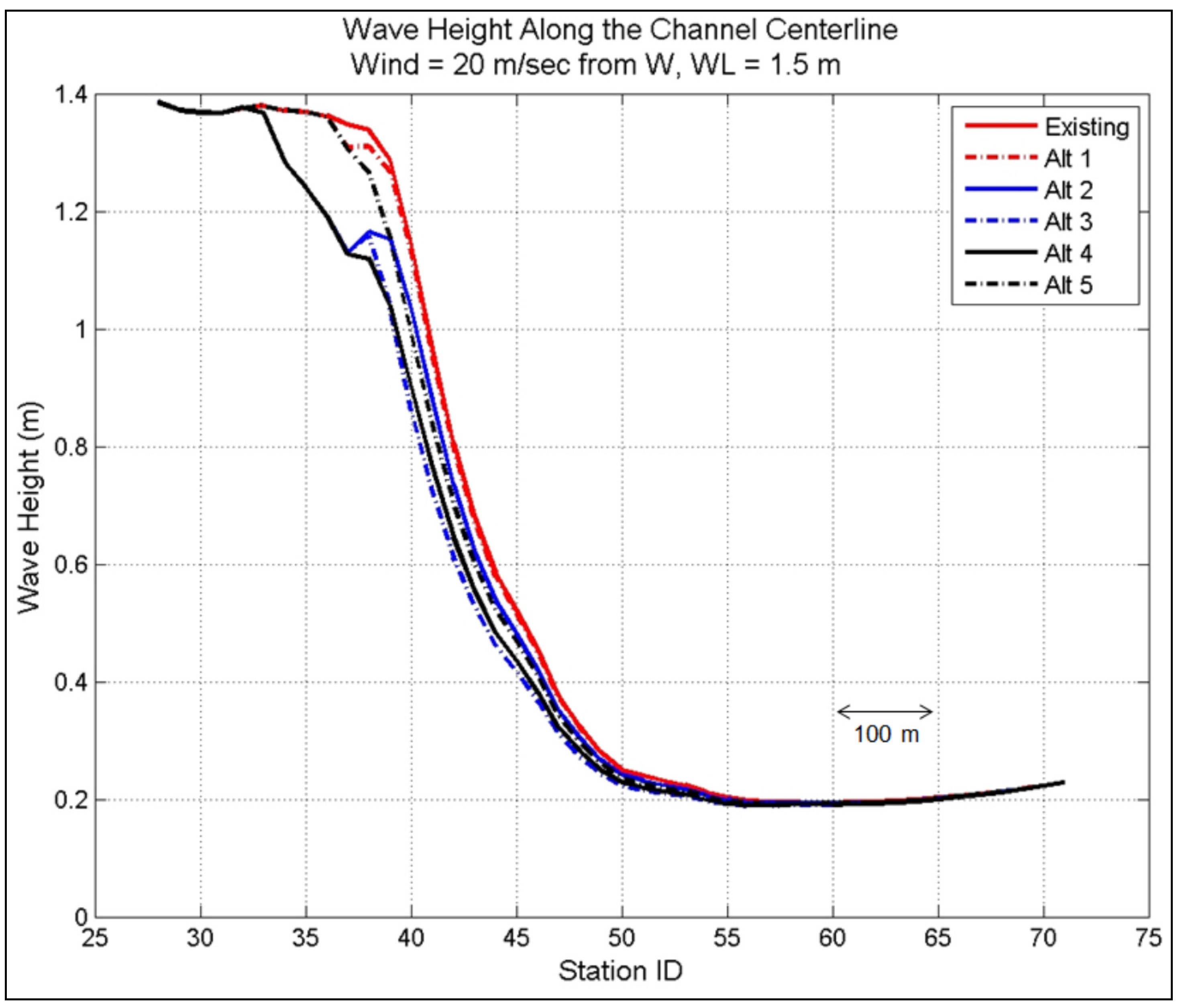
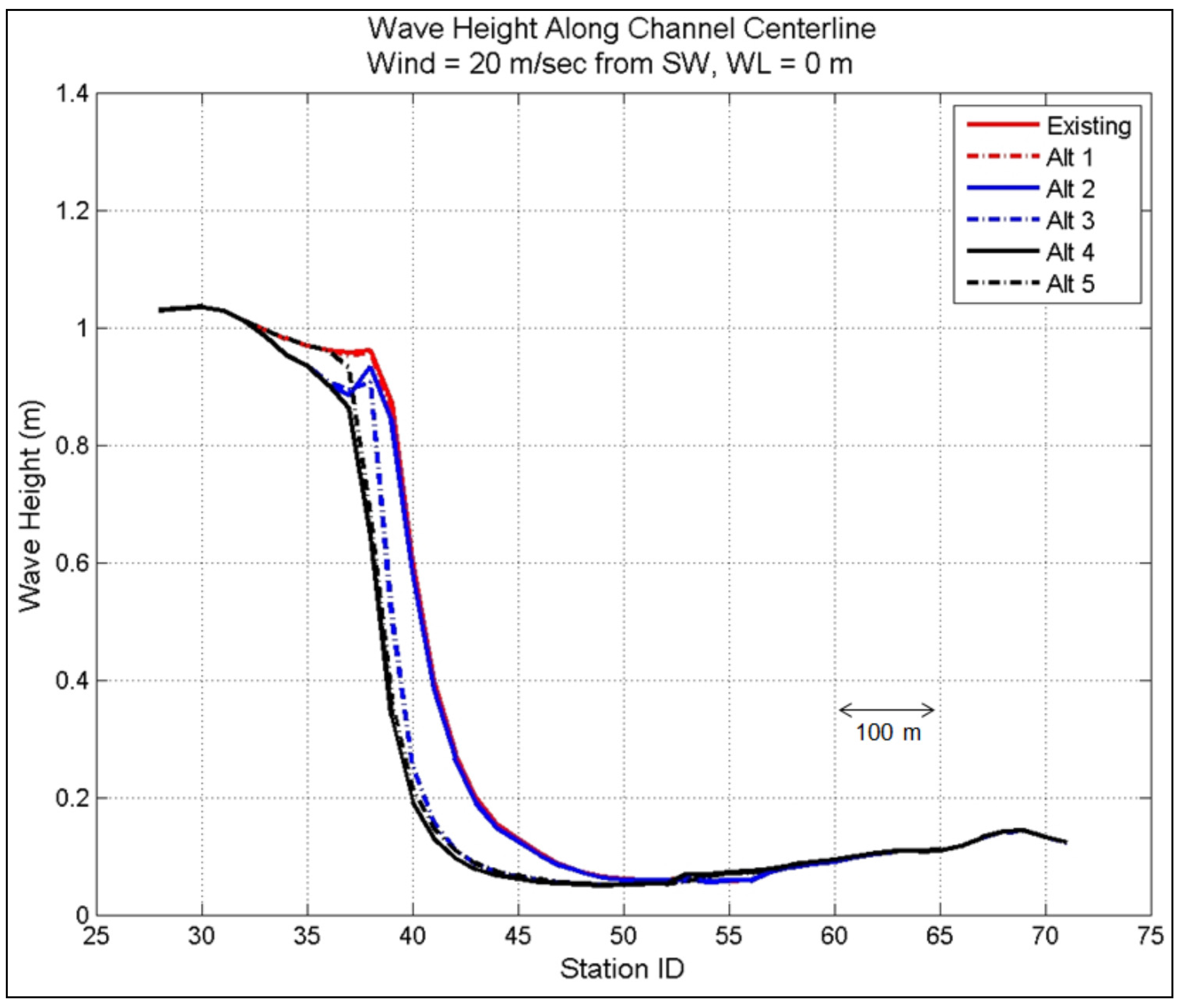
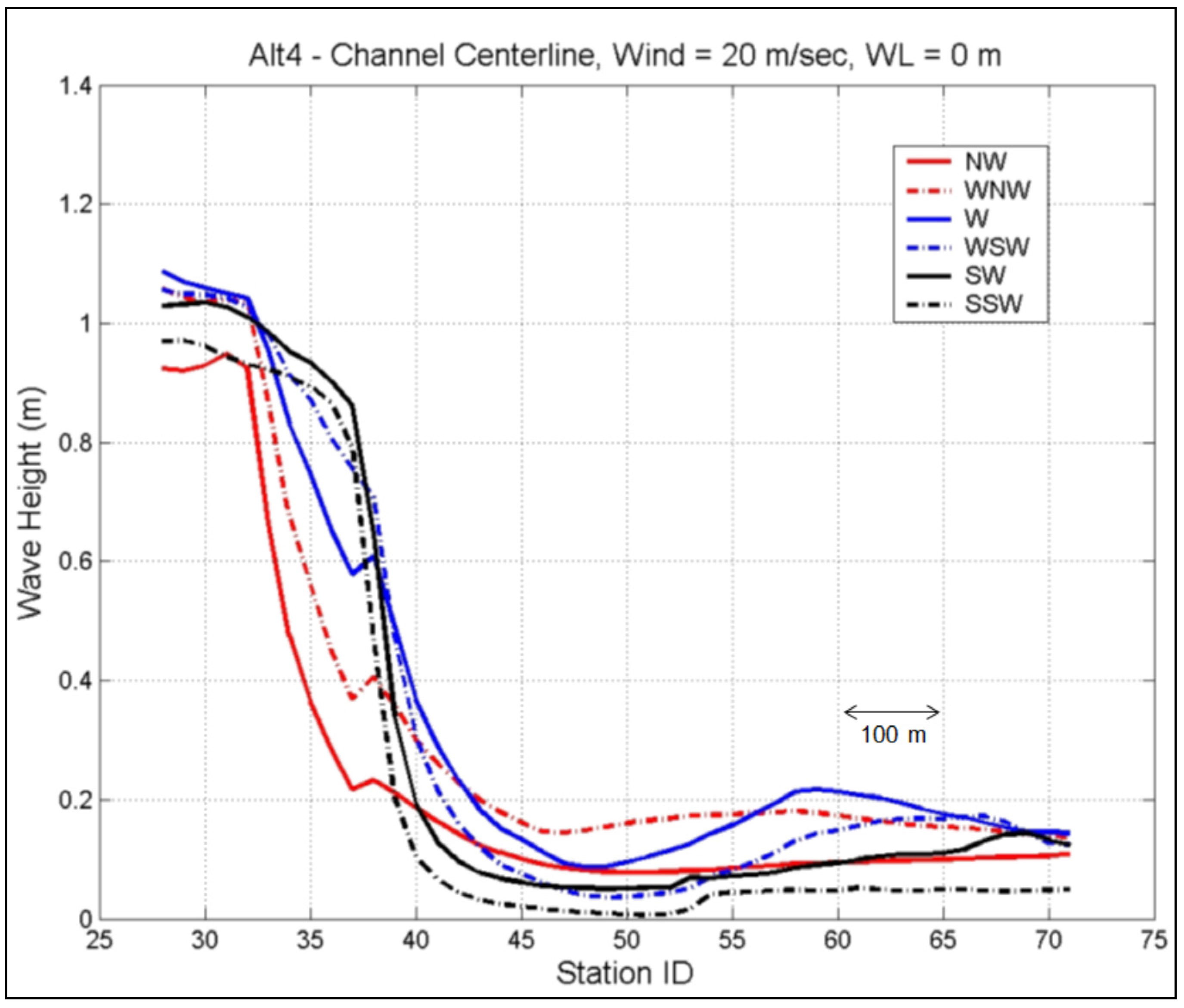
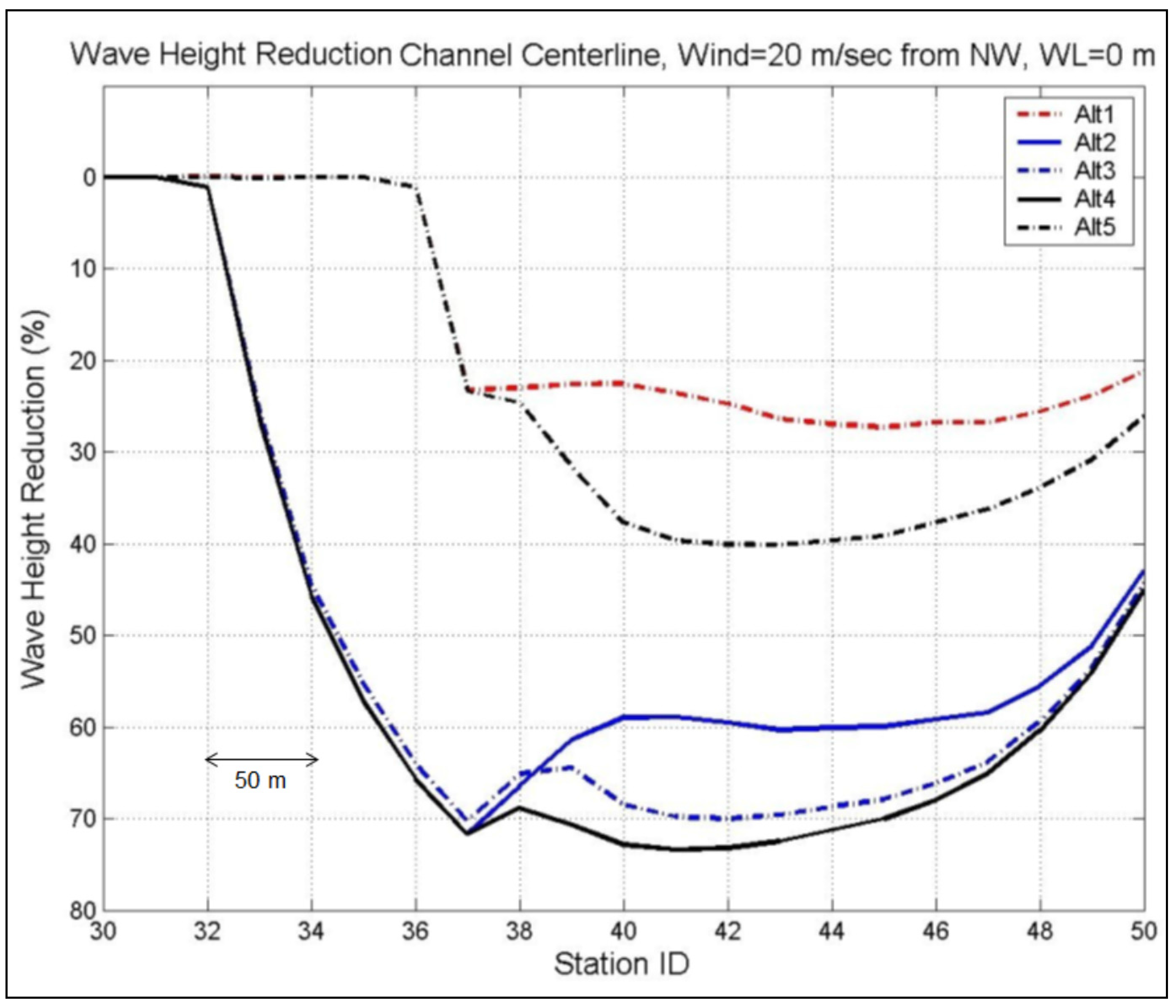
Figure 25 is an example of the calculated wave heights for Alt 4 along the west channel for all directions at 0 m water level. In these figures, incident waves are seen to decrease at Sta 32 (the western channel entrance). The long north jetty in Alts 2–4 has the location between Sta 32 and 38, whereas the short north jetty in Alts 1 and 5 has the location between Sta 36 and 38.
For all wind directions and both water levels investigated in this study, the analysis of wave height reduction from five alternatives is based on the wave height reduction factor calculated as the percentage of wave height reduction to the wave heights in the existing channel without the project condition:
Figure 19.
Model wave heights in the west channel for 50-year design wind from NW and WL = 0 m.
Figure 19.
Model wave heights in the west channel for 50-year design wind from NW and WL = 0 m.
Figure 20.
Model wave heights in the west channel for 50-year design wind from NW and WL = 1.5 m.
Figure 20.
Model wave heights in the west channel for 50-year design wind from NW and WL = 1.5 m.
Figure 21.
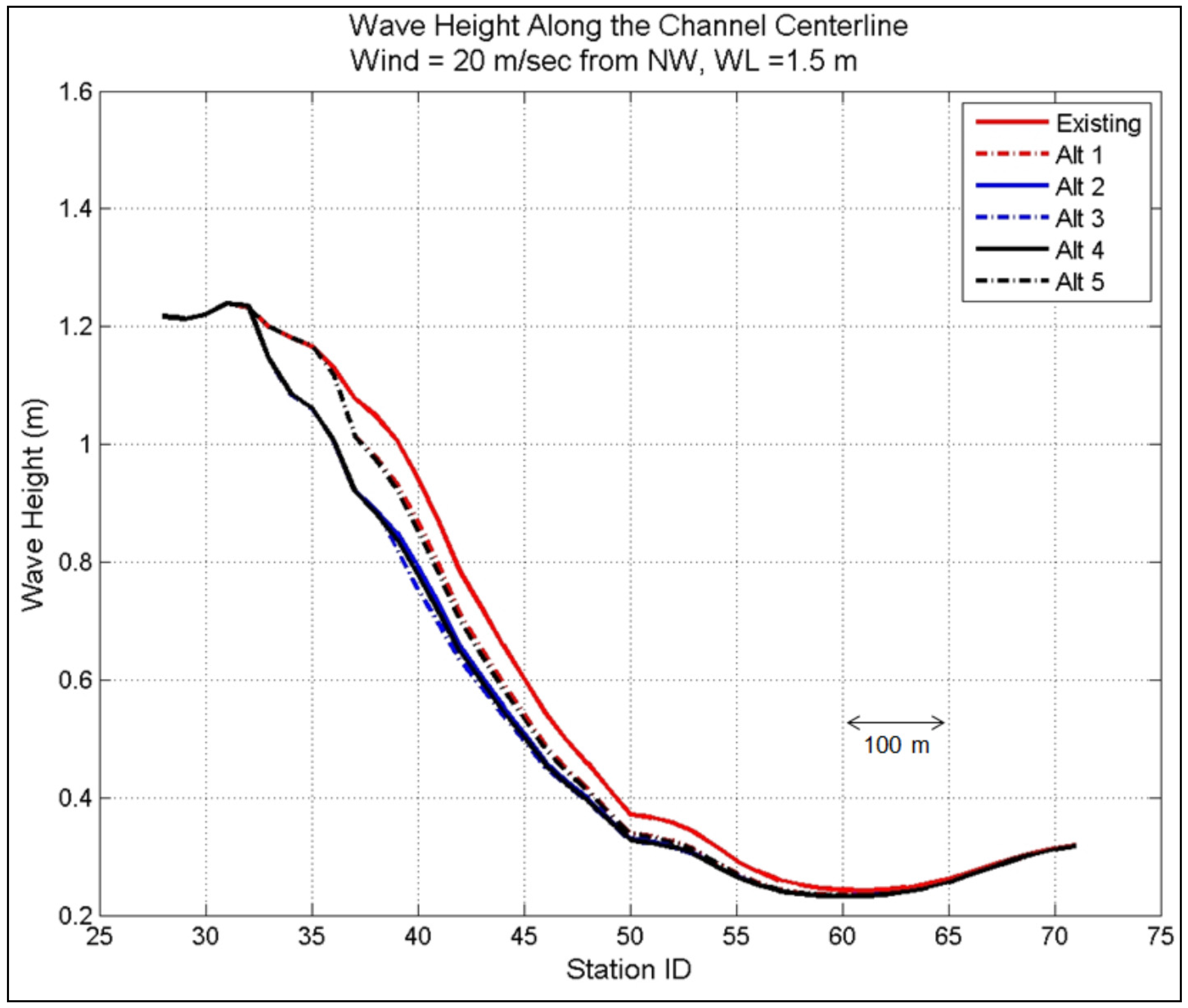
Model wave heights in the west channel for 50-year design wind from W and WL = 0 m.
Figure 21.
Model wave heights in the west channel for 50-year design wind from W and WL = 0 m.
Figure 22.
Model wave heights in the west channel for 50-year design wind from W and WL = 1.5 m.
Figure 22.
Model wave heights in the west channel for 50-year design wind from W and WL = 1.5 m.
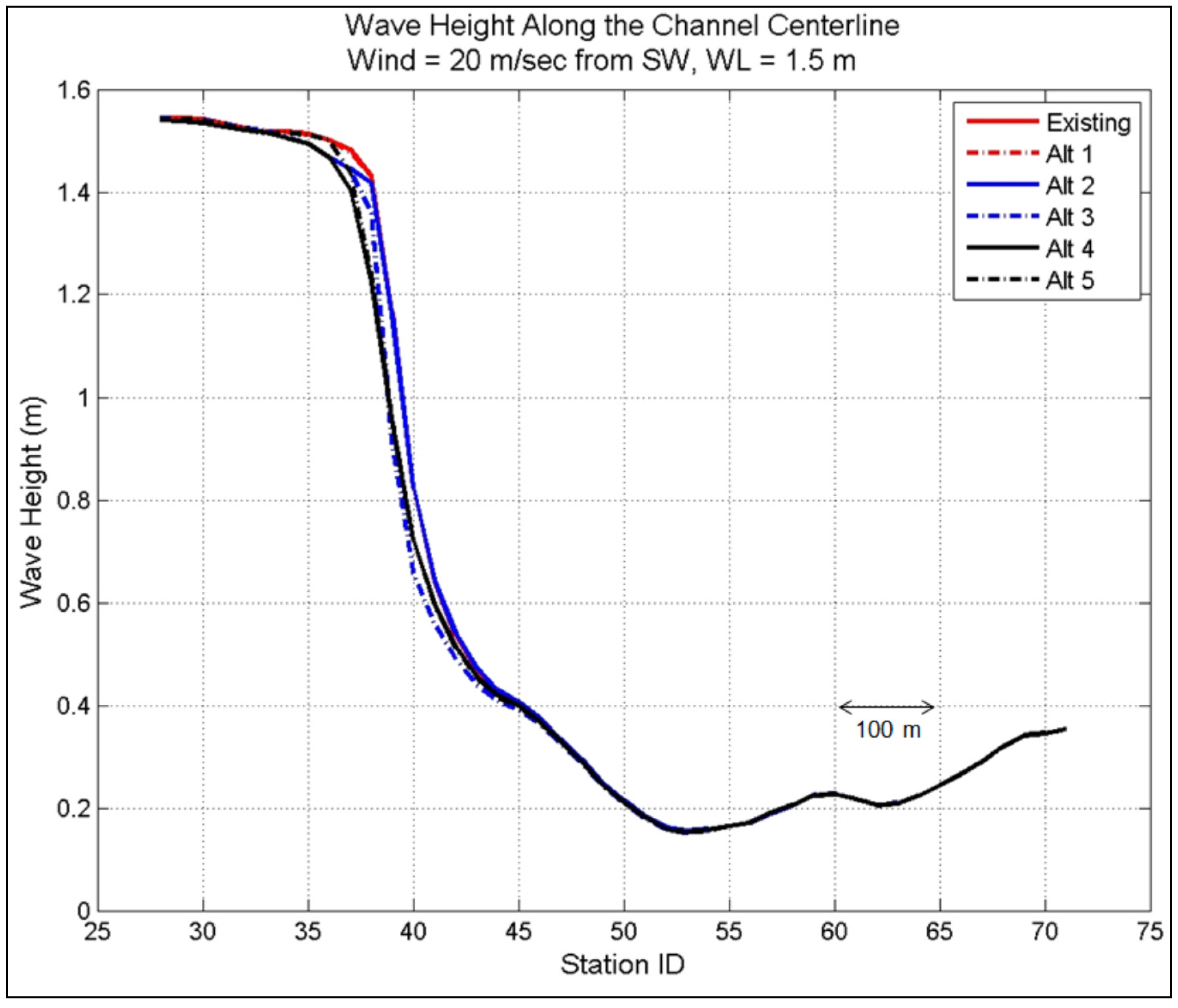
Figure 23.
Model wave heights in the west channel for 50-year design wind from SW and WL = 0 m.
Figure 23.
Model wave heights in the west channel for 50-year design wind from SW and WL = 0 m.
Figure 24.
Model wave heights in the west channel for 50-year design wind from SW and WL = 1.5 m.
Figure 24.
Model wave heights in the west channel for 50-year design wind from SW and WL = 1.5 m.
Figure 25.
Model wave heights for Alt 4 along the west channel for 50-year design wind from six directions (NW, WNW, W, WSW, SW, and SSW) and WL = 0 m.
Figure 25.
Model wave heights for Alt 4 along the west channel for 50-year design wind from six directions (NW, WNW, W, WSW, SW, and SSW) and WL = 0 m.
For example,
Figure 26,
Figure 27 and
Figure 28 show the wave height reduction factor along the channel centerline for Alternatives 1 to 5 for 50-year design winds from directions of NW,W,SW, respectively, and WL = 0 m.
Figure 26.
Calculated wave height reduction for Alts 1–5 along the west channel centerline for 50-year design wind from NW and WL = 0 m.
Figure 26.
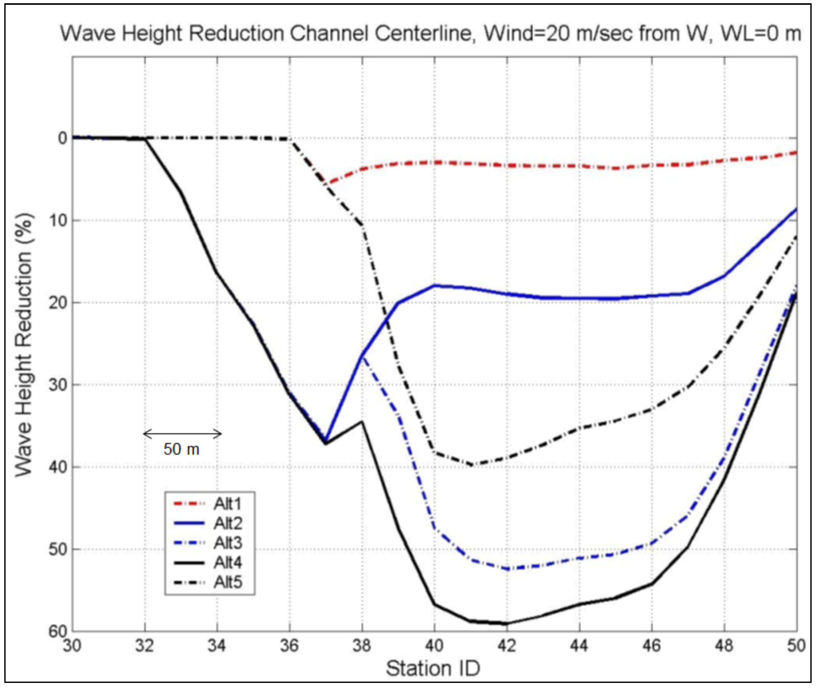
Calculated wave height reduction for Alts 1–5 along the west channel centerline for 50-year design wind from NW and WL = 0 m.
Figure 27.
Calculated wave height reduction for Alts 1–5 along the west channel centerline for 50-year design wind from W and WL = 0 m.
Figure 27.
Calculated wave height reduction for Alts 1–5 along the west channel centerline for 50-year design wind from W and WL = 0 m.
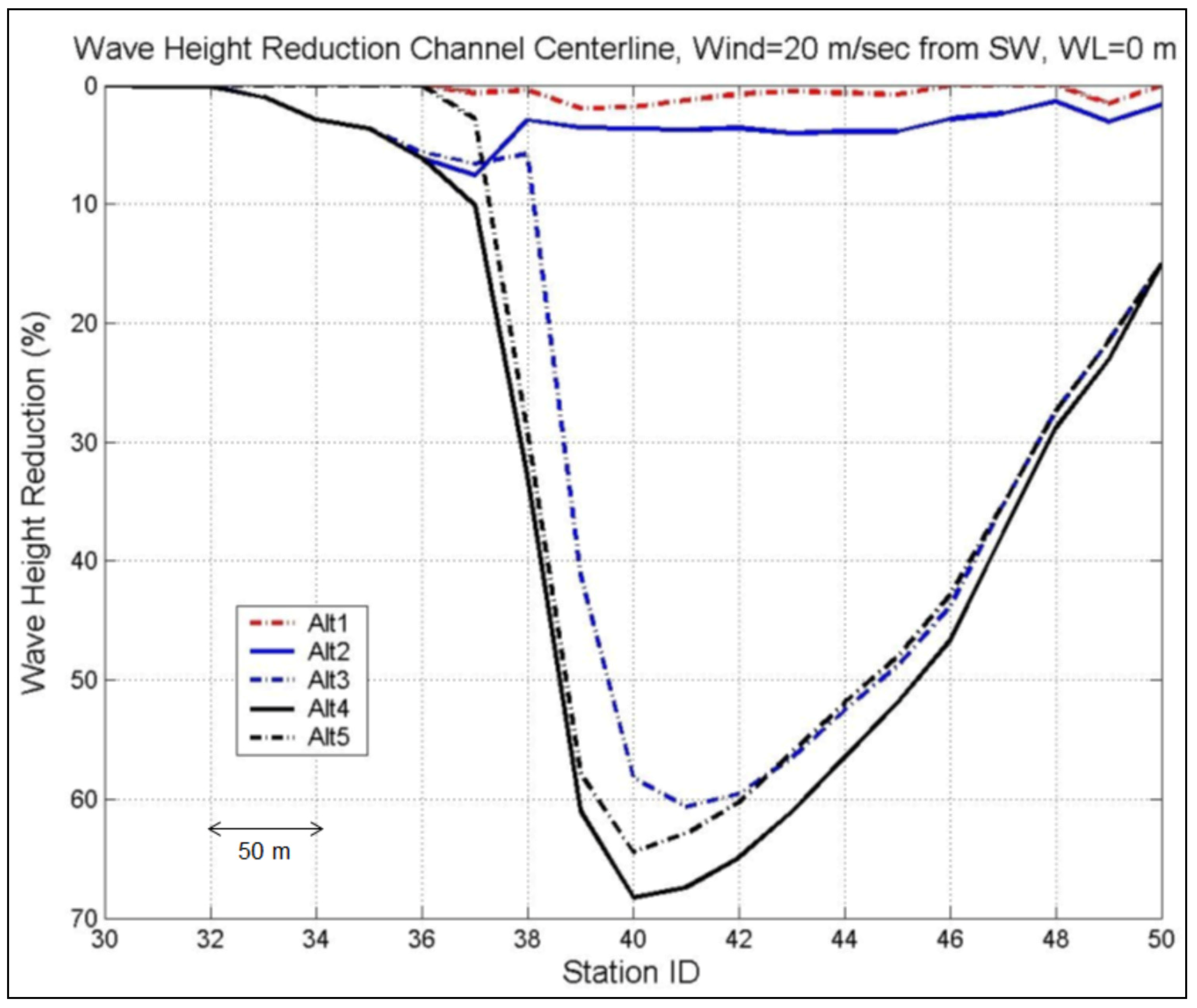
Figure 28.
Calculated wave height reduction for Alts 1–5 along the west channel centerline for 50-year design wind from SW and WL = 0 m.
Figure 28.
Calculated wave height reduction for Alts 1–5 along the west channel centerline for 50-year design wind from SW and WL = 0 m.
Among all the alternatives, Alts 3 and 4 produced the largest wave reduction for WL = 0 m and 1.5 m, respectively, along the west channel centerline and north and south shorelines. Larger waves are obtained for WL = 1.5 m as compared to WL = 0 m. It is noted that for WL = 1.5 m, the structures used in the alternatives will be submerged, losing much of their effectiveness to intercept and reduce wave energy propagating into the west and mid-sections of the channel. Under such extreme water level conditions, the wave height reduction cannot be used as a measure to rank the alternatives. Consequently, the ranking of alternatives is based on their performance (e.g., wave height reduction factor) calculated for WL = 0 m.
5.2. Hurricane Isabel
A similar analysis of waves was performed using Hurricane Isabel for the existing channel and five alternatives. The analysis was to estimate waves and water levels for a 50-year hurricane event. Because Hurricane Isabel approached the Chesapeake Bay from the southeast, the strong easterly winds associated with the hurricane produced elevated water levels along the west side of the bay and lowered the water level along the east side of bay. As a consequence, relatively lower waves had occurred at and around Tangier Island during Isabel. The wind and water level pattern associated with Hurricane Isabel was simulated for 17–23 September 2003. Both surface wind and pressure fields, used as input in the CMS, were generated from a PBL numerical model for tropical storms [
21].
Figure 29 shows an example of the calculated maximum wave field in the Bay (regional grid), and at Tangier Island (local grid) for the existing channel configuration during Isabel. Model results indicated comparatively lower waves and water levels at Tangier Island than in the western portion of the bay.
Figure 30 compares calculated high water levels (~1.5 m MTL) to data at NOAA Stations 8635750 (Lewisetta, VA) and 8636580 (Windmill Point, VA) during Isabel.
Figure 29.
Calculated maximum wave height fields during Hurricane Isabel.
Figure 29.
Calculated maximum wave height fields during Hurricane Isabel.
Figure 30.
Calculated and measured water levels at NOAA Stations 8635750 (Lewisetta, VA) and 8636580 (Windmill Point, VA) under Hurricane Isabel.
Figure 30.
Calculated and measured water levels at NOAA Stations 8635750 (Lewisetta, VA) and 8636580 (Windmill Point, VA) under Hurricane Isabel.
5.3. Estimates for Structure Design
Table 3 presents the average of wave height reduction factors at WL = 0 m along the west channel centerline at Sta 30 to 50 (
Figure 18) for five alternatives.
Table 4 and
Table 5 present the average wave height reduction factors at WL = 0 m along the north shoreline (Sta 5 to 25) and along the south shoreline (Sta 74 to 80), respectively. The average of wave height reduction factor is provided for nine wind directions with the average of cases of all nine wind directions for each alternative. Results indicate the wave reduction for Alt 4 was greater than other alternatives for WL = 0 m.
Table 3.
Average wave height reduction factors along channel centerline (Sta 30 to 50) at WL = 0 m.
Table 3.
Average wave height reduction factors along channel centerline (Sta 30 to 50) at WL = 0 m.
| Wind Dir | Alt 1 | Alt 2 | Alt 3 | Alt 4 | Alt 5 |
|---|
| N | 20.3 | 53.9 | 57.4 | 56.5 | 27.3 |
| NNW | 21.5 | 51.9 | 55.0 | 56.7 | 28.6 |
| NW | 16.4 | 48.6 | 52.0 | 54.0 | 22.9 |
| WNW | 5.6 | 31.2 | 38.5 | 40.7 | 14.4 |
| W | 2.2 | 16.7 | 31.4 | 35.1 | 18.5 |
| WSW | 1.1 | 7.7 | 30.9 | 36.1 | 27.1 |
| SW | 0.5 | 2.9 | 26.0 | 30.4 | 27.4 |
| SSW | 0.1 | 2.8 | 38.2 | 43.9 | 38.4 |
| S | 0.2 | 2.1 | 25.7 | 30.6 | 28.1 |
| Average | 7.5 | 24.2 | 39.5 | 42.7 | 25.9 |
Table 4.
Average of wave height reduction factors along north shoreline (Sta 5 to 25) at WL = 0 m.
Table 4.
Average of wave height reduction factors along north shoreline (Sta 5 to 25) at WL = 0 m.
| Wind Dir | Alt 1 | Alt 2 | Alt 3 | Alt 4 | Alt 5 |
|---|
| N | 38.4 | 57.5 | 61.6 | 61.2 | 44.9 |
| NNW | 39.6 | 55.9 | 59.0 | 60.5 | 46.2 |
| NW | 34.2 | 51.3 | 54.6 | 56.9 | 40.4 |
| WNW | 23.0 | 40.3 | 47.2 | 50.4 | 31.4 |
| W | 15.3 | 24.8 | 37.8 | 42.3 | 29.3 |
| WSW | 12.3 | 17.3 | 35.6 | 40.6 | 34.4 |
| SW | 11.2 | 15.5 | 37.2 | 40.6 | 36.9 |
| SSW | 10.8 | 15.7 | 40.5 | 46.9 | 40.8 |
| S | 11.4 | 20.0 | 45.6 | 50.9 | 42.1 |
| Average | 21.8 | 33.1 | 46.6 | 50.0 | 38.5 |
Table 5.
Average of wave height reduction factors along south shoreline (Sta 74 to 80) at WL = 0 m.
Table 5.
Average of wave height reduction factors along south shoreline (Sta 74 to 80) at WL = 0 m.
| Wind Dir | Alt 1 | Alt 2 | Alt 3 | Alt 4 | Alt 5 |
|---|
| N | 18.3 | 56.3 | 74.0 | 63.6 | 35.8 |
| NNW | 16.6 | 48.4 | 65.7 | 65.6 | 35.3 |
| NW | 8.7 | 34.9 | 52.2 | 53.2 | 24.9 |
| WNW | 2.4 | 17.4 | 36.7 | 40.3 | 17.3 |
| W | 1.6 | 11.0 | 37.7 | 42.7 | 25.4 |
| WSW | 0.7 | 4.4 | 41.6 | 45.9 | 36.5 |
| SW | 0.3 | 2.1 | 45.7 | 47.1 | 43.6 |
| SSW | 0 | 2.1 | 65.1 | 68.6 | 61.1 |
| S | 0 | 1.2 | 59.6 | 63.6 | 59.5 |
| Average | 5.4 | 20.0 | 53.1 | 54.5 | 37.7 |
With a higher water level scenario (WL = 1.5 m), the average wave reduction was less for all alternatives, about 25 percent less than the Existing Channel configuration (without project). Based on model results for 50-year wind forcing and Hurricane Isabel simulation, Alt 4 was more effective alternative overall in reducing wave energy propagation in the canal than the other alternatives at WL = 0 m. It is noted that at the higher water level WL = 1.5 m, the structures evaluated would be either partially or fully submerged, thereby diminishing their effectiveness to intercept and reduce wave energy penetrating into the west and mid-sections of the channel. At this higher water level, wave height reduction cannot be used as a proper measure to evaluate the alternatives.
The bottom lines in
Table 3,
Table 4 and
Table 5 give the wave reduction factors for each alternative averaged over nine wind directions along the channel centerline, north shoreline, and south shoreline, respectively. By averaging results for the centerline and north and south shoreline, the overall representative wave reduction rating was calculated in
Table 6. Among all alternatives, Alt 4 yielded the highest representative wave reduction.
Table 6.
Representative wave reduction ratings for Alts 1 to 5.
Table 6.
Representative wave reduction ratings for Alts 1 to 5.
| Alternative | Alt 1 | Alt 2 | Alt 3 | Alt 4 | Alt 5 |
|---|
| Average Wave Reduction (%) | 11.6 | 25.8 | 46.4 | 49.1 | 34.0 |
5.4. Channel Sedimentation
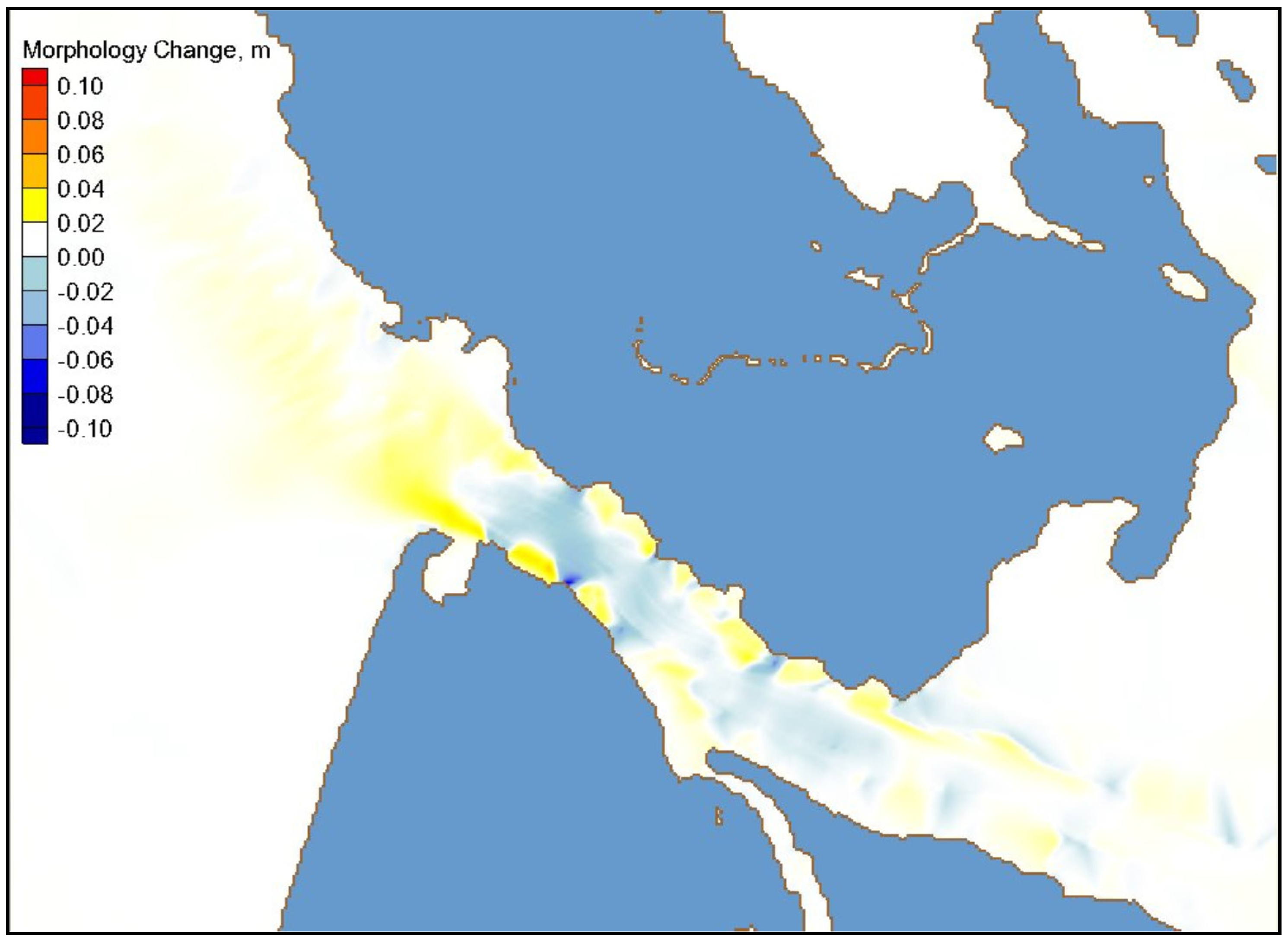
The proposed alternatives may affect the overall sedimentation pattern in the vicinity of the structures and throughout the channel reaches of Tangier Island. To address this concern, the CMS was used to simulate the sediment transport for Hurricane Isabel. The purpose of the sediment simulation was to provide a quick view of potential shoaling and erosion areas for a 50-year tropical storm condition. It was by no means to model the long-term morphology evolution at Tangier Island. In the absence of sediment grain sized distribution data, a constant sediment median size of 0.15 mm was assumed in this simulation.
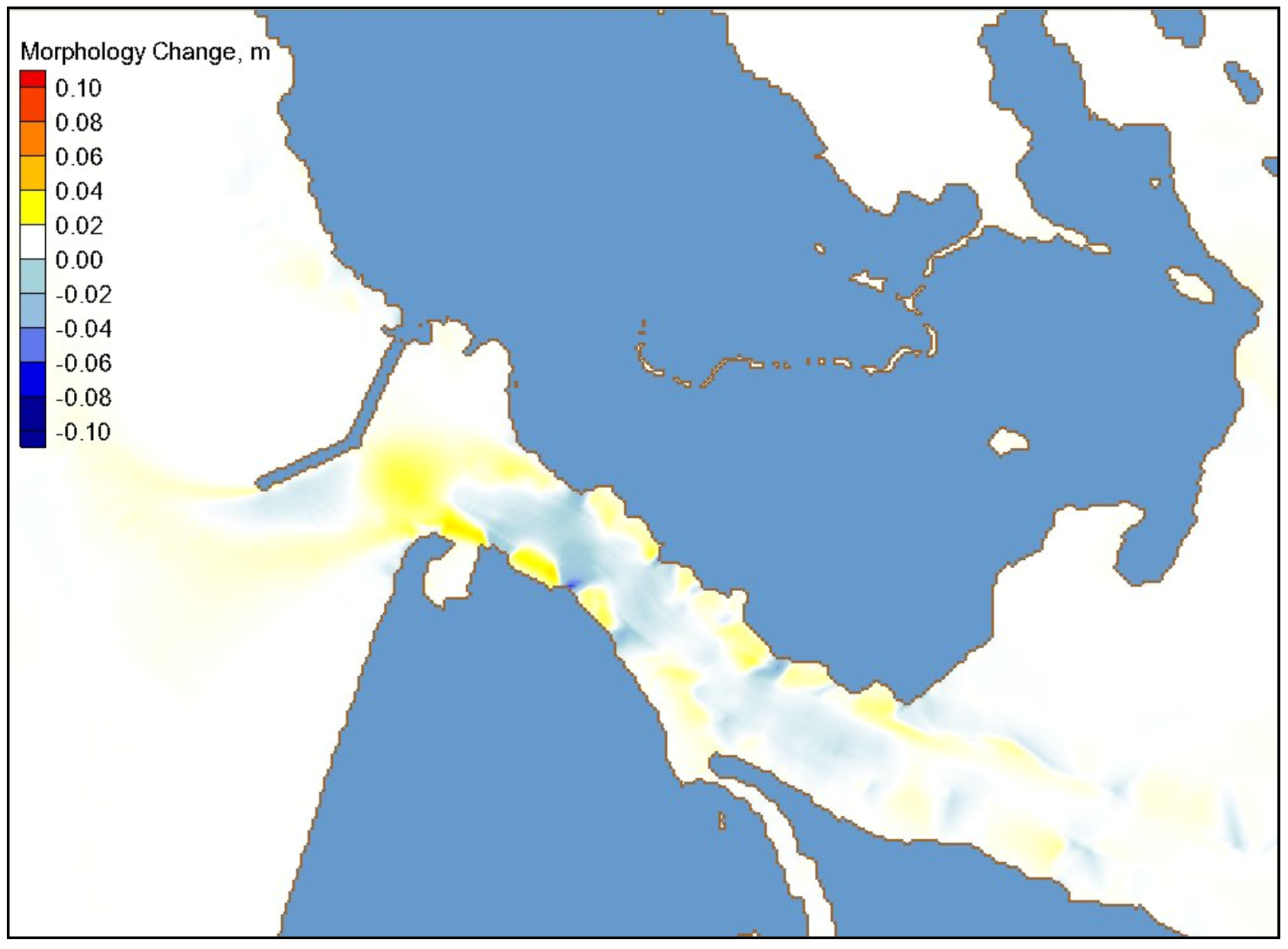
Figure 31 shows the calculated spatially varying sediment accretion and erosion field for the existing west channel configuration (without project) in the simulation of Hurricane Isabel. Model results show sediment deposition immediately outside the west entrance channel and bottom erosion inside the west entrance channel.
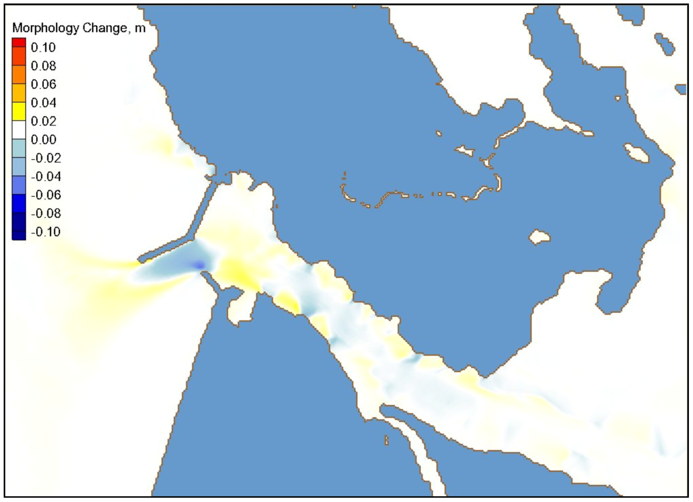
Figure 32 and
Figure 33 show calculated erosion and deposition fields in the simulation of Isabel for Alts 2 and 4, respectively. Model results showed sediment scouring in the channel near the tip of the breakwater and getting trapped inside the west entrance channel. More bottom erosion occurred between the north breakwater and south spur structure in Alts 4 and 5. The eroded sediment was carried by the stronger current into the bay, and the sediment deposition was insignificant inside the west channel entrance.
Figure 31.
Model sediment accretion and erosion for the existing configuration under Hurricane Isabel.
Figure 31.
Model sediment accretion and erosion for the existing configuration under Hurricane Isabel.
Figure 32.
Calculated sediment accretion and erosion for Alt 2 under Hurricane Isabel.
Figure 32.
Calculated sediment accretion and erosion for Alt 2 under Hurricane Isabel.
Figure 33.
Calculated sediment accretion and erosion field for Alt 4 under Hurricane Isabel.
Figure 33.
Calculated sediment accretion and erosion field for Alt 4 under Hurricane Isabel.
Overall, sediment transport results for the existing channel configuration and all five alternatives were similar, showing an insignificant morphology change (magnitude of either erosion or deposition less than 2 in. or 0.05 m). While the structures are intended to reduce wave energy in the channel, the currents increase and scour channel near the structures. Some additional settling of suspended sediments occurred away from the channel due to reduced wave-induced currents. Based on the model results for the 50-year return interval tropical storm (Hurricane Isabel), the depth-averaged current magnitude was less than 3 ft/s (1 m/s) in the channel and the maximum channel depth change was less than 2 in. (0.05 m). Therefore, the combined tidally-driven and wave-driven currents in the channel are usually below the threshold for the initiation of sediment motion. No significant effect of structure on channel sedimentation and channel infilling was apparent in the Hurricane Isabel simulation.
6. Summary and Conclusions
Numerical modeling of waves and currents was conducted to assess the impacts of these environmental forces on jetty alternatives to protect a shallow draft navigation channel entrance on Tangier Island, VA, located in the south Chesapeake Bay. The Coastal Modeling System (CMS), an integrated numerical tool that includes a spectral wave model, a two-dimensional depth-averaged hydrodynamic model with sediment transport calculations, is used to investigate the potential effects of waves and hydrodynamics on a relocation and replacement dock.
The existing channel geometry and five alternatives were investigated using the CMS, an integrated wave-hydro-sediment transport modeling system. The five alternatives evaluated consisted of a breakwater system that included a low crest jetty connecting to the north shoreline. Alts 3, 4, and 5 had an optional short structure (spur) joining to the south shoreline. Structural design estimates are based on findings of numerical wave and hydrodynamic modeling conducted for the 50-year design wind speeds, waves, and two water levels. The 50-year wind speed was considered as idealized condition and was based on a previous study by Basco and Shin [
22]. Different structure alternatives were evaluated to determine an optimal design, as determined by the level of wave energy reduction in the navigation channel. The hydrodynamic modeling study results (e.g., wave height, period, direction, and water level) along the western side of the proposed structure footprint were used in these preliminary wave control structural design calculations. These calculations include structural stability, run-up/overtopping, and transmission through and over the structure.
Overall, Alt 4 performed better than the other alternatives in its protection of the boat canal entrance. However, some of the other alternatives also provided considerable wave reduction benefits. The comparison of the alternatives shows that Alts 3, 4, and 5 with south spur jetty outperformed Alts 1 and 2 with no south spur for reducing the wave energy in the channel.
It should be noted that the geometry of the channel itself, even without any jetty structure, helps to dampen the propagating waves in the boat canal. For example, at Sta 50, located approximately 300 m (1000 ft) down the channel from the western entrance, the wave energy has dissipated to the extent that wave height is reduced to 10% to 20% of the height in the bay. Thus, while the CMS shows that Alt 4 provides the greatest wave reduction benefits amongst the five alternatives, multiple criteria may be used in the selection of the optimal alternative for the final design. In closing, this modeling study provides estimates of waves and currents necessary for a follow-up structural design study that will determine the final length, orientation, elevation, and width of the structure system and foundation requirements.
Acknowledgments
The authors would like to thank both of the USACE district, Norfolk, and ERDC Navigation RD & T program for supporting and funding the study. Special thanks go to Julie D. Rosati for her continual support and encouragement towards development and improvement of the CMS. Permission was granted by the Chief, USACE to publish this information.
Author Contributions
All authors have conceived, formulated, conducted, and contributed to the work described in this paper. L.L and Z.D. wrote the first version of the manuscript and D.W. and D.K. edited the paper. All authors read and approved the final manuscript.
Conflicts of Interest
The authors declare no conflict of interest.
References
- Boon, J.D.; Brubaker, J.M.; Forrest, D.R. Chesapeake Bay Land Subsidence and Sea Level Change—An Evaluation of Past and Present Trends and Future Outlook; Virginia Institute of Marine Science Special Report, No. 425; VIMS, Gloucester Point: Norfolk, VA, USA, 2010. [Google Scholar]
- Demirbilek, Z.J.; Rosati, J. Verification and Validation of the Coastal Modeling System, Report 1: Summary Report; ERDC/CHL Technical Report 11-10; U.S. Army Corps of Engineers Research and Development Center: Vicksburg, MS, USA, 2011. [Google Scholar]
- Zundel, A.K. Surface-Water Modeling System Reference Manual—Version 9.2; Brigham Young University Environmental Modeling Research Laboratory: Provo, UT, USA, 2006. [Google Scholar]
- Lin, L.; Rosati, J.; Demirbilek, Z. CMS-Wave Model: Part 5. Full-Plane Wave Transformation and Grid Nesting; ERDC/CHL CHETN-IV-81; U.S. Army Corps of Engineers Research and Development Center: Vicksburg, MS, USA, 2012. [Google Scholar]
- Coastal Modeling System. Available online: http://cirpwiki.info/wiki/CMS (accessed on 8 September 2015).
- Demirbilek, Z.; Lin, L.; Hayter, E.; O’Connell, C.; Mohr, M.; Chader, S.; Forgette, C. Modeling of Waves, Hydrodynamics and Sediment Transport for Protection of Wetlands at Braddock Bay, NY; ERDC TR-14-8; U.S. Army Corps of Engineers Research and Development Center: Vicksburg, MS, USA, 2015. [Google Scholar]
- Lambert, S.S.; Willey, S.S.; Campbell, T.; Thomas, R.C.; Li, H.; Lin, L.; Welp, T.L. Regional Sediment Management Studies of Matagorda Ship Channel and Matagorda Bay System, Texas; ERDC/CHL TR-13-10; U.S. Army Corps of Engineers Research and Development Center: Vicksburg, MS, USA, 2013. [Google Scholar]
- Lin, L.; Reed, C.W. Numerical modeling of mixed sediment transport in GIWW and West Galveston Bay, Texas. In Proceedings of the 8th International Symposium on Coastal Engineering and Science of Coastal Sediment Processes, Coastal Sediments’15, San Diego, CA, USA, 11–15 May 2015.
- Lin, R.Q.; Lin, L. Wind input function. In Proceedings of the 8th International Workshop on Wave Hindcasting and Prediction, Oahu, HI, USA, 14–19 November 2004.
- Lin, L.; Lin, R.Q. Wave breaking function. In Proceedings of the 8th International Workshop on Wave Hindcasting and Prediction, Oahu, HI, USA, 14–19 November 2004.
- Lin, R.Q.; Lin, L. Wave breaking energy in coastal region. In Proceedings of the 9th International Workshop on Wave Hindcasting and Prediction, Victoria, BC, Canada, 24–29 September 2006.
- Li, H.; Lin, L.; Burks-Copes, K. Numerical modeling of coastal inundation and sedimentation by storm surge, tides, and waves at Norfolk, Virginia, USA. In Proceedings of the 33rd International Conference on Coastal Engineering, Santander, Spain, 1–6 July 2012.
- Demirbilek, Z.; Lin, L.; Ward, D.L.; King, D.B. Modeling Study for Tangier Island Jetties, Tangier Island, VA; ERDC/CHL TR-14-8; U.S. Army Corps of Engineers Research and Development Center: Vicksburg, MS, USA, 2015. [Google Scholar]
- Lopez-Feliciano, O.L.; Herrington, T.O.; Miller, J.K. A Morphology change study using the CMS in a groin field during Hurricane Sandy. J. Am. Shore Beach 2015, 83, 19–26. [Google Scholar]
- Lin, L.; Demirbilek, Z.; Mase, H.; Zheng, J.; Yamada, F. A Nearshore Spectral Wave Processes Model for Coastal Inlets and Navigation Projects; ERDC/CHL TR-08-13; U.S. Army Corps of Engineers Research and Development Center: Vicksburg, MS, USA, 2008. [Google Scholar]
- Lin, L.; Demirbilek, Z. Recent capabilities of CMS-Wave: A coastal wave model for inlets and navigation projects. J. Coast. Res. 2011. [Google Scholar] [CrossRef]
- Lin, L.; Lin, R.Q.; Maa, J.P.Y. Numerical simulation of wind wave field. In Proceedings of the 9th International Workshop on Wave Hindcasting and Forecasting, Victoria, BC, Canada, 24–29 September 2006.
- Vimswave-Vims Directional Wave Data. Available online: http://web.vims.edu/physical/research/VIMSWAVE/VIMSWAVE.htm (accessed on 8 September 2015).
- Turning Operational Oceanographic Data into Meaningful Information for the Nation. Available online: https://tidesandcurrents.noaa.gov (accessed on 8 September 2015).
- Demirbilek, Z.; Lin, L.; Bass, G.P. Prediction of storm-induced high water levels in Chesapeake Bay. In Proceedings of the Coastal Disaster 2005 Conference, ASCE, Charleston, SC, USA, 8–11 May 2005.
- Demirbilek, Z.; Lin, L.; Mark, D.J. Numerical modeling of storm surges in Chesapeake Bay. Int. J. Ecol. Dev. 2008, 10, 24–39. [Google Scholar]
- Basco, D.R.; Shin, C.S. Design Wave Information for Chesapeake Bay and Major Tributaries in Virginia; Technical Report, No. 93-1; Department of Civil Engineering, The Coastal Engineering Institute, Old Dominion University: Norfolk, VA, USA, 1993. [Google Scholar]
© 2015 by the authors; licensee MDPI, Basel, Switzerland. This article is an open access article distributed under the terms and conditions of the Creative Commons Attribution license ( http://creativecommons.org/licenses/by/4.0/).


