3.1. Hydrodynamic Model
The hydrodynamic conditions were simulated using Delft3D-FLOW [
49]. The model has been successfully applied within oceanic, coastal, estuarine, riverine, and flooding conditions [
49,
50,
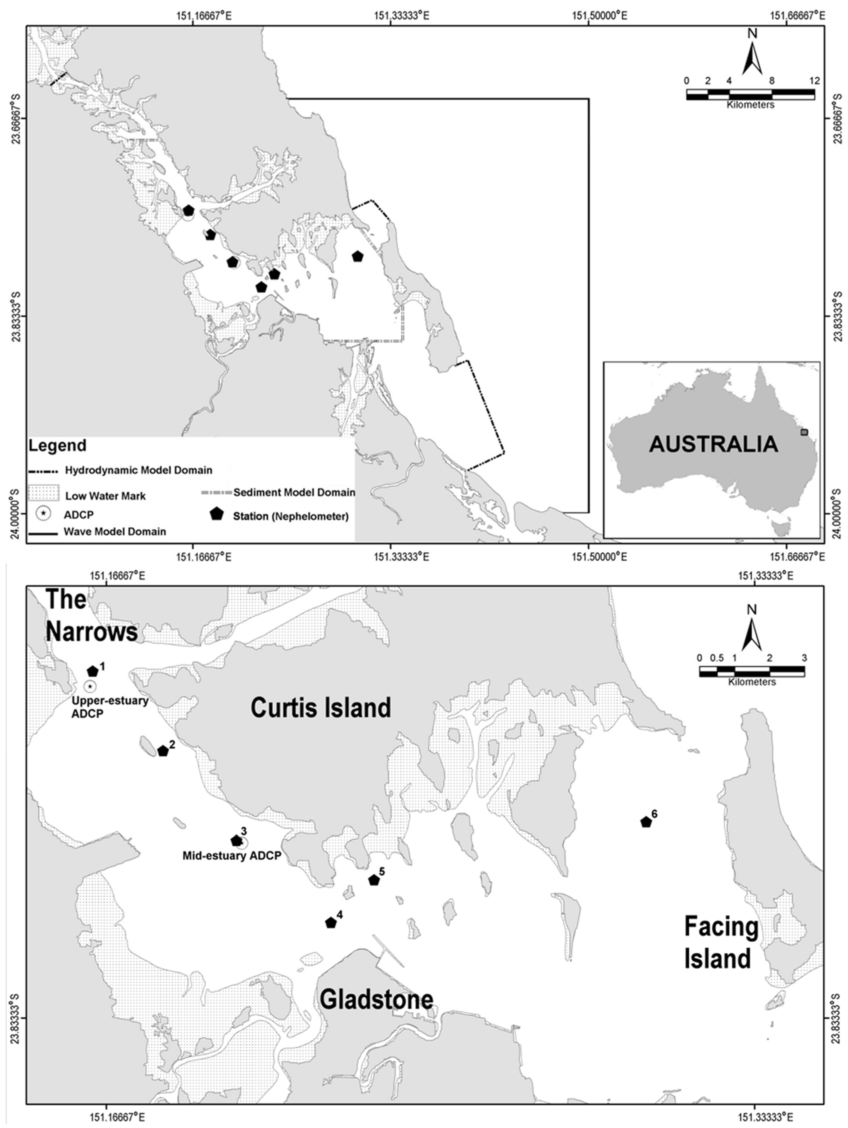
51]. A curvilinear computational grid with varying cell size was developed for the entire extent of the estuary. The finest grid resolution (25 m) was defined along shorelines and regions of steep depth gradients, to accurately define the current patterns. Whilst the coarsest resolution (~400 m) was applied in the outer region nearby the southern entrances of the estuary and neighbouring coastal waters (
Figure 1). Datasets used to represent the bathymetry of the estuary were sourced from commercial nautical charts and bathymetric surveys [
52]. In order to define the three-dimensional current structure, a σ-layer approach was employed with five equally-proportioned vertical layers throughout the model domain. Tidal variations were driven at the open boundaries of the model domain through the northern entrance using water elevation data from Port Alma tidal station (23.58° S, 150.87° E) and the eastern entrances using data from the Gatcombe Head tidal station (23.88° S, 151.37° E).
The “cyclic” advection schemes for momentum and transport were selected. The κ-ε turbulence closure scheme was selected for the vertical viscosity formulation, with background values set to 0 m
2/s. The Manning roughness formula was used to account for the bottom friction, with a uniform coefficient of 0.02 selected as representative of the seabed in the region on the basis of previous works by Wolanski
et al. [
53] and King and Wolanski [
54]. The horizontal eddy viscosity was set to 1 m
2/s throughout the model domain. Hourly wind speed and direction data, measured at the Gladstone Airport by the Australian Bureau of Meteorology (station identification: 039326; 23.87° S, 151.22° E), was used to account for the wind forcing across the model domain. The wind drag coefficients, C
D, is assumed to vary linearly with wind speed from 0.00063 to 0.00723 over the range of U
10 = 0–100 m/s. The model time-step was set to 0.2 min, which produced Courant numbers less than 10.
3.2. Wave Model
The SWAN model [
55] was used to reproduce the prevailing wave conditions. The model is fully spectral (in all directions and frequencies) and computes the evolution of wind waves in coastal regions with shallow water depths. The physical processes selected for the simulations were: white-capping, depth-induced wave-breaking, bottom friction, and triad wave-wave interactions. Using an unstructured triangular mesh approach, the generated computational grid included the entire Port Curtis estuary and offshore regions (24.00° S, 151.50 °E to 23.65° S, 151.50° E,
Figure 1). A fine (<50 m) mesh resolution was defined for tidal creeks and shorelines and a coarser mesh resolution (>500 m) was applied over the estuary region and near the open boundaries of the domain. The bathymetric dataset used for the wave model was sourced, as per the hydrodynamic modelling. Surface waves entering the model boundaries were obtained from the WAVEWATCH III
® (WW3) global model (National Centres for Environmental Prediction National Oceanic and Atmospheric Administration, College Park, MD, USA) [
56]. Outputs of WW3 (significant wave height (H
s), mean wave period (T
p) and peak wave direction period (P
dir)) were extracted from the computational point closest to the area of interest (24.00° S, 152.50° E) and used for the model simulations. Model surface and open boundary data were updated at hourly intervals. The default SWAN parameterisation of depth-induced wave-breaking was employed (0.73 [
57]). Bottom friction was activated using the drag law-based model of Collins [
58] and a bottom friction coefficient of 0.01 was applied. In addition, quadruplet wave-wave interaction was also included. Hourly wind speed and direction data, measured at the Gladstone Airport by the Australian Bureau of Meteorology, was used as model input.
3.3. Sediment Transport Model
Suspended sediment concentrations (SSC) were modelled using a tailored version of DREDGEMAP, an enhancement of SSFATE [
48], a three-dimensional sediment transport and fates model, jointly developed by Applied Science Associates Pty Ltd and the U.S. Army Corps of Engineers (USACE) Environmental Research and Development Center (ERDC). The model has been successfully applied in coastal and estuarine settings [
59,
60,
61]. The model represents the total mass of sediments suspended over time by a defined sub-sample of Lagrangian particles, allocating an equal proportion of the mass to each particle, where the transport, dispersion and settling of suspended sediment released to the water column is calculated using a random-walk procedure. Sediment particles are divided into five size classes. For the purpose of this study the following grain size classes were adopted: 5 μm, 75 μm, 200 μm, 450 μm and 1000 μm.
Settling of mixtures of particles is a complex process due to interaction of the different size classes, some of which tend to be cohesive, and thus clump together to form larger particles that have different fall rates than would be expected from their individual sizes. Enhanced settlement rates, due to flocculation and scavenging, are particularly important for clay and fine-silt sized particles and as such these processes are implemented in DREDGEMAP.
Minimum sinking rates are calculated using Stokes equations, based on the size and density of the particle. However, sinking rates of finer classes (representing clay and silt-sized particles) are increased based on the local concentration of the same and larger particles, to account for clumping and entrainment.
The settling velocity of each particle size class (
), is computed from:
where:
Culi and
Clli are the nominal upper and lower concentration limits, respectively, for enhanced settling of grain size
i,
ai is a grain-size class average maximum floc settling velocity,
C is the total concentration for all grain size classes [
61].
whereas, if
then
Selected values for Culi, Clli and ai adopted for this study ranged between 1000–8000 mg/L, 50–400 mg/L and 0.0008–0.1 m/s, respectively. The settling velocity for the largest size class (1000 μm) was assumed constant at 0.1 m/s.
Deposition is calculated as a probability function of the prevailing bottom stress, local sediment concentration and size class. Mixing of re-suspended sediment into the water column is a dynamic balance between estimates of the sinking rate and vertical mixing induced by turbulence (as specified by vertical mixing coefficients).
Sediment deposition flux is computed as:
If
, then
Otherwise,
where:
Pi is the deposition probability of
i-th size class,
Ci is the sediment concentration,
Wsi is the calculated settling velocity and
bi is the empirical parameter that includes all other factors influencing deposition other than shear (0.2–1.0 for clays to fine sand) [
61].
Deposition probability, Pi, is calculated as follows:
P1, for clay sized particles (1st size class)
where: τ
cd is the critical shear stress for deposition for the clay fraction, for this study a value of 0.016 was adopted. The bottom shear stress is based on the combined velocity due to current and wave action using the parametric approximation by Soulsby [
62].
Pi, for the other size classes (2nd, 3rd and 4th size classes)
where:
τuli is the shear stress above which no deposition occurs for grain size class
i, and
τlli is the shear stress below which deposition probability for grain class
i is 1.0.
For values between τlli and τuli, linear interpolation was used. Adopted τuli and τlli values for this study ranged between 0.030–0.900 and 0.016–0.200, respectively, excluding the 1000 μm size class.
The model can employ two different re-suspension algorithms. The first is based on the work of Sanford and Maa [
63] and, subsequently, Lin
et al. [
64], and applies to material deposited in the last tidal cycle, which accounts for the fact that newly deposited material will not have had time to consolidate and will be re-suspended with less effort (lower shear force) than consolidated bottom material. The second algorithm, which was used in this study, is the established Van Rijn method [
65] and applies to all other material that has been deposited prior to the start of the last tidal cycle. This method calculates a constantly varying critical threshold for re-suspension, based on the median local particle-size distribution for settled material. Re-suspension algorithms implemented in DREDGEMAP are presented in detail by Swanson
et al. [
61].
Knowledge of the initial bed sediment distribution was critical in predicting suspended sediment concentrations. Surface sediment grain size contribution maps were established based on data sourced from the analysis of >650 sediment cores collected throughout the estuary [
66]. The contribution of five sediment size classes (5 μm, 75 μm, 200 μm, 450 μm and 1000 μm) throughout the estuary was spatially assigned and interpolated using the inverse distance weighting method [
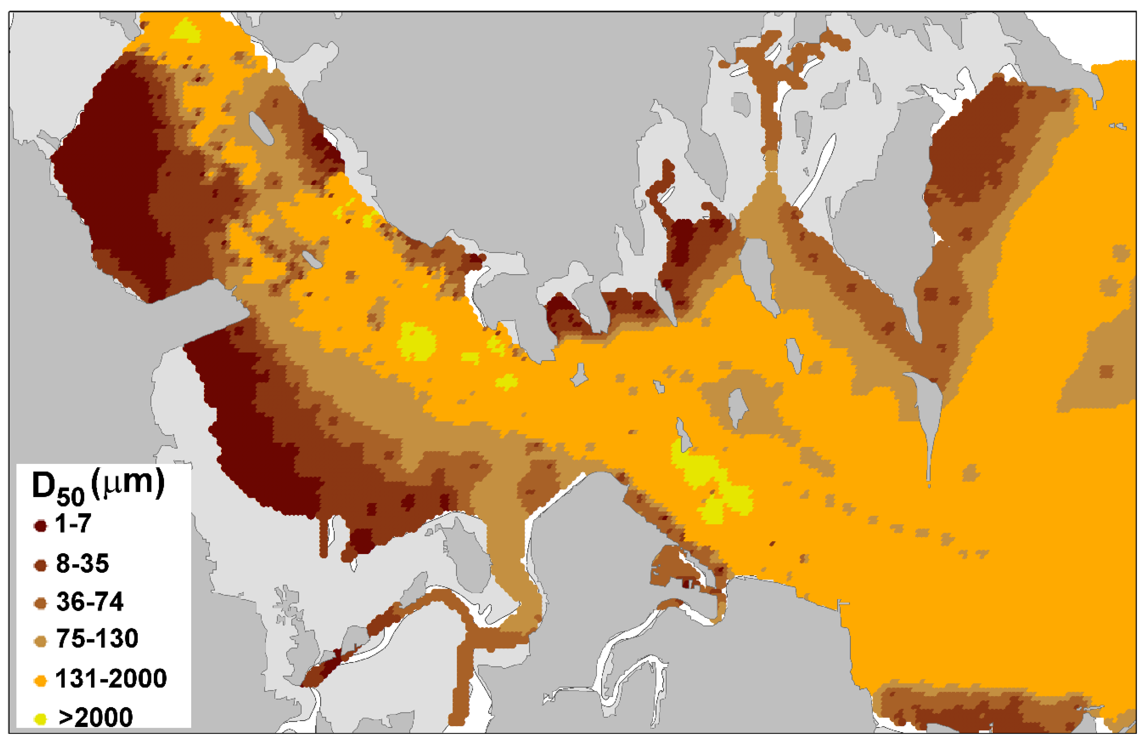
67] throughout the model domain. A grid resolution of 40 m was used throughout the model domain. Clays and silts dominate the shallow intertidal regions of the estuary, whilst larger sediments, including fine and coarse sands dominate the more energetic deeper channel regions of the estuary.
Figure 2 presents the median grain size (D
50) of the surface sediments of Port Curtis estuary used as part of the study. Measured sediment densities were incorporated into the model inputs. The sheltering effects of seagrass on shear stress [
68] and biologically-altered erodability of the bed sediments [
69,
70] was not included as part of the modelling approach.
Figure 2.
Surface sediment median grain size (D50) map of Port Curtis estuary (October 2010).
Figure 2.
Surface sediment median grain size (D50) map of Port Curtis estuary (October 2010).
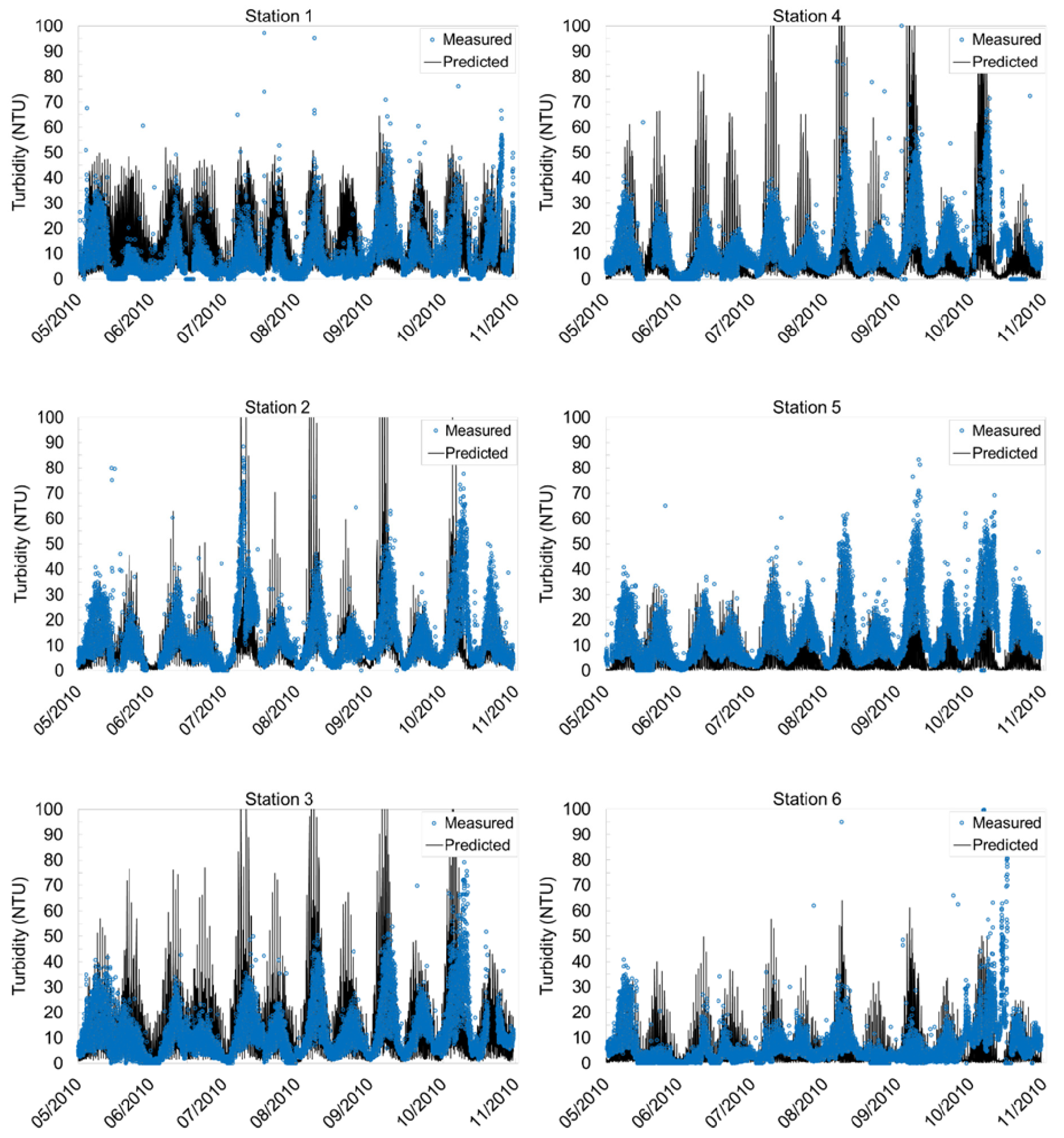
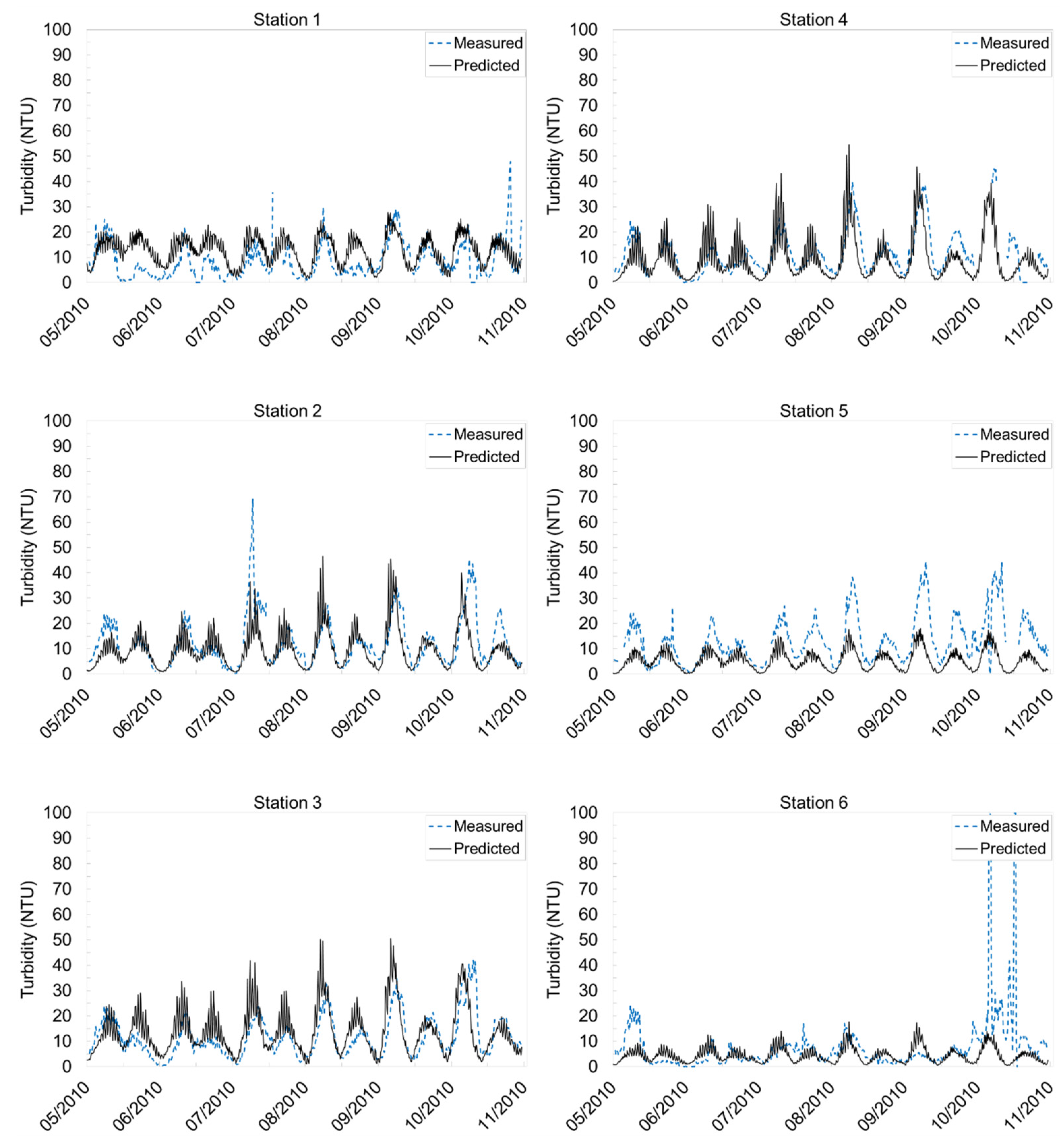
Model predictions output as SSC were converted to turbidity in order to provide comparison with coincident turbidity datasets collected at six stations. Suspended sediment concentrations were converted as follows [
71]:


