Formulating Fine to Medium Sand Erosion for Suspended Sediment Transport Models

Abstract

The capacity of an advection/diffusion model to predict sand transport under varying wave and current conditions is evaluated. The horizontal sand transport rate is computed by vertical integration of the suspended sediment flux. A correction procedure for the near-bed concentration is proposed so that model results are independent of the vertical resolution. The method can thus be implemented in regional models with operational applications. Simulating equilibrium sand transport rates, when erosion and deposition are balanced, requires a new empirical erosion law that involves the non-dimensional excess shear stress and a parameter that depends on the size of the sand grain. Comparison with several datasets and sediment transport formulae demonstrated the model’s capacity to simulate sand transport rates for a large range of current and wave conditions and sand diameters in the range 100–500 μm. Measured transport rates were predicted within a factor two in 67% of cases with current only and in 35% of cases with both waves and current. In comparison with the results obtained by Camenen and Larroudé (2003), who provided the same indicators for several practical transport rate formulations (whose means are respectively 72% and 37%), the proposed approach gives reasonable results. Before fitting a new erosion law to our model, classical erosion rate formulations were tested but led to poor comparisons with expected sediment transport rates. We suggest that classical erosion laws should be used with care in advection/diffusion models similar to ours, and that at least a full validation procedure for transport rates involving a range of sand diameters and hydrodynamic conditions should be carried out.

1. Introduction

Classically, modelling strategies are different for sand and mud transport. This is due to the fact that, whereas mud is advected with fluid velocity, sands are not, and this is all the more true the larger their diameter [1]. The reason for this difference is the much higher settling velocity of sand particles. Mud transport is generally modelled using an advection-diffusion equation. Transport rates are computed as the vertical integration of the product of fluid velocity and the concentration of suspended sediments (e.g., [2]). Because equilibrium is reached very rapidly, for instance in flume tests, sand transport dynamics have been generally formulated as vertically-integrated horizontal transport rates, using so-called parametric models empirically deduced from experimental data (e.g., [3,4,5]).

Many coastal environments, including estuaries and continental shelves are composed of mud and fine sand carried from rivers or from the sea. Mud and sand are likely to mix, and the resulting physical properties of the sediment, as well as its dynamics can be highly modified [6,7,8]. In this context, models accounting for both cohesive and non-cohesive sediment dynamics have aroused a growing interest (e.g., [9,10,11,12,13,14,15]). Using the same mathematical formalism for sand and mud transport is particularly appealing in those models, mostly for the following reasons. Firstly, it can be seen as a prerequisite to avoid the temporal and spatial numerical discontinuity of erosion and transport flux at the frontier between cohesive and non-cohesive behaviours [11,12,13]. Moreover, managing variations of surficial sediment composition requires considering thin layers of sediment, whose content directly depends on simultaneous vertical fluxes of the sandy and the muddy fractions [11]. Finally, erosion of mixed sediments can be implemented in models using flume experiments. Since equilibrium is generally not reached in most cases of a sediment mixture, formulating sand transport through erosion/deposition fluxes is needed to be consistent with erosion experiments.

In recent sediment modelling studies dealing with sand/mud mixture in estuaries or over shelves, it has become usual to only consider a suspension transport mode for both sand and mud, resolving a different advection-dispersion equation for each sediment fraction (e.g., [11,12,13,16,17,18]). The bed load transport is usually not included in those models for fine to medium sands, and the total transport is expected to be reproduced by the suspended load only. This may only be valid for very fine sand, but for fine to medium sand, it can be assumed that the saltation transport and possibly the bed load can be included in the suspension transport within the boundary layer very close to the bed, provided the erosion rate can be calibrated for that purpose (i.e., fitting the erosion rate to get the right vertically-integrated horizontal flux at equilibrium). The validity of such a strategy is not well documented. Only a few validations of the approach, which consists of computing sand transport by solving an advection-diffusion equation with a pick-up function as the source term and deposition flux as the sink term, have been reported. The capacity of this method to reproduce experimental total fluxes (bed load + suspension) has often been tested for a narrow range of sand (200–250 μm) [19,20]. However, the possible use of this approach in a wider range of sand grain sizes requires further validation.

Using an advection-diffusion equation for sand transport is not easy to implement for several reasons. Sand transport takes place very close to the bed and is highly vertically variable. Most of the numerical models used at the shelf scale are not sufficiently vertically refined to resolve processes in the bottom boundary layer. In addition, the expression of the bottom boundary condition for sand is a major difficulty. Several formulations based on experiments have been proposed using pick-up functions or reference concentrations [4,21,22,23,24,25,26]. The distance above the bottom where such a condition has to be specified remains a sensitive parameter in those formulations. Moreover, at equilibrium, the horizontal solid fluxes that result from such computations not only depend on the pick-up function, but also on numerical parameters (e.g., the vertical resolution) or physical processes implementation (e.g., model turbulence closure or deposition flux formulation).

The aim of this study is to validate an advection/diffusion sand transport model, which could in the future be implemented in a regional sediment transport model, that is applicable with a low vertical resolution and a discrete distribution of fine to medium sands. Most existing 3D sediment transport models take into account the suspension load to compute the transport of non-cohesive sediment (e.g., [27,28,29,30]). Those models use classical erosion flux formulations from the literature with various numerical implementations of the advection-diffusion equation (e.g., [21,25,31]). However, the capacity of those models to reproduce sand transport rates at equilibrium for a wide range of sand grain sizes is generally not documented. In this paper, we point out that care should be taken to validate the transport rate at equilibrium for a wide range of sand size when using the advection-diffusion formulation. Indeed, we show in this study that existing erosion flux formulations are not necessarily consistent with 3D low vertical resolution models.

Here, we develop and validate a 1DV model (one-dimension vertical) of suspended sand transport (i.e., using an advection-dispersion equation with no bed load formulation included) for sand diameters D in the range of 100–500 μm. Modelled transport rates are compared to both data and parametric formulations reported in other studies under both wave and current conditions. The paper is structured as follows: in the Methods Section, the 1DV model used in this study is presented, before introducing the data and engineering formulations that are used for comparison. In the Results Section, the initial simulations are compared with classical equilibrium sand transport rates. Then, a new formulation of the erosion law is proposed and evaluated. A final discussion concludes the paper.

2. Methods

In this section, we first describe the one-dimension vertical (1DV) model that was specially developed for sand transport studies and later introduce the validation strategy.

2.1. 1DV Model

This model is used as a research model with the goal of transferring the technique in the future to any 3D model used for coastal applications (including those at the shelf scale). Thus, vertical resolution should not be too high (10 layers in this study), which requires specific calculations (explained below) for application to sand transport.

2.1.1. Advection-Diffusion Equation

In order to compute sand transport, the following advection-diffusion equation is solved by the 1DV version of the Siam (simulation of multivariate advection) model [32,33]:

$$\frac{\partial C}{\partial t}+\frac{\partial W_{s}C}{\partial z}=\frac{\partial }{\partial z}\left(K_z\frac{\partial C}{\partial z}\right)$$

(1)

where C is the suspended sand concentration, K_z the vertical turbulent diffusion determined from the Prandtl mixing length formulation and W_s the settling velocity.

At the bottom, the boundary condition reads:

$${\left[W_{s}C-K_z\frac{\partial C}{\partial z}\right]}_{bottom}=E-F_d$$

(2)

where E and F_d are respectively the source and sink terms (erosion and deposition) at the bottom boundary. E and F_d are described hereafter.

Hereafter, C is always associated with the 1DV model concentration (averaged over the model layer), whereas c refers to a concentration resulting from an analytical computation.

2.1.2. Deposition Flux

The deposition flux is computed as:

$$F_d=W_s{c}_{bot}$$

(3)

where $c_{bot}$ is the near-bed suspended sediment concentration and W_s is the settling velocity deduced from the sand grain characteristics following Soulsby [1]:

$$W_s=\frac{\nu }{D}[{({10.36}^2+1.049D_{\ast }^3)}^{0.5}-10.36]$$

(4)

with:

$$D_{\ast }=D{\left[\frac{g(s-1)}{{\nu }^2}\right]}^{1/3}$$

(5)

where ν is the water viscosity, s the relative density (s = ρ_s/ρ), ρ_s the sediment density, ρ the water density and g the acceleration of gravity.

Most often, the near-bed concentration c_bot is assumed to be similar to the concentration C_{k = 1} modelled in the bottom layer (whose index k is 1) (Figure 1), which is reasonable when the settling velocity is small. When dealing with sand and bottom layer thicknesses in the range 0.1 m to a few metres, this assumption is no longer valid, and c_bot has to be extrapolated from C_{k = 1}. This can be achieved by coupling an analytical model for the concentration profile to the numerical model. Assuming a configuration near equilibrium conditions, an analytical Rouse-like profile can be used in the bottom boundary layer (e.g., [14,17,34]). However, the near-bed concentration generally becomes infinite when the distance from the bed to the location where it is computed tends to zero. Consequently, it is necessary to set a distance a_ref from the bed where c_bot is being calculated (Figure 1). The reference height is often considered to be twice the sediment diameter (e.g., [25,31]). In our case, a_ref is chosen to be equal to the grain size roughness $k_{ss}=2.5D$ [35]. This corresponds to an equivalent Nikuradse roughness length for a flat sandy bed, considering that under this level, any concentration profile has probably no significance for suspended sediment transport.

The method to calculate c_bot is dependent on the choice of the analytical models chosen for both velocity and concentration profiles in the boundary layer. Those analytical models are presented below.

Figure 1. Bottom boundary layer and coupling between the numerical and the analytical model. The principal notations defined within the text or the appendices are presented. OBL, outer boundary layer; IBL, internal boundary layer.

Figure 1. Bottom boundary layer and coupling between the numerical and the analytical model. The principal notations defined within the text or the appendices are presented. OBL, outer boundary layer; IBL, internal boundary layer.

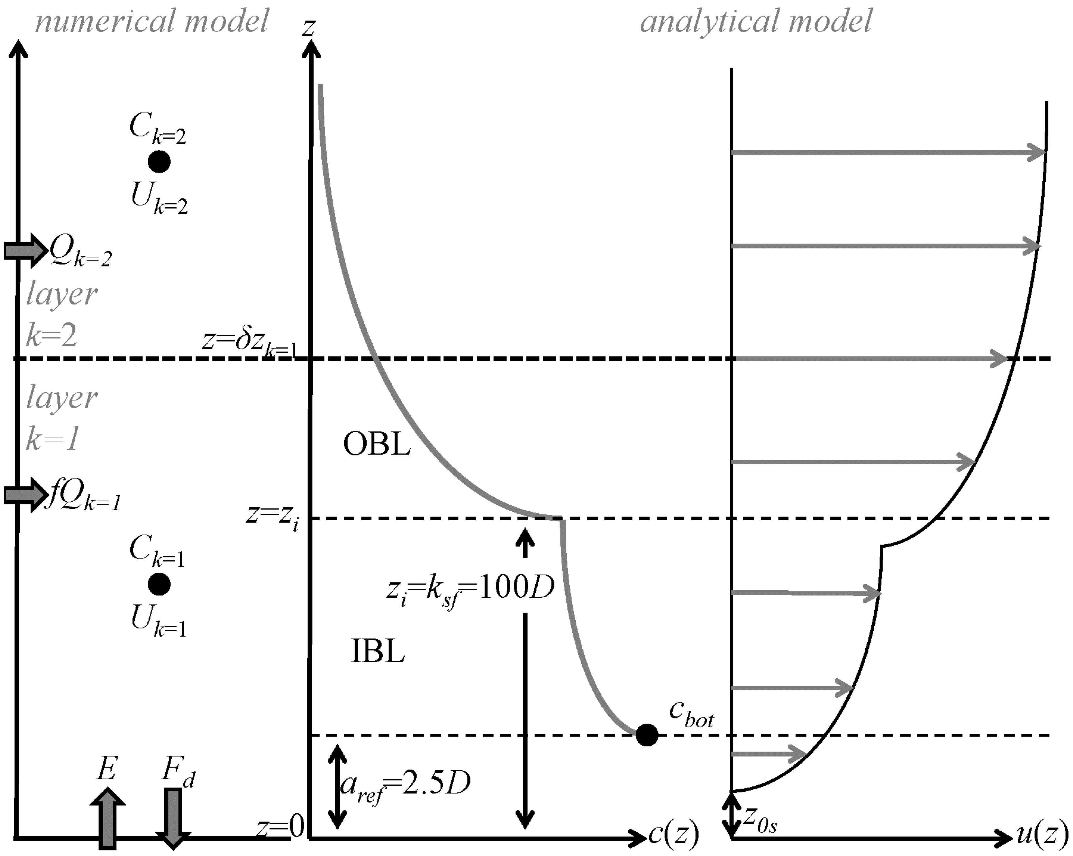
Bottom Boundary Layer Model and Near-Bed Concentration

We follow the concept of the double bottom boundary layer of Smith and Mc Lean [22], which has been found to accurately reproduce the partition between the skin shear stress and the total shear stress [36]. When bed forms are present, the flow is split into two layers above the bottom, the internal boundary layer (IBL), which is controlled by skin roughness, and the outer boundary layer (OBL), which is controlled by bedforms. The velocity profile u(z) in both layers is assumed to follow a logarithmic profile in agreement with the von Karman–Prandtl theory (Figure 1):

$$u(z)=\frac{u_{\ast sf}}{\kappa }ln\left(\frac{z}{z_{0s}}\right) \text{within the IBL}$$

(6)

$$u(z)=\frac{u_{\ast }}{\kappa }ln\left(\frac{z}{z_{0f}}\right) \text{outside the OBL}$$

(7)

where $u_{\ast sf}$ is the friction velocity relative to the IBL, $u_{\ast }$ is the friction velocity relative to the OBL, z_0s the skin roughness (z_0s = k_ss/30 deduced from the grain size; see Appendix A), z_0f the total roughness (z_0f = k_sf/30 deduced from bedform geometry; see Appendix B) and κ the Von Karman constant (= 0.4). It can be noticed that this velocity profile is in agreement with the turbulence closure of the 1DV numerical model (mixing length), but would also have been compatible with other turbulence closures, as most of them are similar in the bottom boundary layer, provided the Reynolds number remains high.

Although the deposition and erosion fluxes may not be balanced, the concentration profile in the bottom layer is assumed to be an equilibrium Rouse profile both inside and outside the IBL (Figure 1). Inside the IBL, vertical mixing is caused by the skin shear stress (${\tau }_{sf}$), whereas it is caused by the total hydraulic shear stress (${\tau }_{ff}$) inside the OBL, so that concentration profiles differ (Figure 1). The method for computing hydraulic shear stress and its skin friction component, under wave and current forcing, is given in Appendix A. Skin roughness z_0s is assumed to only depend on the sediment size, while the form roughness is likely to change in response to the forcing, as the bedform itself depends on the forcing. A bedform predictor is used (Appendix B). When sheet flow is predicted (cf., Appendix B), IBL and OBL merge.

We approximate the IBL thickness (z_i) by the form roughness k_sf (Figure 1). When wave action is important for sediment motion, we assume that the wave boundary layer concerns the whole bottom layer in which the extrapolation is applied. Thus, following Soulsby [1], vertical mixing of sand induced by turbulent wave motion is accounted for by considering the maximum wave + current shear stress during a wave period in the Rouse number expression in both the IBL and the OBL.

The corresponding concentration profile can be written:

- within the IBL ($z<z_i$):

$$c(z)=c_{bot}{\left(\frac{h-z}{z}\frac{a_{ref}}{h-a_{ref}}\right)}^{R_{sf}}$$

(8)

with $c_{bot}=c(a_{ref})$ and the Rouse number within the IBL defined as [1]:

$$R_{sf}=\frac{W_s}{\kappa \sqrt{{\tau }_{sf}/\rho }}$$

(9)

- above the IBL ($z>z_i)$:

$$c(z)=c(z_i){\left(\frac{h-z}{z}\frac{z_i}{h-z_i}\right)}^{R_{ff}}$$

(10)

with c(z_i) computed with Equation (8) for the sake of profile continuity and the Rouse number within the OBL defined as [1]:

$$R_{ff}=\frac{W_s}{\kappa \sqrt{{\tau }_{ff}/\rho }}$$

(11)

Finally, to determine the near-bottom concentration c_bot from the concentration C_{k = 1} computed by the numerical model (Equation (1)) in its bottom layer (k = 1), it is assumed that this concentration is representative of the average concentration within the bottom layer of thickness δz_{k = 1}. The average concentration obtained from the integration of the analytical concentration profile (Equations (8) and (10)) over the bottom layer should then match this representative concentration C_{k = 1} (i.e., ${\displaystyle \underset{a_{ref}}{\overset{\delta z_{k=1}}{\int }}}c(z)dz=C_{k=1}\delta z_{k=1}$). This leads to:

$$c_{bot}=\frac{C_{k=1}\delta z_{k=1}}{a_1{\displaystyle \underset{a_{ref}}{\overset{z_i}{\int }}}{\left(\frac{h-z}{z}\right)}^{R_{sf}}dz+a_2{\displaystyle \underset{z_i}{\overset{\delta z_{k=1}}{\int }}}{\left(\frac{h-z}{z}\right)}^{R_{ff}}dz}$$

(12)

with:

$$a_1={\left(\frac{a_{ref}}{h-a_{ref}}\right)}^{R_{sf}}$$

(13)

and:

$$a_2={\left(\frac{a_{ref}}{z_i}\right)}^{R_{sf}}{\left(\frac{h-z_i}{h-a_{ref}}\right)}^{R_{sf}}{\left(\frac{z_i}{h-z_i}\right)}^{R_{ff}}$$

(14)

2.1.3. Suspended Sediment Horizontal Flux

The transport rate Q_k is calculated by the model in each layer following:

$$Q_k=\frac{1}{{\rho }_s}\delta z_k{U}_k{C}_k$$

(15)

where ρ_s, U_k, C_k and δz_k are respectively the sediment density, the velocity, the sediment concentration and the thickness of the layer k (Figure 1). Note that since the eddy diffusivity is based on the Prandtl mixing length formulation, velocity profile is logarithmic.

Inside the bottom layer, both the velocity profile and suspended concentration profile are subject to large gradients. To account for such gradients, especially when the vertical resolution is low, it is proposed to correct Q₁ in Equation (15). A similar correction procedure has been previously proposed by Waeles et al. [34]. The transport rate thus needs to be corrected to compensate for the low vertical resolution.

The corrected flux can be expressed as $Q_1=\frac{1}{{\rho }_s}f\delta z_{k=1}{U}_{k=1}{C}_{k=1}=\frac{1}{{\rho }_s}{\displaystyle \underset{a_{ref}}{\overset{\delta z_{k=1}}{\int }}}u(z)c(z)dz$ where the corrective factor f for the transport rate is then computed as:

$$f=\frac{{\displaystyle \underset{a_{ref}}{\overset{\delta z_{k=1}}{\int }}}u(z)c(z)dz}{\delta z_{k=1}{U}_{k=1}{C}_{k=1}}$$

(16)

with c(z) defined by Equations (8) and (10) and u(z) defined by Equations (6) and (7) (Figure 1). In Equations (6) and (7), $u_{\ast sf}$and $u_{\ast }$are computed from the velocity U_{k = 1} in the bottom layer (i.e., at z = δz₁/2), ensuring the adequacy of the coupling between the numerical model and the analytical model.

The definite integrals in Equations (12) and (16) are computed using a numerical integration at each time step. For this purpose, the bottom layer is discretised in thin sub-layers (100 sub-layers in this study) with a thickness decreasing toward the bottom to account for the increasing concentration gradient toward the bottom. These numerical integrations require only a little computational work in comparison with the whole model.

2.1.4. Erosion Fluxes

The closure of the model requires that the erosion flux be specified. Several formulations based on experiments are proposed in the literature. However, the horizontal transport rates resulting in fine from those formulations of the erosion flux seem not to have been validated. The validation of sand transport rates using erosion flux formulations will therefore constitute the core of our study.

Non-cohesive sand transport is characterized by a rapidly-reached equilibrium state where the deposition flux balances the erosion flux. Based on Equation (3), when equilibrium is reached, the deposition flux reads:

$$F_d=W_s{c}_a$$

(17)

where c_a represents the so-called reference concentration.

At equilibrium, E = F_d, and the erosion flux can then be expressed as $E=W_s{c}_a$. More generally, some authors propose to express the erosion flux following this latter equation even when equilibrium is not reached (e.g., [24,25,31]). When the erosion boundary condition is expressed with a reference concentration, attention has to be paid to which reference height it refers: naturally, it has to be the same as the one selected for the deposition term.

In this study, four formulations, detailed in Appendix C, were tested. The formulations of Le Hir et al. [23], van Rijn [21], Engelund and Fredsøe [25] and Zyserman and Fredsøe [31] were implemented in the 1DV model and respectively denoted Siam-ERODI, Siam-VR84, Siam-EF76 and Siam-ZF94. In those model configurations, the default reference height (a_ref = 2.5D) was changed to match the reference height corresponding to the erosion boundary condition (if prescribed).

2.2. Transport Rate Validation Strategy

In this section, we present the various data and sand transport rate formulations used to validate the model for different hydrodynamic conditions. All model and data abbreviations are summarized in Table 1.

Table 1. Abbreviations used in this paper for transport models and data. Siam, simulation of multivariate advection; 1DV, one-dimension vertical.

Abbreviations	References
Erosion flux formulations used with Siam 1DV
Siam-ERODI	[23]
Siam-VR84	[21]
Siam-EF76	[25]
Siam-ZF94	[31]
Current only transport formulation
EH67	[37]
Y73	[38]
VR84	[39]
Sediment transport formulations used by Davies et al. [19]
STP	[40]
TKE	[41,42]
BIJKER A	[43,44]
SEDFLUX	[1,45,46]
Dibajnia Watanabe	[47]
TRANSPORT	[48]
Bagnold-Bailard	[49,50]
Sediment transport formulations used by Camenen and Larroudé [51]
Bijker	[52]
Bailard	[50]
van Rijn	[53]
Dibajnia Watanabe	[47]
Ribberink	[54]
Sediment transport data
krammer	[55]
scheldt	[55]
alsalem	[56,57]
janssen	[58]
dibajnia	[47,59]

Table 1. Abbreviations used in this paper for transport models and data. Siam, simulation of multivariate advection; 1DV, one-dimension vertical.

Abbreviations	References
Erosion flux formulations used with Siam 1DV
Siam-ERODI	[23]
Siam-VR84	[21]
Siam-EF76	[25]
Siam-ZF94	[31]
Current only transport formulation
EH67	[37]
Y73	[38]
VR84	[39]
Sediment transport formulations used by Davies et al. [19]
STP	[40]
TKE	[41,42]
BIJKER A	[43,44]
SEDFLUX	[1,45,46]
Dibajnia Watanabe	[47]
TRANSPORT	[48]
Bagnold-Bailard	[49,50]
Sediment transport formulations used by Camenen and Larroudé [51]
Bijker	[52]
Bailard	[50]
van Rijn	[53]
Dibajnia Watanabe	[47]
Ribberink	[54]
Sediment transport data
krammer	[55]
scheldt	[55]
alsalem	[56,57]
janssen	[58]
dibajnia	[47,59]

2.2.1. Current Only

Many practical models that provide the transport rate at equilibrium are proposed in the literature. To validate our model in the case of current only, three well-known formulations of total transport were selected. The expressions of Engelund and Hansen [37], Yang [38] and van Rijn [39], respectively denoted EH67, Y73 and VR84, are detailed in Appendix D. These engineering or practical models (in the sense that they are straightforward computations for sediment transport) were tested by van Rijn [60] for a set of 1260 data acquired in rivers, estuaries and flumes. These experiments were conducted using sand diameters D ranging from 100 to 400 μm and for fluid velocities ranging from 0.4 to 2.4 m/s. According to van Rijn [60], formulations EH67 and VR84 agree relatively well with the data, whereas formulation Y73 underestimates the transport rate in the case of large water height. Moreover, formulations EH67 and Y73 need to determine hydraulic roughness in order to calculate the friction velocity $u_{\star }$, which may considerably modify total transport rates. Calculations using these engineering models (only) are made under flat bed conditions (i.e., the roughness height $k_s=2.5D$ [1]), assuming that no ripples are formed or at least that the required friction velocity is related to skin friction. Formulation VR84 is a simplified method derived from the one proposed by van Rijn [3] in which the hydraulic roughness is not required.

2.2.2. Wave and Current

In order to validate our model in the case of combined wave and current forcing, the results of Davies et al. [19] and Camenen and Larroudé [51] are used. These studies compared transport rates deduced from engineering and research models using a wide range of varying parameters:

$•$ Davies et al. [19] compared several research models (1DV or 2DV) and engineering formulations for a single grain size (250 μm). The same varying roughness $k_s$ is imposed in all of the models according to van Rijn [60]. $k_s$equals 0.1 m for velocities lower than 1 m/s and then decreases almost linearly to reach 0.03 m when current velocity reaches 1.8 m/s. For higher wave conditions (significant wave height H_s > 2 m and wave period T > 7 s) or when the flow velocity reaches 2 m/s, the conditions were considered to correspond to the plane-bed (sheet-flow) regime (i.e., $k_s=2.5D=0.\text{625 mm}$). In our study, we use the results of Davies et al. [19], which include two 1DV models (with high vertical resolution), the STP model [40] and a TKE model [41,42], as well as engineering formulations called BIJKER A [43,44], SEDFLUX [1,45,46], Dibajnia and Watanabe [47], TRANSPORT [48] and Bagnold-Bailard [49,50]. Like in Davies et al. (2002) [19], our model is tested and compared to other models for a set of five hydrodynamic configurations listed in Table 2.

Table 2. Configurations used for the comparison of sediment transport rates computed from various models [19]. Current velocities range between 0 and 2 m/s for each test. Water depth h is fixed (h = 5 m).

Forcing	Hs (m)	T (s)
Current only	0
Current + wave 1	0.5	5
Current + wave 2	1	6
Current + wave 3	2	7
Current + wave 4	3	8

Table 2. Configurations used for the comparison of sediment transport rates computed from various models [19]. Current velocities range between 0 and 2 m/s for each test. Water depth h is fixed (h = 5 m).

Forcing	Hs (m)	T (s)
Current only	0
Current + wave 1	0.5	5
Current + wave 2	1	6
Current + wave 3	2	7
Current + wave 4	3	8

$•$ Camenen and Larroudé [51] compared engineering formulations [47,50,52,53,54] with data for a range of wave conditions (orbital velocity up to 1.7 m/s), current velocities (up to 2.28 m/s), grain size (from 130 to 345 μm) and water levels (from 0.22 to 0.8 m). Most of these experimental data, either from in situ or flume experiments, were acquired under a sheet flow regime. Data from Krammer and Scheldt for beaches (about 120 data, hereafter called krammer and scheldt, respectively) were obtained during strong currents conditions without waves [55]. Laboratory data acquired in oscillating water tunnels with both waves and current (about 260 data) come from Al Salem [56] or from Ribberink and Al Salem [57] (these are called alsalem), from Dohmen-Janssen [58] (called janssen) and from Dibajnia and Watanabee [47] or Dibajnia [59] (called dibajnia). In the present study, the same data are used to validate our model, and the model performance is evaluated using the approach of Camenen and Larroudé [51]. The modelled sediment flux (q_s,num) is considered to be acceptable when it approaches the experimental flux (q_s,data) within a factor 2 (here, “a factor n” means between 1/n times and n times the measured value). For each model, the percentage of values predicted within a factor 2 (i.e., error lower than 50%) and within a factor 1.25 (i.e., error lower than 20%) is computed for “current only” data and “wave-current” data (indicated as Cc50, Cc80, Cw50 and Cw80, respectively). When the experimental flux is negative (current and wave are in opposite directions), the absolute value is shown on the graph if the predicted flux direction is correct. If not, the error is considered to be infinite.

3. Results

The Siam 1DV model described previously was used to simulate equilibrium horizontal transport rates for various erosion flux formulations. In the following section, we evaluate the model results in a simple no-wave configuration.

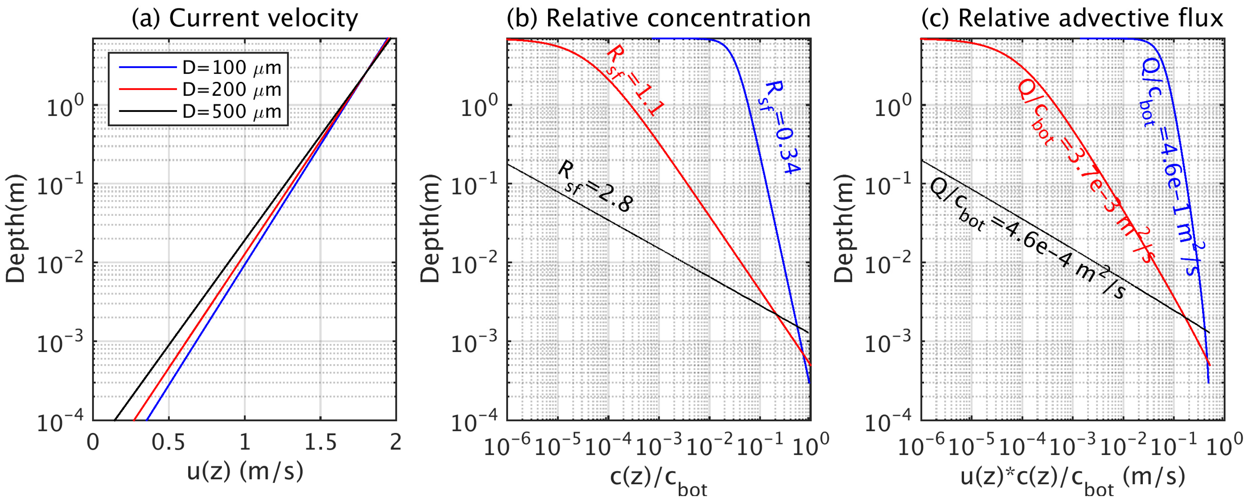
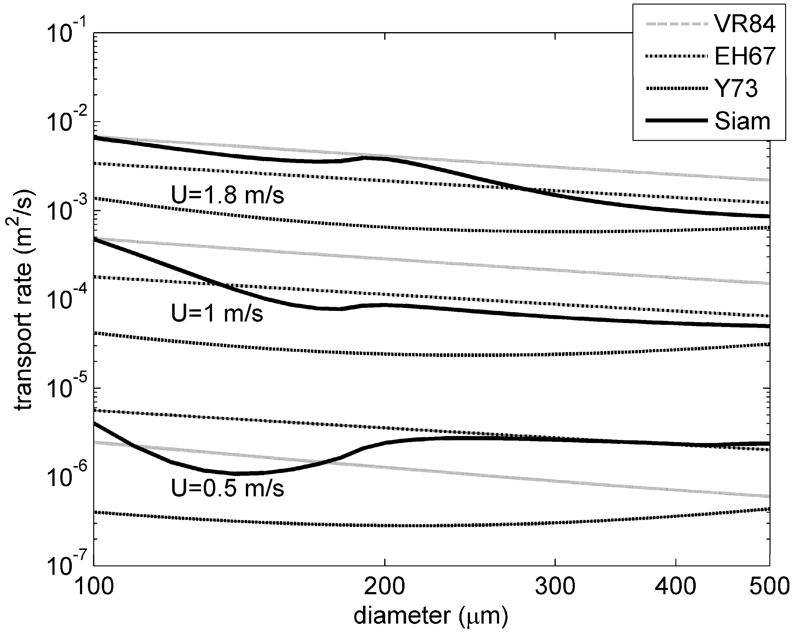
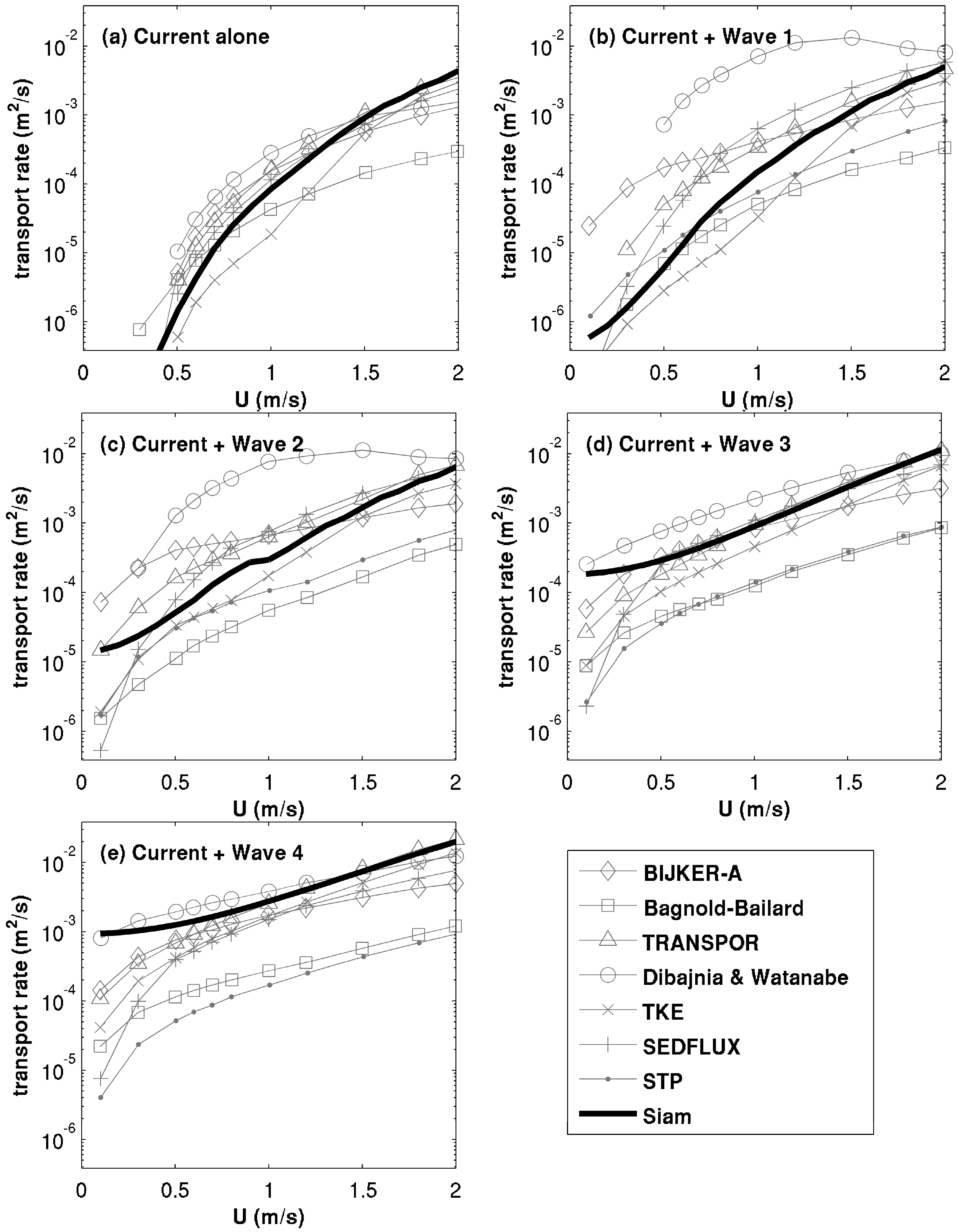
3.1. Evaluation of the 1DV Model Transport Rates in the “Current Only” Case

Results were compared to total transport rates computed with engineering formulations (EH67, Y73 and VR84) and a few data mentioned in the Methods Section. Tests were run for currents varying from 0 to 2 m/s (without waves) and various sand diameters (from 100 to 500 μm) and with a water depth of 7.2 m. The comparison in the case of a current velocity of 1.8 m/s is presented in Figure 2. In agreement with numerous studies, transport rates provided by engineering models differ considerably from one another, as they fluctuate by about one order of magnitude (Figure 2). The few data corresponding to this “current only” experiment fall within the range of values proposed by the three formulations. In agreement with van Rijn [60], formulation Y73 seems to underestimate the transport rate, at least for this particular experiment. Besides, it appears that, whatever erosion flux formulation is used, the transport rates computed by Siam 1DV (hereafter, “1DV transport rates”) do not match the range of engineering and experimental fluxes (Figure 2). Comparisons made for other current velocities (results not shown) confirmed this result. Finer sand fluxes are consistently overestimated, whereas coarser sand fluxes are consistently underestimated.

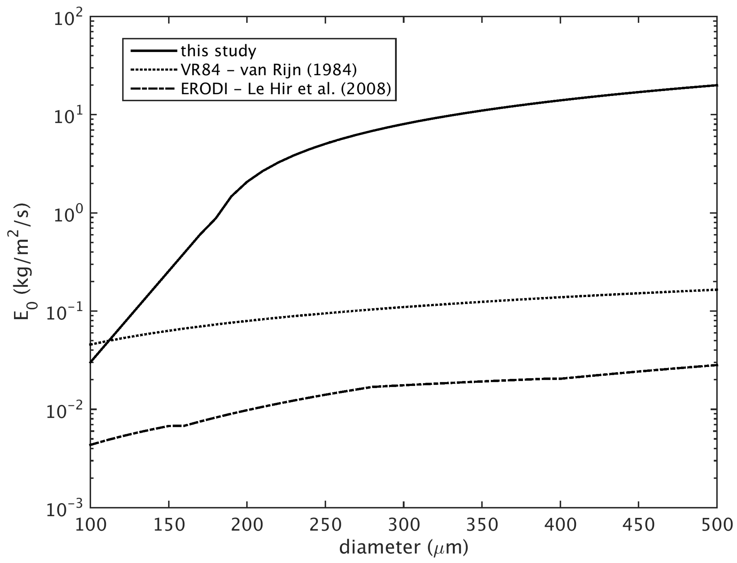
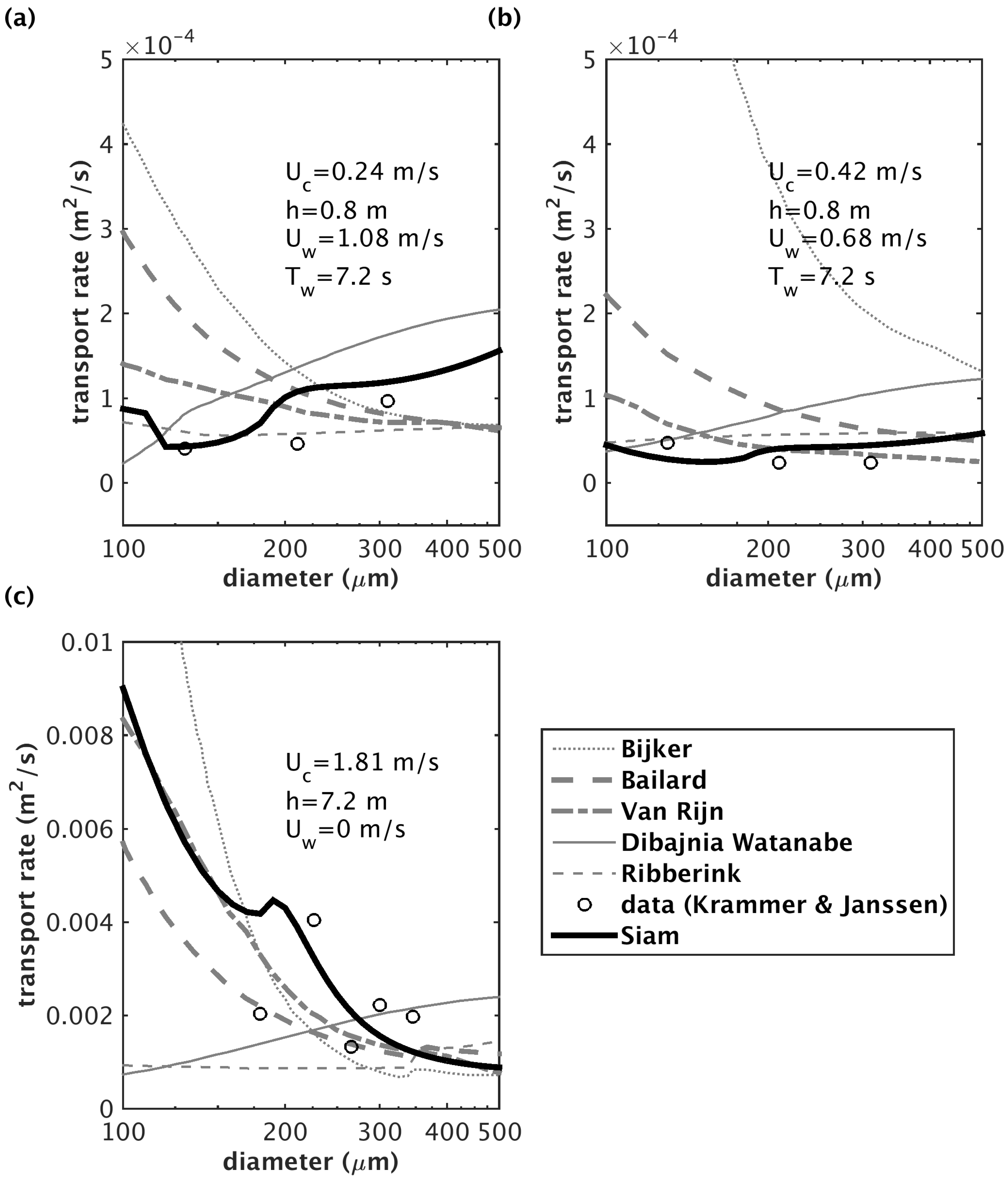
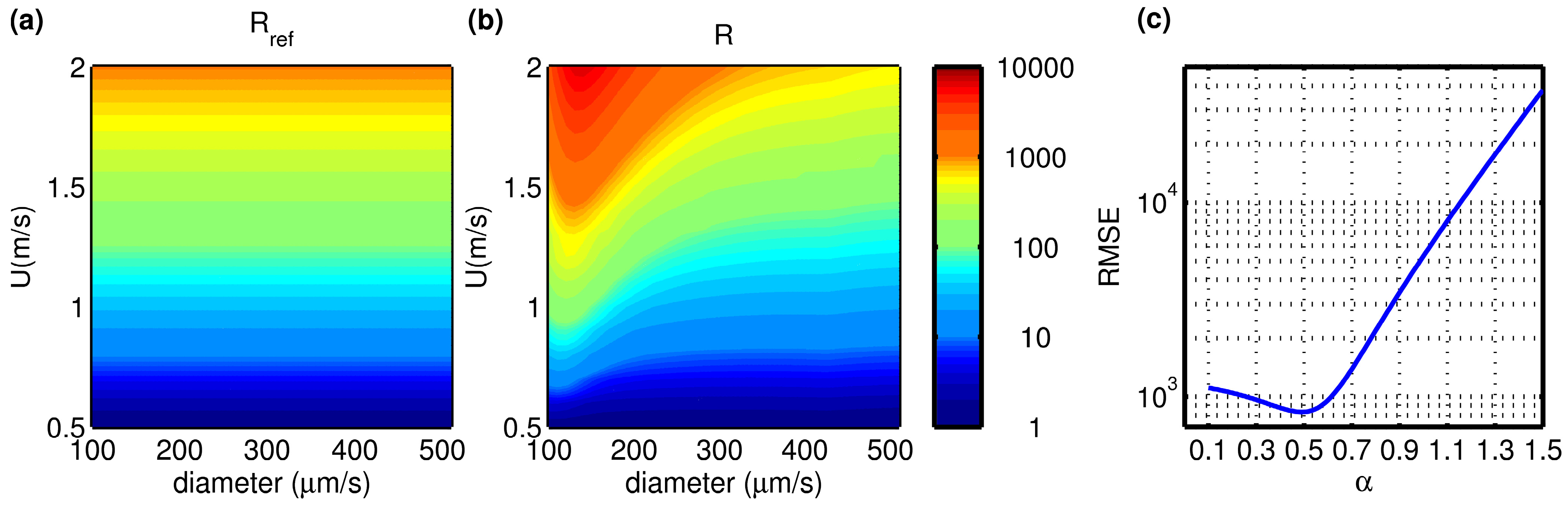
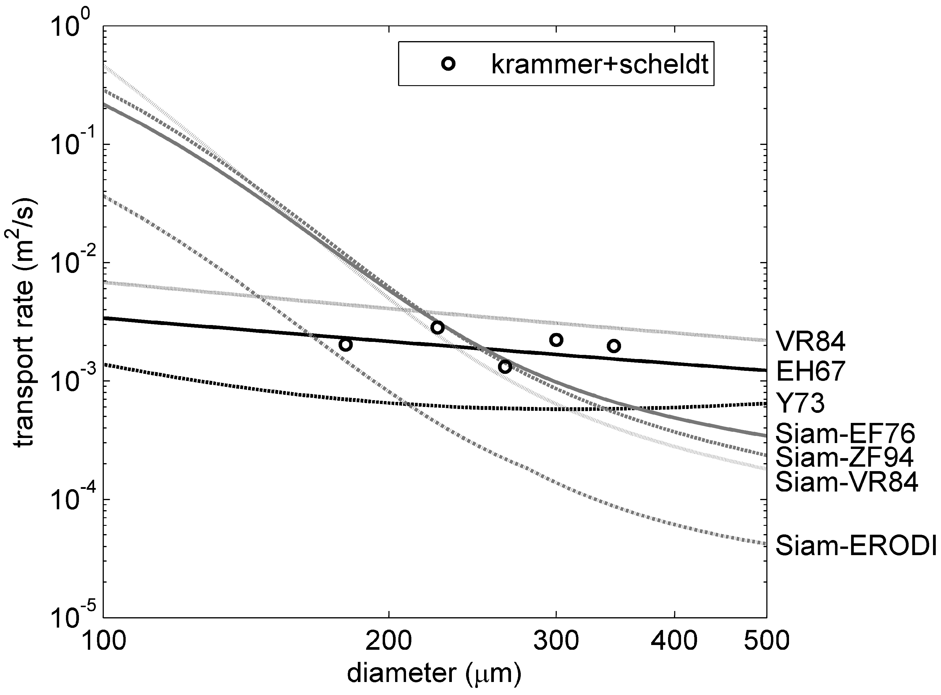
3.2. New Empirical Formulation of Erosion Flux

The previous comparison showed that the erosion fluxes that are given in the literature, after integration by the 1DV model and once equilibrium is reached, lead to largely overestimated horizontal fluxes of fine sand. On the contrary, modelled fluxes are strongly underestimated for coarser sand.

In order to figure out the reason for those discrepancies, we computed the analytical transport rate obtained from the product of a simple Rouse profile (Equation (8)) and a simple logarithmic velocity profile (Equation (6)) in the water column. This test is performed for a mean current velocity of 1.8 m/s and a water depth of 7.2 m (similar to the test in Figure 2). We consider a flat bottom and a_ref = k_sf = 2.5D and z₀ = k_sf/30. The current velocity, the sediment concentration and the transport rate are computed for three grain sizes (100, 200 and 500 μm) and reported in Figure 3.

Figure 2. Sand transport rate as a function of sand diameter for a current velocity of 1.8 m/s. Water depth h is fixed (h = 7.2 m). Engineering models VR84, EH67 and Y73 are tested (black lines). Siam 1DV with different erosion flux formulations (Siam-VR84, Siam-EF76, Siam-ZF94, Siam-ERODI) is also tested (grey lines). Scheldt and krammer data with velocity ranging from 1.8 to 1.84 m/s and h ranging from 6.7 to 7.3 m are added (black circles).

Figure 2. Sand transport rate as a function of sand diameter for a current velocity of 1.8 m/s. Water depth h is fixed (h = 7.2 m). Engineering models VR84, EH67 and Y73 are tested (black lines). Siam 1DV with different erosion flux formulations (Siam-VR84, Siam-EF76, Siam-ZF94, Siam-ERODI) is also tested (grey lines). Scheldt and krammer data with velocity ranging from 1.8 to 1.84 m/s and h ranging from 6.7 to 7.3 m are added (black circles).

Figure 3. Profiles obtained for three different sand sizes, when using a simple logarithmic velocity profile and a Rouse profile for sand concentration. Mean current velocity is 1.8 m/s and water depth h = 7.2 m. (a) Current velocity; (b) relative concentration profile (i.e., concentration normalized by the reference concentration c_bot). The Rouse number R_sf is indicated for each relative concentration profile. (c) Relative transport rate (i.e., transport rate normalized by the reference concentration c_bot). The depth integrated transport rate is indicated next to each profile.

Figure 3. Profiles obtained for three different sand sizes, when using a simple logarithmic velocity profile and a Rouse profile for sand concentration. Mean current velocity is 1.8 m/s and water depth h = 7.2 m. (a) Current velocity; (b) relative concentration profile (i.e., concentration normalized by the reference concentration c_bot). The Rouse number R_sf is indicated for each relative concentration profile. (c) Relative transport rate (i.e., transport rate normalized by the reference concentration c_bot). The depth integrated transport rate is indicated next to each profile.

In this simple configuration, it appears that for the same reference concentration c_bot, the total transport rates for 100 μm and 200 μm sands are two orders of magnitude different (Figure 3). Further, there is only one order of magnitude between the transport rate for 200 μm and 500 μm. According to formulations EH67, VR84 and Y73, transport rates from 100 μm to 500 μm should be within the same order of magnitude (Figure 2). With this simple model, in order to balance the transport rate for the three different grain sizes, a large range of reference concentrations is required, especially between 100 and 200 μm. Since at equilibrium, the erosion flux is proportional to the settling speed, which increases with diameter, and to the reference concentration (E = W_sc_bot), a large dependency of the erosion flux with the diameter is needed. In the erosion flux formulation that we used previously (ERODI and VR84), there is less than one order of magnitude difference from 100 μm to 500 μm (Figure 4). This is likely to explain the discrepancies observed in the Siam 1DV model while using erosion flux formulation from the literature.

Figure 4. Erosion parameter E₀ as a function of sand diameter for several erosion flux formulations. The line labelled “this study” corresponds to Equations (19) and (20). (N.B.: the various orders of magnitude between different formulations are likely to be partly compensated by different powers of the non-dimensional excess shear stress).

Figure 4. Erosion parameter E₀ as a function of sand diameter for several erosion flux formulations. The line labelled “this study” corresponds to Equations (19) and (20). (N.B.: the various orders of magnitude between different formulations are likely to be partly compensated by different powers of the non-dimensional excess shear stress).

Therefore, a new erosion flux has been empirically adjusted. Assuming an erosion law in the form of following Equation (18), we determined the erosion rate in the Siam 1DV that fit the best the range of transport rates calculated with VR84, EH67 and Y73 models for various sand diameters (from 100 to 500 μm) and velocities (from 0 to 2 m/s). More details on the determination of the erosion law are given in Appendix E. The result of the fit leads to the following formulation of the erosion law:

$$E=E_0{\left(\frac{{\tau }_{sf}}{{\tau }_{ce}}-1\right)}^{\alpha }[{\text{kg/m}}^{\text{2}}\text{/s}]$$

(18)

with:

$$E_0={10}^{a_{1}D+b_1}\hspace{1em}\text{if}\hspace{1em}D<180\times {10}^{-6}\text{m}$$

(19)

with a₁ = 18,586 kg·m⁻³·s⁻¹ and b₁ = −3.38 kg·m⁻²·s⁻¹,

and otherwise:

$$E_0=a_{2}D+b_2$$

(20)

with a₂ = 59,658 kg·m⁻³·s⁻¹ and b₂ = −9.86 kg·m⁻²·s⁻¹.

The power law α of the relative excess shear stress is adjusted to 0.5. This empirical formulation involves a coefficient E₀ that depends on the sand diameter (Figure 4). The erosion factor E₀ increases from 0.03 to 21 kg·m⁻²·s⁻¹ for fine sands between 100 and 500 μm. The critical shear stress τ_ce is computed from the classical critical Shields’ parameter for sand movement.

3.3. Validation of the New Erosion Flux Formulation

The result of the fit that led to the formulation of the erosion law is presented in Figure 5 for three different velocities (0.5, 1 and 1.8 m/s). The transport rates obtained with the new erosion flux formulation match well with the engineering formulations VR84, EH67 and Y73 in the case of current only. In the following sections, we further assess the capacity of the model to transport sand in suspension for a range of different configurations.

Figure 5. Transport rate as a function of sand diameter for three current velocity configurations (grey areas). Engineering models VR84, EH67 and Y73 and the 1DV model (Siam) using the new erosion law (Equations (18)–(20)) are tested.

Figure 5. Transport rate as a function of sand diameter for three current velocity configurations (grey areas). Engineering models VR84, EH67 and Y73 and the 1DV model (Siam) using the new erosion law (Equations (18)–(20)) are tested.

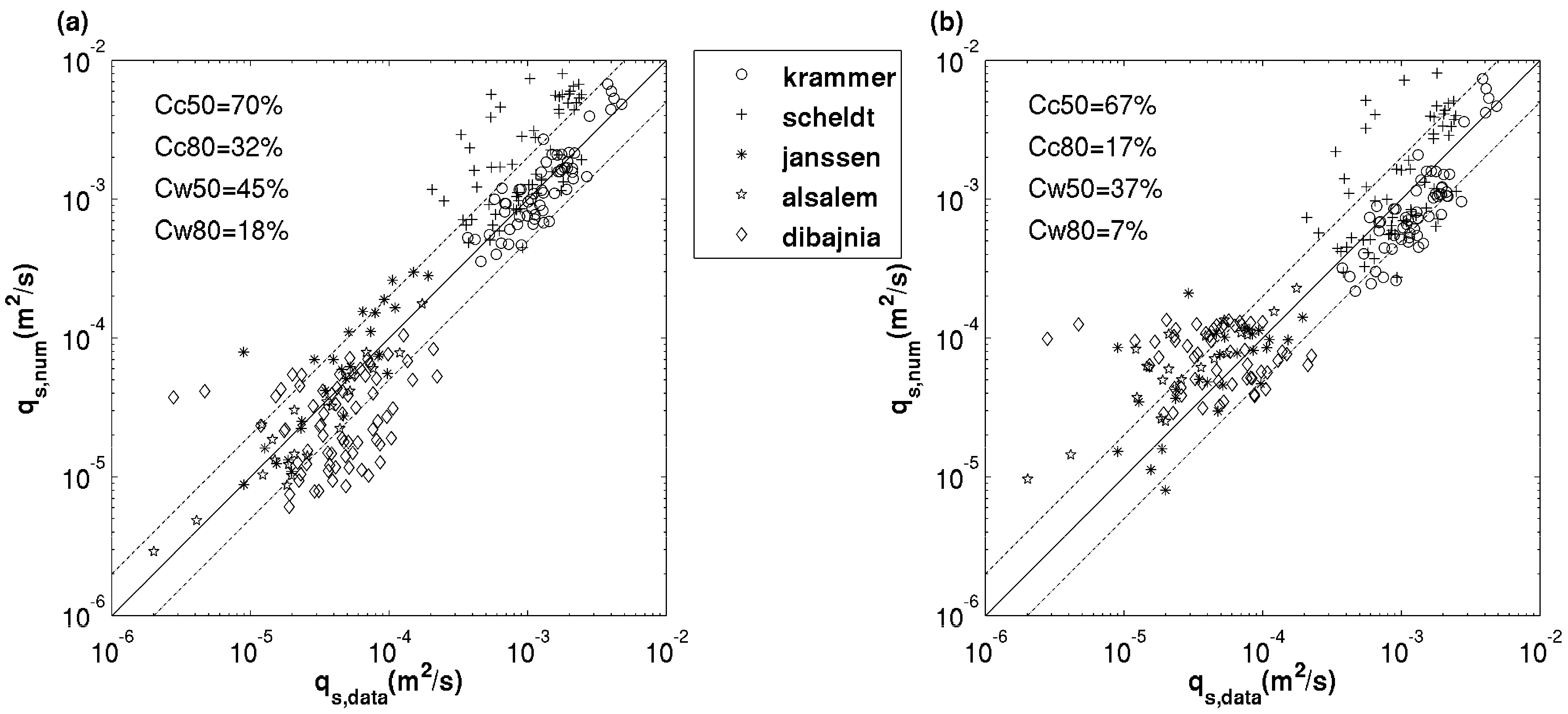
3.3.1. Overall Performance

For the purpose of comparison, Figure 6a shows the results obtained by Camenen and Larroudé [51] with the van Rijn [53] formulation, which is considered to yield reasonable results (Camenen and Larroudé [51]). According to Figure 6b, the transport rates computed with the advection/diffusion model and our erosion law (Equations (18)–(20)) compare reasonably well with the empirical laws used to directly assess equilibrium solid fluxes. Measured transport rates were predicted within a factor 2 in 67% of cases with current only and in 35% of cases with both waves and current (Table 3). However, an overestimation is sometimes observed in the case of the scheldt data (concerning strong currents and fine sands). Under wave-current interaction, the model also overestimates data sometimes. A considerable error is likely to appear when waves become strongly asymmetric, as the model was not designed to account for the aforementioned process. Actually, at least one third of the data corresponding to wave forcing was acquired under asymmetric waves, inducing significant transport rates without current or transport opposite the current direction.

Table 3. Comparison between various models and data described by Camenen and Larroudé [51] and in this study. See the explanations of symbols Cc and Cw in the Methods Section. Adapted from Camenen and Larroudé [51].

Model	Cc50: Current only	Cw50: Wave + Current
Bijker [52]	66	18
Bailard [50]	82	35
van Rijn [53]	70	45
Dibajnia Watanabe [47]	84	48
Ribberink [54]	60	45
Siam 1DV + erosion law (this paper)	67	37

Table 3. Comparison between various models and data described by Camenen and Larroudé [51] and in this study. See the explanations of symbols Cc and Cw in the Methods Section. Adapted from Camenen and Larroudé [51].

Model	Cc50: Current only	Cw50: Wave + Current
Bijker [52]	66	18
Bailard [50]	82	35
van Rijn [53]	70	45
Dibajnia Watanabe [47]	84	48
Ribberink [54]	60	45
Siam 1DV + erosion law (this paper)	67	37

Figure 6. (a) Comparison of total sand transport rates between the Van Rijn [53] formula (q_s,num) and experimental data (q_s,data). From Camenen and Larroudé [51]. (b) Comparison of total sand transport rates between Siam 1DV (q_s,num) and experimental data (q_s,data). See the explanations of the legend and symbols Cc and Cw in the Methods Section. Values predicted within a factor 2 sit in between the two dashed lines (q_s,num = 0.5q_s,data and q_s,num = 2q_s,data).

Figure 6. (a) Comparison of total sand transport rates between the Van Rijn [53] formula (q_s,num) and experimental data (q_s,data). From Camenen and Larroudé [51]. (b) Comparison of total sand transport rates between Siam 1DV (q_s,num) and experimental data (q_s,data). See the explanations of the legend and symbols Cc and Cw in the Methods Section. Values predicted within a factor 2 sit in between the two dashed lines (q_s,num = 0.5q_s,data and q_s,num = 2q_s,data).

Figure 7. Comparison of sand transport rates as a function of sand diameter in the case of prevailing waves (a); the case of wave and current (b) and the case of current only (c). Bold black curves, corresponding to Siam 1DV transport rates using the new erosion law (Equations (18)–(20)), are added to other models’ results (copied from Camenen and Larroudé [51]). U_c is the mean current velocity; h the water depth; T_w is the wave period; and U_w is the wave orbital velocity at the bottom.

Figure 7. Comparison of sand transport rates as a function of sand diameter in the case of prevailing waves (a); the case of wave and current (b) and the case of current only (c). Bold black curves, corresponding to Siam 1DV transport rates using the new erosion law (Equations (18)–(20)), are added to other models’ results (copied from Camenen and Larroudé [51]). U_c is the mean current velocity; h the water depth; T_w is the wave period; and U_w is the wave orbital velocity at the bottom.

3.3.2. Validation for Varying Grain Size

The effect of grain size variation was investigated with the Siam 1DV approach, and results were added to the comparison of Camenen and Larroudé [51] (Figure 7). Results are coherent with both data and other transport rate formulations in the case of prevailing waves, waves and current or prevailing current (Figure 7). The large disparities in transport rates for finer sands highlight the difficulty in validating the model for fine sands. This is due to the fact that most studies focus on sand around 200 μm [51]. Other parameters (wave orbital velocity, wave period, current) were also tested, and the resulting transport rates showed good agreement with the results of Camenen and Larroudé [51] (results not shown).

Figure 8. Comparison of sand transport rates for different wave and current conditions (cf., Table 2) (sand diameter 250 μm). Bold black curves, corresponding to Siam 1DV transport rates using the new erosion law (Equations (18)–(20)), are added to other models’ results (copied from Davies et al. [19]).

Figure 8. Comparison of sand transport rates for different wave and current conditions (cf., Table 2) (sand diameter 250 μm). Bold black curves, corresponding to Siam 1DV transport rates using the new erosion law (Equations (18)–(20)), are added to other models’ results (copied from Davies et al. [19]).

3.3.3. Validation for Varying Hydrodynamic Conditions

The robustness of the model for a wide range of wave and current conditions was finally checked by adding Siam 1DV results to the comparison study presented by Davies et al. [19] (Figure 8). These comparisons confirmed the good behaviour of the model for different hydrodynamic conditions. However, in the case of strong waves, the Siam model provides among the highest transport rates of the comparison. This matches with the previous comparison with data that showed a slight overestimation in the case of waves (Figure 6b).

3.4. Relevance of Analytical Refinements in the Bottom Layer

We tested the impact of the vertical resolution on the transport rate. First, we used the model without either extrapolating the near bed concentration from the model concentration in the bottom layer (for deposition) or correcting the expression of horizontal flux in the bottom layer (i.e., f = 1 and F_d = W_sC_{k = 1}). In this configuration, the sand fluxes in the case of current only are highly dependent on the vertical resolution (Figure 9). For two different resolutions of the bottom layer (20 cm and 5 m), the transport rates (grey lines) vary by about one order of magnitude. On the contrary, transport rates calculated with the model presented in this study are nearly independent of the resolution of the model (Figure 9). We can however note that some discontinuities, related to the appearance of the sheet-flow regime, are encountered. The change of roughness under sheet-flow and its impact on the suspended flux depend on the model resolution in our model.

Figure 9. Siam 1DV sand transport rates for current only with varying velocity (sand diameter 200 μm, water depth h = 10 m). Several configurations of the model are tested. The resolution of the bottom layer k = 1 is 20 cm for the solid line and 5 m for the dotted line. The results of the model presented in this study are in black. The results of the numerical model without analytical refinement in the bottom layer (i.e., f = 1 and F_d = W_sC_{k = 1}) are in grey.

Figure 9. Siam 1DV sand transport rates for current only with varying velocity (sand diameter 200 μm, water depth h = 10 m). Several configurations of the model are tested. The resolution of the bottom layer k = 1 is 20 cm for the solid line and 5 m for the dotted line. The results of the model presented in this study are in black. The results of the numerical model without analytical refinement in the bottom layer (i.e., f = 1 and F_d = W_sC_{k = 1}) are in grey.

4. Discussion

We tested the model, using several erosion flux formulations from the literature, against data and equilibrium transport rate formulations. None of these erosion flux formulations tested in the model led to acceptable simulations of sand transport rates. Three hypotheses could be suggested to explain this inconsistency:

• Bed load has not been accounted for in our model. For the experiment leading to Figure 2, adding the bed load in the model leads to the same conclusion. For instance, using VR84, which gives both suspended load and bed load, it appears that, whatever the velocity, the bed load only accounts for 6%–22% of the total transport from the finer to the coarser sand (following VR84, the ratio of the suspended load to the total load is independent of the velocity). Moreover, for the “current only” experiment (Figure 2), the ratio $u_{\ast }/W_s$ is always greater than one, which means that the suspended load is the predominant mode of transport [61]. The bed load is therefore not expected to explain the discrepancies observed when using classical erosion flux formulations, at least for this experiment.
• The 1DV model could suffer from weaknesses, mostly in the way the boundary layer is formulated. It is for instance not fully clear if the Rouse profile holds very close to the bottom. Different tests were conducted with varying parameterization (reference height, hindered settling velocity or the parameterization of vertical mixing were modified) and led to the same conclusion. A simple Rouse concentration profile (assuming a single bottom boundary layer) has also been tested, but did not enable us to match the total flux range given by engineering models. Further, we cannot take into account the impact of sediment concentration on settling velocity near the bottom in the model. This is due to the fact that we are using an analytical solution for the bottom layer of the model (a Rouse profile), which is only valid for constant settling velocity (with depth). We acknowledge that this could induce biases in the transport rates computed by the model.
• The erosion fluxes proposed in the literature could be inconsistent with our modelling strategy. We suggest here that this hypothesis is the most relevant one. Our approach was thus to search for an empirical erosion law able to produce results that match the horizontal flux range given by empirical engineering models.

The ability to transport sand with an advection-diffusion equation was then achieved by introducing a new empirical erosion law. It should be noted that this erosion law is consistent with a reference height (elevation where the deposition flux is evaluated) of 2.5D. The erosion flux involves a power law of the excess shear stress multiplied by a nonlinear function of the sand diameter. The power α of 0.5 is in agreement with the formulation proposed by Waeles et al. [13], but is lower than in other classical formulations [21,23]. We tested different power α, in agreement with other formulations [21,23], but this did not lead to acceptable results. Indeed, in Figure 8a, for instance, the shape of the curve was not matching the expected shape, with a much steeper increase of the transport rate with current velocity than expected. The variation of E₀ with D is much more amplified than in other formulations (Figure 4). We acknowledge that this erosion flux formulation may be dependent on the conceptual model of the boundary layer that we adopted in this study. Transposing this erosion flux formulation to other studies would therefore require using the same boundary layer conceptual model. However, we suggest that the strong variation of E₀ with D is not specific to our model and that the same behaviour would be observed for any other comparable model. This aspect would require further investigations. We also suggest that the same validation approach should be carried out when using multi-class sediment transport models using advection-diffusion equations for sand. Further, due to the strong variation of E₀ with D and the discontinuity in the formulation around 180 μm, we acknowledge that some discontinuities in the transport rates can be produced (e.g., Figure 7c). This, however, should not be an issue for implementation in 3D models using a discrete form of E₀ (i.e., using only a few sand classes).

In this study, we looked at transport rates at equilibrium, so that the coupling between an unsteady numerical model and a stationary analytical model remains coherent. Further investigations should, however, be carried out to evaluate the impact of this coupling while studying unsteady flows. We also acknowledge that, since the model does not account for bed load, it has been validated for medium sands, probably thanks to some compensation in the fitted erosion law. If our approach seems reasonable in the case of fine sand particles, it would probably reach its own limit when the bed load is prevailing.

The strength of the 1DV approach compared to engineering or practical models is that it computes the sediment concentration profile in the whole water column. In the present study, we only validated the total sediment transport at equilibrium. In the future, it would also be interesting to compare the sediment concentration profile with field data, especially close to the sediment bed, where the analytical model is coupled, and in non-stationary conditions.

In parallel with the validation of the suspended sediment transport model at equilibrium (this study), the model was implemented in a 3D multi-class sediment transport model [12]. It was tested at shelf scale using one class of mud and two classes of sand (160 and 380 μm). For the sand fractions, the erosion flux formulation and the conceptual model of the boundary layer presented in this study were adopted, and the sediment dynamics in that modelling study proved to be consistent with in situ measurements [12].

5. Conclusions

Transporting sand in suspension is necessary in sediment transport models dealing with cohesive sediment, in order to allow the management of mixtures of sand and mud. The initial objective of this work was to evaluate the ability to predict fine to medium sand horizontal fluxes under varying wave and current conditions by using an advection-diffusion model. It has been shown that using classical erosion rate formulations from the literature in our model did not lead to consistent results. Those classical erosion laws should not be used in advection-diffusion models without a full validation procedure involving a range of sand diameters and hydrodynamic conditions. The ability to transport fine sands in our modelling framework was only made possible by introducing a new empirical erosion law. Further, the transport rate computed from the advection-diffusion model had to be independent of the vertical resolution, so that it can be implemented in regional models with operational applications. This was successfully achieved by using a correction procedure for extrapolating the near-bed concentration (in the deposition flux) from the concentration computed in the bottom layer. In addition, the actual horizontal flux in this bottom layer deserved a correction to account for very strong inverse gradients of velocity and concentration in the boundary layer. It is suggested that in a three-dimensional model, such a flux correction should be applied when solving the advection-diffusion equation for suspensions.

Using the new empirical erosion flux formulation, the model demonstrated its capacity to simulate transport rates for sand diameter in the range 100–500 μm. The proposed erosion law was evaluated as best as possible for a wide range of different hydrodynamic conditions and grain sizes. This has been done despite the difficulty involved in qualifying sand transport models, illustrated by the very scattered results of classical sand transport formulations [19,41,51,60,62]. This evaluation showed that our model compares well with various other sand transport models. While comparing the model with data, we showed that measured transport rates were predicted within a factor 2 in 67% of cases with current only and in 35% of cases with both waves and current. In comparison with the results obtained by Camenen and Larroudé [51], who provided the same indicators for several practical transport rate formulations (whose means are respectively 72% and 37%), our model gives reasonable results.

Finally, the model presented in this study has been formulated for well-sorted, non-cohesive sediments. In the future, it would have to be adapted in the case of heterogeneous sediment composition to reach our longer term goal.

References

1. Soulsby, R.L. Dynamics of Marine Sands. A Manual for Practical Applications; Thomas Telford: London, UK, 1997; p. 249. [Google Scholar]
2. Whitehouse, R.; Soulsby, R.L.; Roberts, W.; Mitchener, H. Dynamics of Estuarine Muds; Thomas Telford: London, UK, 2000; p. 210. [Google Scholar]
3. Van Rijn, L.C. Sediment transport: Part I: Bed load transport. J. Hydraul. Ing. Proc. Am. Soc. Civ. Eng. 1984, 110, 1431–1456. [Google Scholar] [CrossRef]
4. Einstein, H. The Bed-Load Function for Sediment Transportation in Open Channel Flows; United States Department of Agriculture, Soil Conservation Services: Washington, DC, USA, 1950.
5. Meyer-Peter, E.; Müller, R. Formulas for Bed-Load Transport. In Proceedings of the 2nd Meeting of the International Association for Hydraulic Structure Research, Stockholm, Sweden, 7–9 June 1948; pp. 39–64.
6. Mitchener, H.; Torfs, H. Erosion of mud/sand mixtures. Coast. Eng. 1996, 29, 1–25. [Google Scholar] [CrossRef]
7. Panagiotopoulos, I.; Voulgaris, G.; Collins, M.B. The influence of clay on the threshold of movement of fine sandy beds. Coast. Eng. 1997, 32, 19–43. [Google Scholar] [CrossRef]
8. Migniot, C. Tassement et rhéologie des vases—Première partie. Houille Blanche 1989, 1, 11–29. [Google Scholar] [CrossRef]
9. Van Ledden, M.; Wang, Z.B. Sand-Mud Morphodynamics in an Estuary. In Proceedings of the 2nd Symposium on River, Coastal and Estuarine Morphodynamics, Obihiro, Japan, 10–14 September 2001; pp. 505–514.
10. Chesher, T.J.; Ockenden, M. Numerical modelling of mud and sand mixture. In Cohesive Sediments; John Wiley & Sons: New York, NY, USA, 1997; pp. 395–406. [Google Scholar]
11. Le Hir, P.; Cayocca, F.; Waeles, B. Dynamics of sand and mud mixtures: A multiprocess-based modelling strategy. Cont. Shelf Res. 2011, 31, S135–S149. [Google Scholar] [CrossRef]
12. Dufois, F.; Verney, R.; Le Hir, P.; Dumas, F.; Charmasson, S. Impact of winter storms on sediment erosion in the rhone river prodelta and fate of sediment in the gulf of lions (north western mediterranean sea). Cont. Shelf Res. 2014, 72, 57–72. [Google Scholar] [CrossRef]
13. Waeles, B.; Le Hir, P.; Lesueur, P. A 3D morphodynamic process-based modelling of a mixed sand/mud coastal environment: The seine estuary, France. Proc. Mar. Sci. 2008, 9, 477–498. [Google Scholar]
14. Sanford, L.P. Modeling a dynamically varying mixed sediment bed with erosion, deposition, bioturbation, consolidation, and armoring. Comput. Geosci. 2008, 34, 1263–1283. [Google Scholar] [CrossRef]
15. Van Ledden, M. A process-based sand-mud model. Proc. Mar. Sci. 2002, 5, 577–594. [Google Scholar]
16. Harris, C.K.; Wiberg, P.L. A two-dimensional, time-dependent model of suspended sediment transport and bed reworking for continental shelves. Comput. Geosci. 2001, 27, 675–690. [Google Scholar] [CrossRef]
17. Ulses, C.; Estournel, C.; Durrieu de Madron, X.; Palanques, A. Suspended sediment transport in the gulf of lion (NW mediterranean): Impact of extreme storms and floods. Cont. Shelf Res. 2008, 28, 2048–2070. [Google Scholar] [CrossRef]
18. Sherwood, C.R.; Book, J.W.; Carniel, S.; Cavaleri, L.; Chiggiato, J.; Das, H.; Doyle, J.D.; Harris, C.K.; Niedoroda, A.W.; Perkins, H.; et al. Sediment dynamics in the Adriatic sea investigated with coupled models. Oceanography 2004, 17, 58–69. [Google Scholar] [CrossRef]
19. Davies, A.G.; van Rijn, L.C.; Damgaard, J.S.; van de Graaff, J.; Ribberink, J.S. Intercomparison of research and practical sand transport models. Coast. Eng. 2002, 46, 1–23. [Google Scholar] [CrossRef]
20. Waeles, B. Modélisation Morphodynamique de L’embouchure de la Seine. Ph.D. Thesis, Université de Caen, Caen, France, 2005. [Google Scholar]
21. Van Rijn, L.C. Sediment pick-up functions. J. Hydraul. Eng. 1984, 110, 1494–1502. [Google Scholar] [CrossRef]
22. Smith, J.D.; McLean, S.R. Spatially averaged flow over a wavy surface. J. Geophys. Res. 1977, 82, 1735–1746. [Google Scholar] [CrossRef]
23. Le Hir, P.; Cann, P.; Waeles, B.; Jestin, H.; Bassoulet, P. Erodibility of natural sediments: Experiments on sand/mud mixtures from laboratory and field erosion tests. Proc. Mar. Sci. 2008, 9, 137–153. [Google Scholar]
24. Van Rijn, L.C. Sediment transport: Part II: Suspended load transport. J. Hydraul. Ing. Proc. Am. Soc. Civ. Eng. 1984, 110, 1613–1641. [Google Scholar] [CrossRef]
25. Engelund, F.; Fredsøe, J. A sediment transport model for straight alluvial channels. Nord. Hydrol. 1976, 7, 293–306. [Google Scholar]
26. Nielsen, P. Coastal Bottom Boundary Layers and Sediment Transport; World Scientific: Singapore, Singapore, 1992; p. 324. [Google Scholar]
27. Lesser, G.; Roelvink, J.; Van Kester, J.; Stelling, G. Development and validation of a three-dimensional morphological model. Coast. Eng. 2004, 51, 883–915. [Google Scholar] [CrossRef]
28. Papanicolaou, A.N.; Elhakeem, M.; Krallis, G.; Prakash, S.; Edinger, J. Sediment transport modeling review—Current and future developments. J. Hydraul. Eng. 2008, 134, 1–14. [Google Scholar] [CrossRef]
29. Villaret, C.; Hervouet, J.-M.; Kopmann, R.; Merkel, U.; Davies, A.G. Morphodynamic modeling using the telemac finite-element system. Comput. Geosci. 2013, 53, 105–113. [Google Scholar] [CrossRef]
30. Warner, J.C.; Sherwood, C.R.; Signell, R.P.; Harris, C.K.; Arango, H.G. Development of a three-dimensional, regional, coupled wave, current, and sediment-transport model. Comput. Geosci. 2008, 34, 1284–1306. [Google Scholar] [CrossRef]
31. Zyserman, J.A.; Fredsøe, J. Data analysis of bed concentration of suspended sediment. J. Hydraul. Eng. 1994, 120, 1021–1042. [Google Scholar] [CrossRef]
32. Le Hir, P.; Ficht, A.; Jacinto, R.S.; Lesueur, P.; Dupont, J.-P.; Lafite, R.; Brenon, I.; Thouvenin, B.; Cugier, P. Fine sediment transport and accumulations at the mouth of the seine estuary (France). Estuaries 2001, 24, 950–963. [Google Scholar] [CrossRef]
33. Brenon, I.; Le Hir, P. Modelling the turbidity maximum in the seine estuary (France): Identification of formation processes. Estuar. Coast. Shelf Sci. 1999, 49, 525–544. [Google Scholar] [CrossRef]
34. Waeles, B.; Le Hir, P.; Lesueur, P.; Delsinne, N. Modelling sand/mud transport and morphodynamics in the seine river mouth (France): An attempt using a process-based approach. Hydrobiologia 2007, 588, 69–82. [Google Scholar] [CrossRef]
35. Reed, C.W.; Niedoroda, A.W.; Swift, D.J. Modeling sediment entrainment and transport processes limited by bed armoring. Mar. Geol. 1999, 154, 143–154. [Google Scholar] [CrossRef]
36. Li, Z. Direct skin friction measurements and stress partitioning over movable sand ripples. J. Geophys. Res. Ocean. (1978–2012) 1994, 99, 791–799. [Google Scholar]
37. Engelund, F.; Hansen, A. A Monograph on Sediment Transport in Alluvial Streams; Verlag Technik: Copenhagen, Denmark, 1967; p. 62. [Google Scholar]
38. Yang, C. Incipient motion and sediment transport. J. Hydraul. Div. Proc. Am. Soc. Civ. Eng. 1973, 99, 1679–1703. [Google Scholar]
39. Van Rijn, L.C. Sediment transport: Part III: Bed forms and alluvial roughness. J. Hydraul. Ing. Proc. Am. Soc. Civ. Eng. 1984, 110, 1733–1754. [Google Scholar] [CrossRef]
40. Fredsøe, J.; Andersen, O.H.; Silberg, S. Distribution of suspended sediment in large waves. J. Waterw. Port Coast. Ocean Eng. 1985, 111, 104–1059. [Google Scholar] [CrossRef]
41. Davies, A.G.; Villaret, C. Sand Transport by Waves and Currents: Predictions of Research and Engineering Models. In Proceedings of the 27th International Conference on Coastal Engineering, Sydney, Australia, ASCE, 16–21 July 2000; pp. 2481–2494.
42. Davies, A.G.; Li, Z. Modelling sediment transport beneath regular symmetrical and asymmetrical waves above a plane bed. Cont. Shelf Res. 1997, 17, 555–582. [Google Scholar] [CrossRef]
43. Bijker, E.W. Longshore transport computations. J. Waterw. Harb. Coast. Eng. Div. 1971, 97, 687–701. [Google Scholar]
44. Bijker, E.W. Mechanics of Sediment Transport by the Combination of Waves and Current. In Proceedings of the 23rd International Conference on Coastal Engineering—Design and Reliability of Coastal Structures, Venice, Italy, ASCE, 1–3 October 1992; pp. 147–173.
45. Damgaard, J.S.; Stripling, S.; Soulsby, R.L. Numerical Modelling of Coastal Shingle Transport; HR Wallingford: Wallingford, UK, 1996. [Google Scholar]
46. Damgaard, J.S.; Hall, L.J.; Soulsby, R.L. General engineering sand transport model: Sedflux. In Sediment Transport Modelling in Marine Coastal Environments; van Rijn, L.C., Davies, A.G., van de Graaff, J., Ribberink, J.S., Eds.; Aqua Publications: Amsterdam, The Nederlands, 2001. [Google Scholar]
47. Dibajnia, M.; Watanabe, A. Sheet Flow under Nonlinear Waves and Currents. In Proceedings of the 23rd International Conference on Coastal Engineering, Venice, Italy, ASCE, 1–3 October 1992; pp. 2015–2028.
48. Van Rijn, L.C. General View on Sand Transport by Currents and Waves; Delft Hydraulics: Delft, The Netherlands, 2000. [Google Scholar]
49. Bagnold, R.A. An approach to the sediment transport problem from general physics. U.S. Geol. Surv. 1966, 442, 37. [Google Scholar]
50. Bailard, J.A. An energetics total load sediment transport model for plane sloping beach. J. Geophys. Res. 1981, 86, 10938–10954. [Google Scholar] [CrossRef]
51. Camenen, B.; Larroudé, P. Comparison of sediment transport formulae for the coastal environment. Coast. Eng. 2003, 48, 111–132. [Google Scholar] [CrossRef]
52. Bijker, E.W. Littoral Drift as Function of Waves and Current. In Proceedings of the 11th International Conference on Coastal Engineering, London, UK, ASCE, September 1968; pp. 415–435.
53. Van Rijn, L.C. Handbook Sediment Transport by Currents and Waves; Delft Hydraulics: Delft, The Netherlands, 1989. [Google Scholar]
54. Ribberink, J. Bed-load transport for steady flows and unsteady oscillatory flows. Coast. Eng. 1998, 34, 59–82. [Google Scholar] [CrossRef]
55. Voogt, L.; van Rijn, L.C.; van den Berg, J.H. Sediment transport of fine sands at high velocities. J. Hydraul. Eng. 1991, 117, 869–890. [Google Scholar] [CrossRef]
56. Al Salem, A. Sediment Transport in Oscillatory Boundary Layers under Sheet Flow Conditions. Ph.D. Thesis, Delft Hydraulics, The Netherlands, 1993. [Google Scholar]
57. Ribberink, J.; Al Salem, A. Sediment transport in oscillatory boundary layers in cases of rippled beds and sheet flow. J. Geophys. Res. 1994, 99, 707–727. [Google Scholar] [CrossRef]
58. Dohmen-Janssen, M. Grain Size Influence on Sediment Transport in Oscillatory Sheet Flow, Phase-Lags and Mobile-Bed Effects. PhD Thesis, Delft University of Technology, Delft, The Netherlands, 1999. [Google Scholar]
59. Dibajnia, M. Sheet flow transport formula extended and applied to horizontal plane problems. Coast. Eng. Jpn. 1995, 38, 178–194. [Google Scholar]
60. Van Rijn, L.C. Principles of Sediment Transport in Rivers, Estuaries and Coastal Seas; Aqua Publications: Amsterdam, The Netherlands, 1993. [Google Scholar]
61. Julien, P.Y. Erosion and Sedimentation, 2nd ed.; Cambridge University Press: Cambridge, UK, 1995. [Google Scholar]
62. Villaret, C. Intercomparaison des Formules de Transport Solide: Etude de Fonctionnalités Supplémentaires du Logiciel Sisyphe; EDF: Chatou, France, 2003. [Google Scholar]
63. Swart, D.H. Offshore Sediment Transport and Equilibrium Beach Profiles; Delft Hydraulics: Delft, The Netherlands, 1974. [Google Scholar]
64. Yalin, M.S. Geometrical properties of sand waves. J. Hydraul. Div. Proc. Am. Soc. Civ. Eng. 1964, 90, 105–119. [Google Scholar]