Marine Habitat Mapping Incorporating Both Derivatives of LiDAR Data and Hydrodynamic Conditions

Abstract

Accurate and efficient species-based marine habitat assessment is in great demand for the marine environment. Remote sensing techniques including airborne light detection and ranging (LiDAR) derived bathymetry can now be used, in concert with suitable ground truthing, to produce marine habitat maps over wide areas. Hydrodynamic conditions, e.g., current speeds and wave exposure influence habitat types through direct impact on marine organisms, as well as influence on sediment transport and, hence, substrate type. Habitat classification and mapping was carried out using both LiDAR derivatives and hydrodynamic parameters derived from numerical modelling at a location off the coast of Port Hedland in the Pilbara region of Western Australia, 1660 km north of Perth. Habitat classes included seagrass, algae, invertebrates, hard coral, and areas where there is no evident epibenthos. The inclusion of the hydrodynamic parameters significantly increased the accuracy of the classification by 7.7% when compared to using LiDAR derivatives alone.

1. Introduction

The mapping of habitats in the marine environment presents challenges unlike land habitats (i.e., forests or grasslands). Accessibility is limited due to being underwater, and surveying via visual inspection techniques (such as SCUBA or underwater video) to define habitats becomes increasingly difficult and expensive when assessing large areas.

It is difficult to detect biological features via remote sensing due to a disparity in information density between the physical and relatively small scale biological features [1]. Geomorphic parameters can, however, form useful surrogates for ecological communities where ecological information is available to link seabed structure with benthic communities [2]. By identifying the geomorphic parameters within bathymetric data (seabed topography) that influence benthic community structure, such as terrain variability, slope, roughness, orientation and depth, biological distributions (e.g., algae, seagrass, invertebrates) can be predicted and mapped beyond the range of visual inspection techniques alone [3].

Hydrodynamic parameters that can affect the benthic habitat, such as tidal current speed and wave exposure, which are generated via numerical modelling techniques could improve the habitat mapping process compared to using geomorphic parameters only. This paper will investigate the possible advantages of including spatial hydrodynamic model results as input data along with the derived geomorphic parameters for habitat mapping. The investigation will build upon similar work undertaken by Rattray et al. (2015) that used linear wave theory to improve estimation of habitat distribution [4]. Huang et al. (2011) also used wave and current exposure to map benthic habitats within the Australian exclusive economic zone with a qualitative assessment of the accuracy based on previous maps created in similar studies [5]. The final outcome from this study will be a quantitative assessment of the inclusion of wave and current exposure maps (including various parameters to define waves) to the habitat classification process at Port Hedland, Australia.

1.1. Bathymetric Dataset from LiDAR

Light detection and ranging (LiDAR) is an active optical remote sensing technology that can measure the distance to, or other properties of, a target by illuminating the target using a swept laser beam [6]. When mounted on an aircraft, this technique can be used to develop high resolution 3D bathymetric models of the seabed, in much the same way as multi-beam sonar [7]. LiDAR can penetrate water depths up to three times the depth of visibility that the naked human eye can see from the surface, otherwise known as the Secchi Depth [8]. In clear water, LiDAR can penetrate to about 60 m [9], and down to 70 m using the Laser Airborne Depth Sounding (LADS) Tool [10].

LiDAR data, when analysed with GIS landscape analysis tools, creates effective models capable of predicting habitats based on species-specific parameters [11,12]. Certain geomorphic features, as well as their combination, have an association with particular biological features. This approach can be used to measure or monitor any potential impacts over a large area that environmental variations or human activities have on marine biodiversity, habitats, and ecosystems.

1.2. Influence of Hydrodynamics on Marine Habitat

Finite depth waves, where depth is less than half the wavelength, and currents drive near-bed hydrodynamics that can move sediment as bed-load or suspended load. Sediment transport and deposition is a major mechanism through which hydrodynamics influence benthic habitats [13].

Investigations by Ryan et al. found that seagrass in Esperance Bay, Western Australia, was independent of sediment characteristics, but had a correlation to hydraulic energy that was sufficient enough to drive sediment suspension in a particular region. The ability for seagrass to grow is intrinsically linked to turbidity. Turbid water restricts the penetration of photosynthetically available radiation required by plant life at the seabed [14].

Additional investigations were undertaken in Esperance Bay that involved sediment sampling along a transect commencing from the 50 m depth contour and moving inshore [14,15]. In these studies, sediment grain sizes were compared with wave exposure mapping and a direct linear correlation was formulated between gravel content and moderate to high wave exposures. Sediment sampling analysis concluded that rhodolith material was typically in samples that included a proportion of gravel, suggesting there is some correlation between wave exposure and branching rhodolith growth forms [14,16]. The movement of rhodoliths is also known to be caused by factors other than wave energy, such as ocean currents [17].

A recent review of 57 separate seabed studies was compiled by Harris and Baker [18]. One of the primary conclusions from this review was the importance of different environmental and benthic landscape parameters as surrogates for benthic communities. The order of significance for the parameters as a useful surrogate for benthic habitat was water depth, substrate/sediment type, acoustic backscatter, wave/current exposure, grain size, seabed rugosity (small scale depth variations), and finally bathymetric/topographic position index. The order of significance demonstrates the importance of hydrodynamics in the habitat mapping process compared to geomorphic parameters.

In this study, substrate/sediment type, acoustic backscatter, and grain size will not be available for inclusion into the habitat classification process so that the hydrodynamics can be solely assessed on its contribution to the habitat mapping process.

2. Experimental Section

A combination of broad-scale LiDAR bathymetric data, geomorphic parameters derived from the bathymetry, model-derived hydrodynamic data, and towed underwater video (ground truth data), was used to characterise the benthic habitats surrounding the proposed Outer Harbour development at Port Hedland, WA.

2.1. LiDAR Bathymetry

The site for this marine habitat mapping case study is located off the coast of Port Hedland in the Pilbara region of Western Australia, 1660 km north of Perth (Figure 1). The study area covers an area of approximately 200,000 ha.

Figure 1. Location of study area, Port Hedland, Western Australia.

Figure 1. Location of study area, Port Hedland, Western Australia.

An extensive Light Detection and Ranging (LiDAR) survey was undertaken by Fugro LADS using an airborne laser bathymetric surveying system. The data was collected during 21 flights between 9 and 22 June 2012, in the intertidal and offshore waters off Port Hedland, Western Australia. A 5 × 5 m laser spot spacing was used, which represents the widest and most efficient survey resolution for broad scale habitat mapping. The line spacing was planned at a nominal 260 m interval, with an individual swath width of 290 m giving a 30 m side-lap. The survey was flown at 160 knots at an altitude of approximately 500 m. Depth sounding rate was 2 kHz, using a 7 mJ laser. Vertical accuracy was less than 0.5 m and horizontal accuracy less than 5.0 m, both with a 95% confidence interval [19]. LiDAR bathymetry data was processed and gridded to an optimal 5 m spatial resolution for the region shown in Figure 2, the final bathymetric grid can be seen in Figure 3.

Figure 2. LiDAR region encapsulated the region shown as the dotted line representing the sea floor offshore of Port Hedland. The secondary outer black line represents the regional hydrodynamic model boundary.

Figure 2. LiDAR region encapsulated the region shown as the dotted line representing the sea floor offshore of Port Hedland. The secondary outer black line represents the regional hydrodynamic model boundary.

Figure 3. Classified benthic habitat ground truthing transects are distributed randomly across the entire domain to reduce bias.

Figure 3. Classified benthic habitat ground truthing transects are distributed randomly across the entire domain to reduce bias.

In total, an area of 2034 km² was surveyed between the drying intertidal zone out to a maximum depth of 25.5 m below lowest astronomical tide (29.5 m below mean sea level). In general, most of the data in the survey area was of good quality with approximately 92% of the study area returning a measurable depth. Exceptions to this included dredging and spoil discharge areas at a number of inshore areas and offshore spoil grounds. These activities are associated with high turbidity, which prevented light penetration, and therefore did not allow accurate data to be collected. These areas were flown at least twice without significant improvement and consequently, a gap in the dataset is evident to the east of the study area, signified by the white region in Figure 3. Despite data gaps caused by inshore turbidity, the LiDAR bathymetry result was of high quality, showing few significant data artefacts.

2.2. Derivatives of LiDAR Data

Geomorphic parameters that may influence benthic habitat distribution must be identified in the LiDAR data in order to link the seabed structures with benthic communities. The LiDAR bathymetry derivatives were selected for their potential influence on the distribution of biological assemblages, in terms of exposure to hydrodynamics (Aspect, Bathymetric Position Index—BPI), susceptibility to sediment accumulation (Slope, BPI), and complexity and surface area of reef structure (Bathymetry Ruggedness Index, Curvature). All derivatives were computed using the terrain analysis module as part of the SAGA GIS software package [20]. A total of six primary derivatives and eight secondary derivatives (including the five different search radii for BPI) were used in the habitat classification and are listed in Table 1.

Table 1. Derivative products from the LiDAR dataset with definitions and possible influence on habitat.

Primary Derivative	Secondary Derivative	Definition	Potential Habitat Influence
Bathymetry		Distance (in metres) above a height datum (e.g., The Australian Height Datum, AHD).	Pressure associations and light penetration.
Slope		Maximum change in elevation between each cell and cells in its analysis neighbourhood (in degrees from horizontal).	Susceptibility to sediment accumulation; exposure to waves and currents.
Slope Length		Slope length is the distance from bathymetric ridges to bottom of the slope face.	Exposure to wave energy and currents.
Aspect		Azimuthal bearing of steepest slope, separated into 8 directional components (N, NE, E, SE, S, SW, W, NW).	Exposure to wave energy and currents.
Curvature	Profile Curvature	The curvature of the surface in the steepest down-slope direction. It describes the rate of change of slope along a profile.	Exposure to currents; rock type.
	Bathymetric Position Index (BPI)	The variation among cells within a specified radius or annulus; it may be calculated at a variety of user-defined scales so as to capture local and broad-scale variations in bathymetric position. Radius scales are 15/30 m, 25/50 m, 50/100 m, 75/150 m, 100/200 m.	Susceptibility to sediment accumulation; exposure; potential reef dwelling species habitat.
Terrain	Bathymetric Ruggedness Index	The BRI value is calculated by comparing a central pixel with its neighbours, taking the absolute values of the differences, and averaging the result.	Defines potential reef dwelling species habitat.
	Rugosity (surface ratio)	The rugosity is the ratio of the surface area to the planar area across the neighbourhood of the central pixel (rugosity = surface area of 3 × 3 neighbourhood / planar area of 3 × 3 neighbourhood).	Defines potential reef dwelling species habitat.
Valley Bottom Flatness		Delineates flat areas in valley bottoms. High values indicate areas that are more likely valley bottoms.	Susceptibility to sediment accumulation.
Ridge Top Flatness		Delineates flat areas on ridge tops. High values indicate areas that are more likely ridge tops.	Exposure to wave energy and currents.

Table 1. Derivative products from the LiDAR dataset with definitions and possible influence on habitat.

Primary Derivative	Secondary Derivative	Definition	Potential Habitat Influence
Bathymetry		Distance (in metres) above a height datum (e.g., The Australian Height Datum, AHD).	Pressure associations and light penetration.
Slope		Maximum change in elevation between each cell and cells in its analysis neighbourhood (in degrees from horizontal).	Susceptibility to sediment accumulation; exposure to waves and currents.
Slope Length		Slope length is the distance from bathymetric ridges to bottom of the slope face.	Exposure to wave energy and currents.
Aspect		Azimuthal bearing of steepest slope, separated into 8 directional components (N, NE, E, SE, S, SW, W, NW).	Exposure to wave energy and currents.
Curvature	Profile Curvature	The curvature of the surface in the steepest down-slope direction. It describes the rate of change of slope along a profile.	Exposure to currents; rock type.
	Bathymetric Position Index (BPI)	The variation among cells within a specified radius or annulus; it may be calculated at a variety of user-defined scales so as to capture local and broad-scale variations in bathymetric position. Radius scales are 15/30 m, 25/50 m, 50/100 m, 75/150 m, 100/200 m.	Susceptibility to sediment accumulation; exposure; potential reef dwelling species habitat.
Terrain	Bathymetric Ruggedness Index	The BRI value is calculated by comparing a central pixel with its neighbours, taking the absolute values of the differences, and averaging the result.	Defines potential reef dwelling species habitat.
	Rugosity (surface ratio)	The rugosity is the ratio of the surface area to the planar area across the neighbourhood of the central pixel (rugosity = surface area of 3 × 3 neighbourhood / planar area of 3 × 3 neighbourhood).	Defines potential reef dwelling species habitat.
Valley Bottom Flatness		Delineates flat areas in valley bottoms. High values indicate areas that are more likely valley bottoms.	Susceptibility to sediment accumulation.
Ridge Top Flatness		Delineates flat areas on ridge tops. High values indicate areas that are more likely ridge tops.	Exposure to wave energy and currents.

Each of the secondary derivatives could contribute to the delineation and characterisation of habitats and may be valuable inputs to predictive habitat modelling. Together with the bathymetric and hydrodynamic data, a multivariate layer “stack” is compiled which has an identical 5 m resolution as the bathymetry, and used in habitat classification.

2.3. Hydrodynamic Modelling

Hydrodynamic conditions, chiefly exposure to currents and waves, have been shown to influence benthic habitat though their influence on sediment transport and nutrient circulation. Numerical modelling of tidal currents and waves was undertaken to obtain quantitative descriptions of hydrodynamic conditions across the study area.

Discrete wave and current models were produced for the Port Hedland area using the MIKE 21 FMHD and MIKE 21 SW packages respectively [21]. The LiDAR data was included to form the basis of the bathymetric grid, shown as the dashed boundary line in Figure 2 which sits inside the entire model domain boundary (also shown Figure 2 as the solid line). . The resolution of the flexible mesh grid within the LiDAR survey area was limited to a maximum of 100 m. The model area extends further out than the habitat mapping area to limit any model artefacts occurring near the boundary.

2.4. Waves

A representative high-energy wave condition was selected for simulation from an offshore wave climate based on wave measurements over a five year period, from November 2006 to August 2011. Maximum computational timestep was set to 600 s, minimum timestep set to 0.01 s. The wave model was calibrated and validated using data from WaveRider buoys (Bn15, Bn16) offshore of Port Hedland harbour [22]. Boundary conditions were extracted from an existing calibrated Indian Ocean wave model created by WorleyParsons [23].

The waves are characterised by a double peak spectrum. Figure 4 clearly illustrates a distinct sea-swell split between the locally generated sea waves and longer period Indian Ocean swell, with the significant wave height and period due to wind (Hs and Tp wind) being 2.5 m and 8.0 s, and significant wave height and period due to swell (Hs and Tp swell) of 1.25 m and 16.0 s.

Figure 4. Wave Height and Period Scatter Plot for Bn15 (November 2006 to August 2011).

Figure 4. Wave Height and Period Scatter Plot for Bn15 (November 2006 to August 2011).

The wave climate off Port Hedland is characterised by a persistent north-westerly swell from the Indian Ocean, which is most prevalent during winter, but is present in all months. Seasonal wave roses at Bn15 (also representative of Bn16) are given in Figure 5, indicating over 90% of waves are from WNW-NW sectors.

From the results of the wave simulation the following derivatives were obtained for use as hydrodynamic parameters in the mapping analysis: Significant wave height, near bed orbital, and wave radiation stresses (Figure 6). The radiation stresses are the rate of change of wave momentum, which signifies the bed shear-stress induced by the waves.

Figure 5. Seasonal wave roses at Bn15 for November 2006 to August 2011.

Figure 5. Seasonal wave roses at Bn15 for November 2006 to August 2011.

Figure 6. (a) Average maximum current speed for both flood and ebb tides. (b) Modelled significant wave height from the mean wave direction (north west). (c) Maximum orbital velocity of the modelled waves. (d) Radiation stresses of the modelled waves.

Figure 6. (a) Average maximum current speed for both flood and ebb tides. (b) Modelled significant wave height from the mean wave direction (north west). (c) Maximum orbital velocity of the modelled waves. (d) Radiation stresses of the modelled waves.

2.5. Tidal Currents

The hydrodynamics in the study area were simulated for a typical spring tidal cycle over a 14-day period, and the magnitude of the maximum flood and ebb currents were averaged to obtain the tidal current derivative for each individual grid cell in the domain (Figure 6). Maximum computational timestep was set to 600 seconds, minimum timestep set to 0.01 seconds. Eddy viscosity was a constant 0.4 m²/s, bed roughness was set to 0.3 in the mangrove areas and 0.065 m elsewhere [22]. Areas of low speed offshore that are not attributed to changes in bathymetry can be attributed to areas of high friction (e.g., coral reefs).

2.6. Habitat Categories

The habitat categories shown in Table 2 are all examples of Benthic Primary Product Habitats (BPPH) that are outlined as having fundamental ecological importance in the Environmental Protection Authority’s (EPA) Environmental Assessment Guideline [24], as their loss has potential consequences on the “marine ecological integrity”. The guideline notes that almost all marine development proposals will result in some loss of these important habitats.

Table 2. Habitat classification scheme used to categorise the video (ground truth) dataset. The habitat categories listed will inform the habitat mapping.

Habitat Category	Description
Seagrass	Seagrasses present (Halophila, Halodule).
Algae	Macro-algae (Sargassum, Dictyota, Padina, Lobophora, Caulerpa, Halimeda) and visible turf algae.
Invertebrates	Filter feeders (sponges, ascidians, gorgonians, soft corals, sea whips, crinoids, hydroids, bryozoans).
Algae/Hard Coral	Presence of algae and hard corals (Turbinaria, Plesiastrea versipora, Favia, Favites, Porites, Goniopora, Pseudosiderastrea tayami and Trachyphyllia geoffroyi).
Algae/Hard Coral/Invertebrates	Presence of a mosaic of algae and coral species as well as other undifferentiated invertebrates.
Hard coral/Invertebrates	Presence of a mosaic of coral species as well as other undifferentiated invertebrates.
Algae/Invertebrates	Presence of algae as well as other undifferentiated invertebrates
No Epibenthos Evident	Bare sediment with no apparent epifauna (typically sand or gravely sand).

Table 2. Habitat classification scheme used to categorise the video (ground truth) dataset. The habitat categories listed will inform the habitat mapping.

Habitat Category	Description
Seagrass	Seagrasses present (Halophila, Halodule).
Algae	Macro-algae (Sargassum, Dictyota, Padina, Lobophora, Caulerpa, Halimeda) and visible turf algae.
Invertebrates	Filter feeders (sponges, ascidians, gorgonians, soft corals, sea whips, crinoids, hydroids, bryozoans).
Algae/Hard Coral	Presence of algae and hard corals (Turbinaria, Plesiastrea versipora, Favia, Favites, Porites, Goniopora, Pseudosiderastrea tayami and Trachyphyllia geoffroyi).
Algae/Hard Coral/Invertebrates	Presence of a mosaic of algae and coral species as well as other undifferentiated invertebrates.
Hard coral/Invertebrates	Presence of a mosaic of coral species as well as other undifferentiated invertebrates.
Algae/Invertebrates	Presence of algae as well as other undifferentiated invertebrates
No Epibenthos Evident	Bare sediment with no apparent epifauna (typically sand or gravely sand).

2.7. Habitat Classifications

A customised system for benthic habitat classification in the ground truthing data to inform class descriptions was adapted from the national intertidal and subtidal benthic habitat classification scheme [25]. The level of taxonomic detail that can be classified was restricted by environmental conditions, such as water visibility, sea state, and tide. The video data was classified at one metre intervals along the transect lines, and the geographic coordinate of each central interval point was retained from the GPS track (see Section 2.8 for further information on the video survey).

Visual classification involved indexing each interval point in terms of substrate type, biota type, video quality, dominant species presence, algae type and presence, coral types, and invertebrate types. At this scale of analysis, only biota with significant coverage can be classified as “functional” habitats (i.e., smaller forms of biota could not be assessed, and are classified as “No Epibenthos Evident”). From this detailed data, broader habitat types were compiled. For the purpose of generating a ground truth dataset for automated habitat mapping, biota and substrate were classified by a specialist marine scientist according to Table 2.

2.8. Ground Truthing Program

A well distributed ground truth dataset is required to properly classify the LiDAR dataset to minimise bias. A marine benthic habitat survey was undertaken by SKM in 2009 with a total of 101 video transects completed within the port development area [26]. Transects were approximately 500 m in length and shown in Figure 3. Transect sites were identified from a combination of targeted and random selection. Targeted transects were chosen based on the LiDAR bathymetry which highlighted a range of geographic features and depths. Replicate sites were then chosen within the entire domain to ensure the various habitat types were sufficiently represented. Random transects were evenly distributed across the entire domain using an ArcGIS extension.

The benthic habitat along each survey line was recorded using an AXIS internet underwater video camera. The remotely operated video camera was towed behind a vessel travelling at a speed of 1 knot or less. The camera was attached to a tow-frame, permitting the camera to face forward and travel in a straight line. High definition video footage was taken approximately 50 cm above the substratum and recorded to a hard drive. Coordinates of the video transects were tracked using an integrated navigation package and GPS. Time recorded on the video overlay were calibrated with the GPS time to ensure co-ordinated time stamps were recorded in the navigation package and on the video to relate the positioning data and allow geo-referencing of the processed habitat data. The benthic habitat within the study area was dominated by sandy plains, interspersed with a series of hard substrate ridgelines which run parallel to the coastline in water depths of greater than 10 m chart datum [26].

Table 3. Classification training and validation dataset from ground truthing survey. Note the small numbers associated with seagrass and algae/hard coral.

Pixel Value	Habitat Category	Pixels of Training Data, n	Pixels of Validation Data
1	Seagrass	1	0
2	Algae	193	17
3	Invertebrates	1666	180
4	Algae/Hard Coral	9	0
5	Algae/Hard Coral/Invertebrates	1787	208
6	Hard Coral/Invertebrates	654	62
7	Algae/Invertebrates	356	42
8	Epibenthos Evident	5825	653

Table 3. Classification training and validation dataset from ground truthing survey. Note the small numbers associated with seagrass and algae/hard coral.

Pixel Value	Habitat Category	Pixels of Training Data, n	Pixels of Validation Data
1	Seagrass	1	0
2	Algae	193	17
3	Invertebrates	1666	180
4	Algae/Hard Coral	9	0
5	Algae/Hard Coral/Invertebrates	1787	208
6	Hard Coral/Invertebrates	654	62
7	Algae/Invertebrates	356	42
8	Epibenthos Evident	5825	653

The gridded underwater video “ground truth” data was split into a total of 11,656 ground truthing points which have been classified by a specialist marine scientist according to the classification scheme outlined in the section entitled “Habitat Classification”. Many of the dominant classes involved mixed habitat mosaics (e.g., algae/hard coral is an example of a mixed habitat mosaic, which was a habitat dominated by algae but containing hard coral). The presence of seagrass and algae/hard coral was severely underrepresented in the training dataset (less than ten pixels) and therefore was not included in the final habitat mapping output. Ninety percent of the video information was used to relate biological characteristics to the input layers for each of the biota and substrate categories defined. The remaining randomly selected 10% of the total 11,656 points was set aside to independently assess the accuracy of the final classification results. The breakdown of all points used for training and validation is shown in Table 3.

2.9. Habitat Mapping

A decision tree algorithm was used for the classification based on the relationships between the ground truth observational data and the derived multivariate layer “stack” [27]. This approach is a multivariate technique which requires the user to define the class boundaries for generating classification rules via a binary decision tree. The manually classified video ground truthing information is used as training set for the classification. A decision tree classification approach (QUEST) was used to create biota and substrate maps using the derived multivariate “stack” as input layers. The software ENVI 4.7 RSI with RuleGen (a free add-on to ENVI) was used in this project.

The decision tree classification algorithm is based on a series of binary decisions in which individual pixels are placed into one of two categories for each node of the decision tree, with no constraint on the number of nodes used (ENVI 4.7 RSI).

The input “stack” (including raw bathymetry layer) and ground truth data were overlaid in a GIS environment (using ENVI-RSI) to create a binary decision tree classifier. The final map is based mainly on classification analysis, however, areas of known data from the ground truthing data are also merged to produce a higher quality map.

2.10. Error Assessment

An error assessment was conducted following the final decision tree classifications of habitat type. A 10% random subset of the ground truth observations were compared with derived classifications at each identical spatial reference point, and the results were used to construct error matrices for both substrate and biotic classifications. Overall accuracy was derived by calculating the percentage of correctly classified pixels.

The Kappa coefficient of agreement (κ) was used to derive a measure of accuracy between the classified map and the ground truth data set aside for validation. By including errors of omission and commission in the calculations, Kappa analysis takes into account errors expected by chance [28,29]. The κ coefficient of agreement gives an accurate overall representation of the accuracy and allows better comparison with error matrices derived from other survey areas. A value of zero indicates no agreement, while a value of 1.0 indicates perfect agreement between the classified output and reference data [30]. The κ coefficient of agreement is given by Equation (1):

$$\kappa =\frac{N{\sum }_{i=1}^k{x}_{ii}-{\sum }_{i=1}^k\left(x_{i+}\times x_{+1}\right)}{N^2-{\sum }_{i=1}^k\left(x_{i+}\times x_{+i}\right)}$$

(1)

Where N = total observations, κ = number of classes in matrix, x_ii = number of observations in row i and column i, x_i+ = marginal totals for row i, and x_+i = marginal totals for column i.

3. Results and Discussion

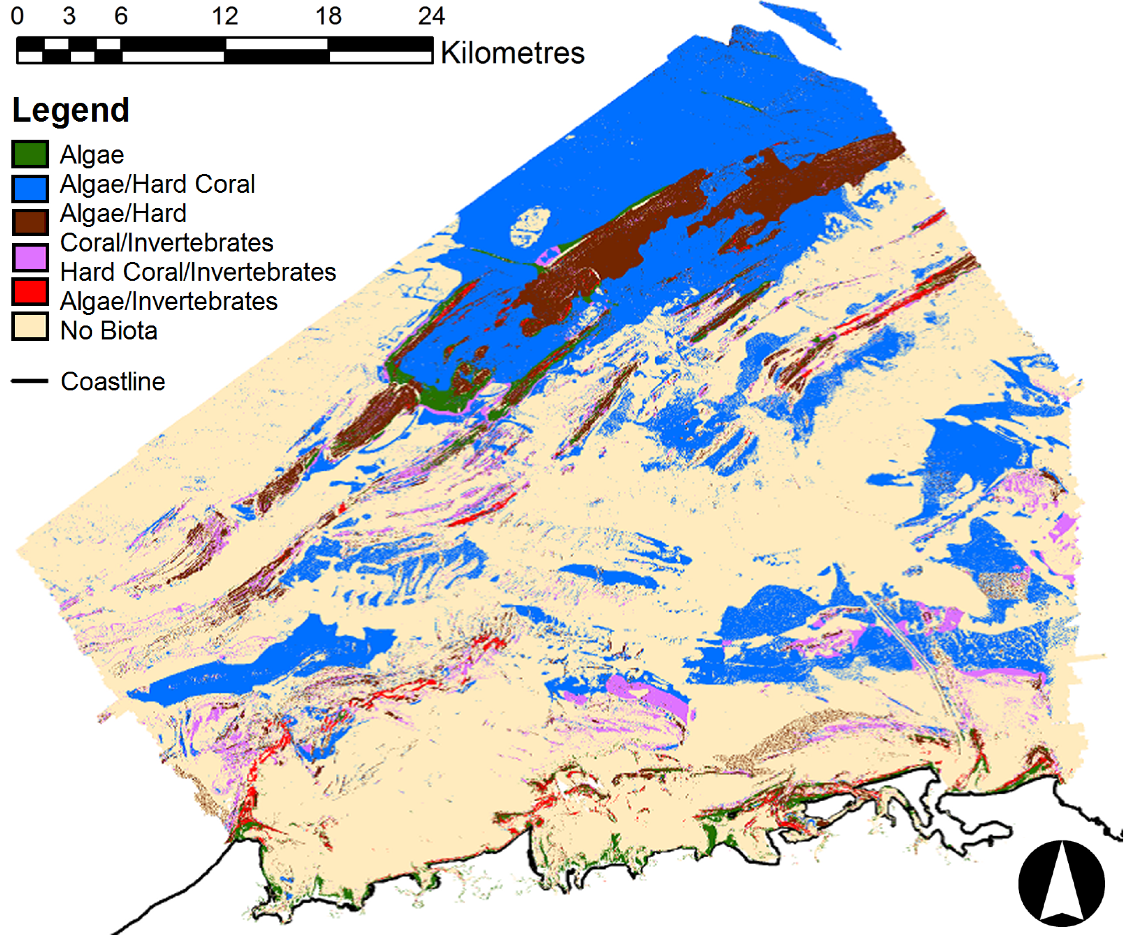
Figure 7 shows the final habitat classification map for the offshore Port Hedland region that has a spatial resolution of five metres. The classification results confirm that mixed habitat types are common. The largest class comprised “no epibenthos evident” (64.08%), which corresponded to mostly flat areas between major ridgelines. The largest habitat comprised areas of algae containing frequent hard corals. This habitat covered 23.47% of the mapped area, and was mostly found in the mid-shore regions and in the relatively flat offshore area in the north-east. Mixed environments, such as algae/hard corals/invertebrates (5.52%), and hard coral/invertebrates (3.58%) are the next most common groups, which occurred in association with mid-shore and offshore ridge lines. Only one class occurred that was comprised of a single biota type occurred (algae), which covered 1.76% of the area. Seagrass and Algae/Hard Coral were not classified due to lack of training data, inferring that they were very rare over the entire study region.

Figure 7. Final habitat classification result showing spatial distribution of habitats.

Figure 7. Final habitat classification result showing spatial distribution of habitats.

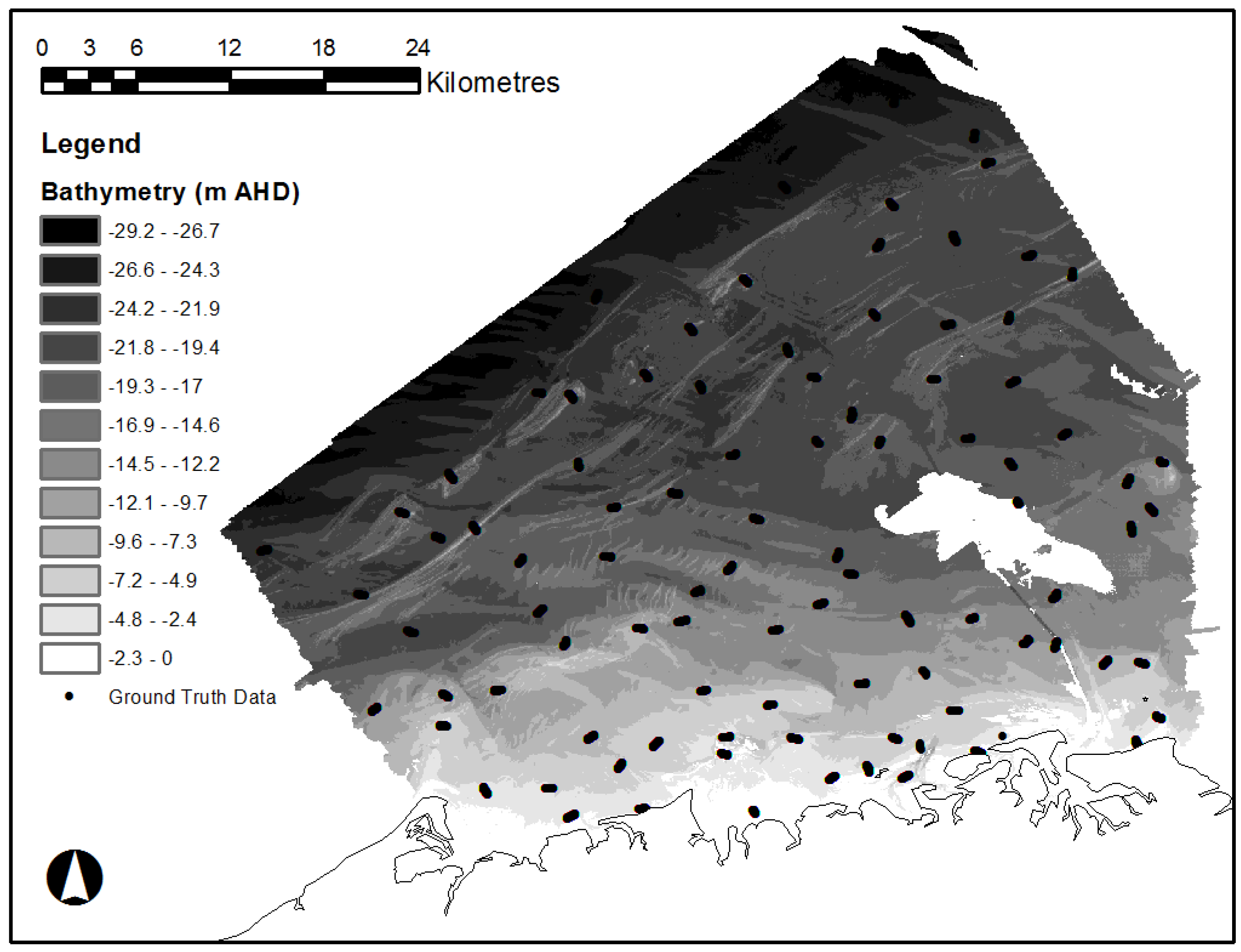
The “white” spaces in the LiDAR dataset represented a data gap captured during survey. Using the ground truthing data as a guide, this area was assumed to be entirely classified as “No Epibenthos Evident” (SKM, 2009) [26].

The relative aerial extent of each habitat class is provided in Table 4.

Table 4. Aerial extent of each significant habitat class identified in the mapping region as shown in Figure 7. * BPPH: Benthic Primary Producer Habitat. ** Sponge gardens and other non-photosynthetic invertebrates are not classed as BPPs, however their significance has been recognised in the Environmental Assessment Guideline 3 [24]. *** Excluding ephemeral benthic microalgae (and other photosynthetic biota) which should be considered BPPs, however are too small to detect in visual ground trothing program.

Classification	Type	Area (ha)	% of Survey Area
Algae	BPPH *	3629.28	1.76
Invertebrates	BPPH	48458.04	23.47
Algae/Invertebrates **	BPPH Mosaic	1831.55	0.89
Algae/Hard Coral/Invertebrates **	BPPH Mosaic	12863.25	5.52
Hard Coral/Invertebrates **	BPPH Mosaic	7390.21	3.58
No Epibenthos Evident	Non-BPPH (bare sediment) ***	132337.30	64.08
Total	N/A	206,509.62	100

Table 4. Aerial extent of each significant habitat class identified in the mapping region as shown in Figure 7. * BPPH: Benthic Primary Producer Habitat. ** Sponge gardens and other non-photosynthetic invertebrates are not classed as BPPs, however their significance has been recognised in the Environmental Assessment Guideline 3 [24]. *** Excluding ephemeral benthic microalgae (and other photosynthetic biota) which should be considered BPPs, however are too small to detect in visual ground trothing program.

Classification	Type	Area (ha)	% of Survey Area
Algae	BPPH *	3629.28	1.76
Invertebrates	BPPH	48458.04	23.47
Algae/Invertebrates **	BPPH Mosaic	1831.55	0.89
Algae/Hard Coral/Invertebrates **	BPPH Mosaic	12863.25	5.52
Hard Coral/Invertebrates **	BPPH Mosaic	7390.21	3.58
No Epibenthos Evident	Non-BPPH (bare sediment) ***	132337.30	64.08
Total	N/A	206,509.62	100

Analysis of Accuracy

An error matrix has been calculated for the final product (Table 5), based on the methodology outlined in the previous section titled “Error Assessment”. The overall accuracy (calculated as a percentage of accurate point predictions) of the six habitat classification has been found to be 97.6%, with a kappa coefficient of 0.9614. An error assessment for the classification that excluded the contributions of the hydrodynamic parameters gave a lower accuracy of 89.9% and kappa coefficient of 0.8372. This indicates an excellent classification result when hydrodynamic parameters are included with an improvement in accuracy of 7.7% (kappa increase of 0.1242) for this case study.

Table 5. Error matrix for the six habitat decision tree classification. Numbers in bold represent accurate incidences of classification.

Class	Algae	Invert	Algae/Invert	Algae/Hard Coral/Invert	Hard Coral/Invert	No Epibenthos Evident	Total
Algae	15	0	0	1	0	1	17
Invertebrates	0	179	0	0	0	1	180
Algae/Invert	1	0	37	3	0	1	42
Algae/Hard Coral/Invert	1	0	4	200	2	1	208
Hard Coral/Invert	0	0	0	0	58	4	62
No Epibenthos Evident	0	3	1	1	3	645	653
Total	17	182	42	205	63	653	1162

Table 5. Error matrix for the six habitat decision tree classification. Numbers in bold represent accurate incidences of classification.

Class	Algae	Invert	Algae/Invert	Algae/Hard Coral/Invert	Hard Coral/Invert	No Epibenthos Evident	Total
Algae	15	0	0	1	0	1	17
Invertebrates	0	179	0	0	0	1	180
Algae/Invert	1	0	37	3	0	1	42
Algae/Hard Coral/Invert	1	0	4	200	2	1	208
Hard Coral/Invert	0	0	0	0	58	4	62
No Epibenthos Evident	0	3	1	1	3	645	653
Total	17	182	42	205	63	653	1162

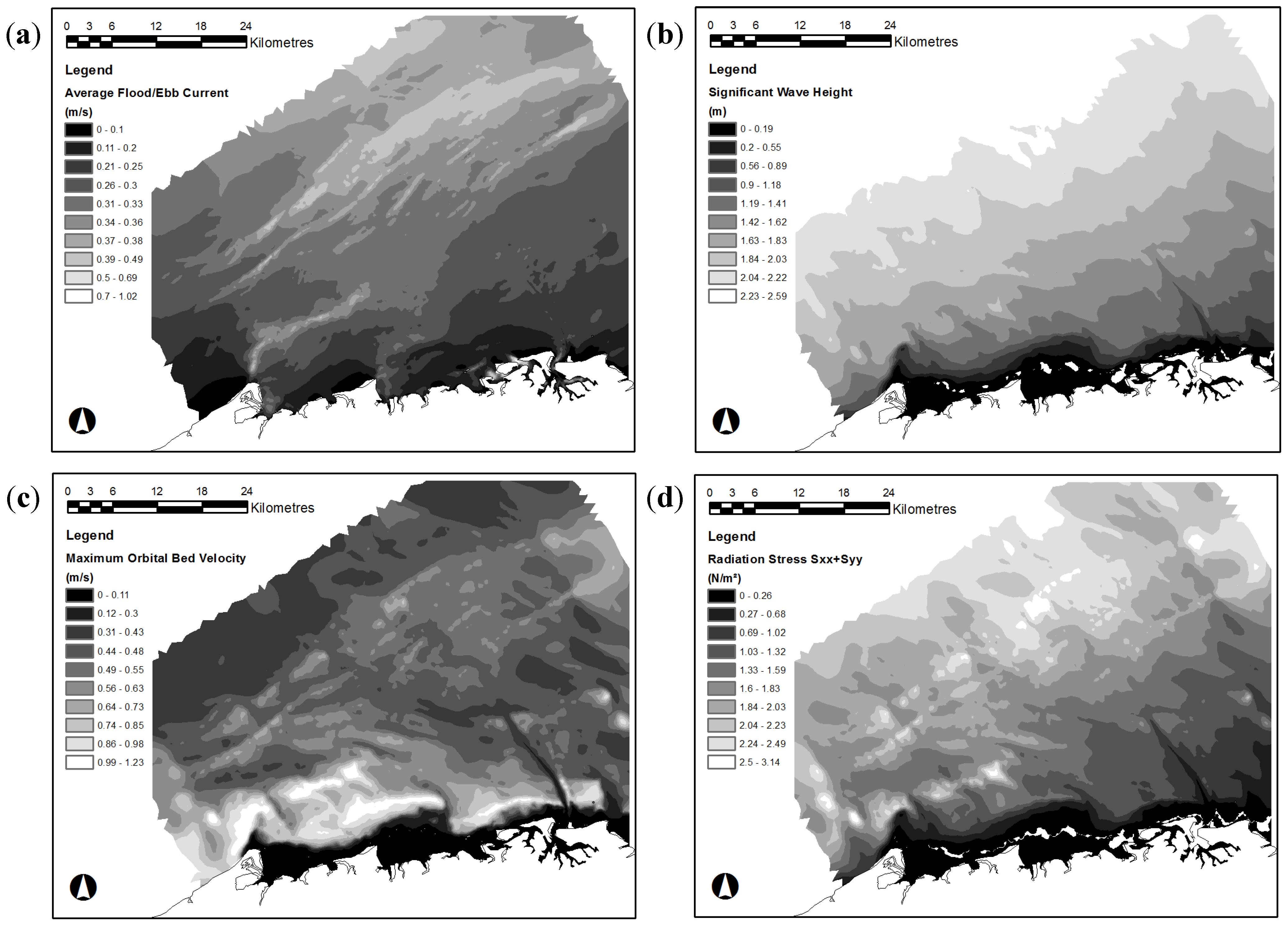
Further analysis was undertaken to determine the importance of each hydrodynamic parameter in the habitat mapping classification process at this particular location. This was achieved by removing each hydrodynamic parameter from the classification and documenting the corresponding accuracy achieved. Results from this exercise are shown in Table 6, and demonstrates that current was the least important hydrodynamic parameter, and the remaining three parameters related to wave action all contributed a similar amount to the classification accuracy. The best classification result was achieved by the inclusion of wave height, radiation stress, and orbital velocity, with the absence of current (although it was very similar to the accuracy that included all hydrodynamic parameters).

Table 6. Test results to determine importance of hydrodynamic parameters to the habitat mapping process.

Missing Hydrodynamic Data	Accuracy (%)	Kappa Coefficient
Significant Wave Height	94.6	0.9138
Current	97.9	0.9661
Radiation Stress	93.4	0.8948
Orbital Velocity	94.9	0.9199

Table 6. Test results to determine importance of hydrodynamic parameters to the habitat mapping process.

Missing Hydrodynamic Data	Accuracy (%)	Kappa Coefficient
Significant Wave Height	94.6	0.9138
Current	97.9	0.9661
Radiation Stress	93.4	0.8948
Orbital Velocity	94.9	0.9199

In the absence of “current” data, the accuracy and corresponding kappa coefficient is marginally higher than when all oceanographic parameters are included. This apparent inconsistency is explained in Langley and Iba [31], who demonstrated that when the number of input datasets increase for complex interactions, accuracy can decrease unless the number of training points also increases.

Overall, an area greater than 2000 km² was mapped during this study with a high level of accuracy (Kappa coefficient of >0.91). This is an excellent result particularly as traditional mapping methods heavily reliant on surveying would require many months of field time to produce a similar result, and would still require a large degree of interpolation (in the order of hundreds of metres [32]) over heterogeneous environments. Effective benthic habitat mapping over a large area can only be achieved when biological results are linked to broader scale surrogates in a meaningful way [1,2].

Issues with classification accuracy are often chiefly attributable to the inherent noise which occurs in the LiDAR bathymetry dataset, including noise issues such as turbidity and the misidentification of sediment dunes as reefs. However, this has not been a significant issue with this data, and with the incorporation of current and wave data, the confidence was predicated to increase from 89.9% to the present 97.6%. The opportunity to obtain and incorporate hydrodynamic parameters, which are a useful surrogate for benthic habitat type, adds significantly to the overall rigour of the predictive process [2,33].

As expected, the classification result was influenced by gaps in the LiDAR information which were addressed in post-processing to fill the gaps and form a complete dataset. Two of the habitat classes, seagrass and algae/hard coral, were extremely rare in the final classification map which was reflected in the survey data.

In previous automated habitat mapping projects in the Pilbara, a common issue has been misclassification of sediment dunes as rocky reef systems, as the macro-geomorphology of these features is largely similar. However, this issue was not significant in the current study, with dune features being classified as “No Epibenthos Evident”, separated by the “Invertebrate” class in deeper areas (as observed).

4. Conclusions

Hydrodynamic conditions can influence habitat types by directly impacting on marine organisms as well as having an influence on sediment transport and hence substrate type. Numerical modelling of hydrodynamics was used in this study as a method to take into consideration physical factors as an additional input into habitat classification, along with high resolution bathymetry and its associated geomorphic derivatives.

Spatially varying wave parameters were included into the decision tree algorithm to determine their relationship to the habitat classes at a location off the coast of Port Hedland. Classification accuracy was shown to improve from 89.9% to 97.9%, and a higher kappa coefficient increasing from 0.8372 to 0.9661. Habitat classes included in the classification were seagrass, algae, invertebrates, hard coral, and areas where there was no epibenthos evident.

The site selected for this investigation had a low presence of seagrass meadows, which are an important habitat in other coastal regions as they support highly productive and diverse ecosystems. Further work needs to be undertaken to determine the impact of hydrodynamics on seagrass to build on the important links that have been identified between them [14].

References

1. Diaz, R.J.; Solan, M.; Valente, R.M. A review of approaches for classifying benthic habitats and evaluating habitat quality. J. Environ. Manag. 2004, 73, 165–181. [Google Scholar] [CrossRef] [PubMed]
2. McArthur, M.A.; Brooke, B.P.; Przeslawski, R.; Ryan, D.A.; Lucieer, V.L.; Nichol, S.; McCallum, A.W.; Mellin, C.; Cresswell, I.D.; Radke, L.C. On the use of abiotic surrogates to describe marine benthic biodiversity. Estuar. Coast. Shelf Sci. 2010, 88, 21–32. [Google Scholar] [CrossRef]
3. Vierling, K.T.; Vierling, L.A.; Gould, W.A.; Martinuzzi, S.; Clawges, R.M. Lidar: Shedding new light on habitat characterization and modeling. Front. Ecol. Environ. 2008, 6, 90–98. [Google Scholar] [CrossRef]
4. Rattray, A.; Ierodiaconou, D.; Womersley, T. Wave exposure as a predictor of benthic habitat distribution on high energy temperate reefs. Front. Mar. Sci. 2015, 2, 1–14. [Google Scholar] [CrossRef]
5. Huang, Z.; Brooke, B.P.; Harris, P.T. A new approach to mapping marine benthic habitats using physical environmental data. Cont. Shelf Res. 2011, 31, S4–S16. [Google Scholar] [CrossRef]
6. Banic, J.; Cunningham, G. Airborne Laser Bathymetry: A tool for the Next Millennium; Optech Inc.: Toronto, Ontario, Canada, 1998; pp. 75–80. [Google Scholar]
7. Guenther, G.C. Airborne Laser Hydrography: System Design and Performance Factors; NOAA professional paper series, National Ocean Services 1; National Oceanic and Atmospheric Administration: Rockville, MD, USA.
8. Smith, R.A.; Irish, J.L.; Smith, M.Q. Airborne Lidar and airborne hyperspectral imagery: A fusion of two proven sensors for improved hydrographic surveying. In Proceedings of Canadian Hydrographic Conference, Montreal, Canada, 16–18 May 2000.
9. Guenther, G.C.; Cunningham, A.G.; Larocque, P.E.; Reid, D.J.; Service, N.O.; Highway, E.; Spring, S. Meeting the Accuracy Challenge in Airborne Lidar Bathymetry. In Proceedings of EARSeL-SIG-Workshop LIDAR, Dresden, FRG, 16–17 June 2000.
10. Finkl, C.W.; Benedet, L.; Andrews, J.L. Laser Airborne Depth Sounder (LADS): A New Bathymetric Survey Technique in the Service of Coastal Engineering, Environmental Studies, and Coastal Zone Management. In Proceedings of the 17th Annual National Conference on Beach Preservation Technology, Lake Buena Vista, FL, USA, 11–13 February 2004.
11. Eyre, B.D.; Maher, D. Mapping ecosystem processes and function across shallow seascapes. Cont. Shelf Res. 2011, 31, S162–S172. [Google Scholar] [CrossRef]
12. Ward, T.J.; Vanderklift, M.A.; Nicholls, A.O.; Kenchington, R.A. Selecting marine reserves using habitats and species assemblages as surrogates for biological diversity. Ecol. Appl. 1999, 9, 691–698. [Google Scholar] [CrossRef]
13. Hatcher, B.G.; Johannes, R.E.; Robertson, A.I. Review of research relevant to the conservation of shallow tropical marine ecosystems. Oceanogr. Mar. Biol. Annu. Rev. 1989, 27, 337–414. [Google Scholar]
14. Ryan, D.A.; Brooke, B.P.; Collins, L.B.; Spooner, M.I.; Siwabessy, P.J.W. Formation, morphology and preservation of high-energy carbonate lithofacies: Evolution of the cool-water Recherche Archipelago inner shelf, south-western Australia. Sediment. Geol. 2008, 207, 41–55. [Google Scholar] [CrossRef]
15. Ryan, D.A.; Brooke, B.P.; Collins, L.B.; Kendrick, G.A.; Baxter, K.J.; Bickers, A.N.; Siwabessy, P.J.W.; Pattiaratchi, C.B. The influence of geomorphology and sedimentary processes on shallow-water benthic habitat distribution: Esperance Bay, Western Australia. Estuar. Coast. Shelf Sci. 2007, 72, 379–386. [Google Scholar] [CrossRef]
16. Marrack, E.C. The Relationship Between Water Motion and Living Rhodolith Beds in the Southwestern Gulf of California, Mexico. Palaios 1999, 14, 159–171. [Google Scholar] [CrossRef]
17. Hills, D.J.; Jones, B. Peyssonnelid rhodoliths from the Late Pleistocene Ironshore Formation, Grand Cayman, British West Indies. Palaios 2000, 15, 212–224. [Google Scholar] [CrossRef]
18. Harris, P.T.; Baker, E.K. Geohab Atlas of Seafloor Geomorphic Features and Benthic Habitats: Synthesis and Lessons Learned. In Seafloor Geomorphology as Benthic Habitat; Elsevier: Amsterdam, The Netherlands, 2012; pp. 871–890. [Google Scholar]
19. Fugro LADS Mk 3 ALB System; Fugro Lads Corporation: Kidman Park, Australia, 2011; p. 2.
20. Cimmery, V. User Guide for SAGA (Version 2.0.5). Available online: http://www.saga-gis.org/en/about/references.html (accessed on 1 July 2012).
21. Sørensen, O.L.E.R.; Kofoed-Hansen, H.; Rugbjerg, M.; Sørensen, L.S. Using an Unstructured Finite Volume Technique. In Proceedings of the 29th International Conference on Coastal Engineering, Lisbon, Portugal, 19–24 September 2004.
22. Lumsden Point General Cargo Facility: Hydrodynamic Impact Assessment for EIA; WorleyParsons: Port Hedland, Western Australia, 2013; pp. 12–14.
23. Lumsden Point General Cargo Facility: Sediment Plume Dispersion Study for EIA; WorleyParsons: Port Hedland, Western Australia, 2013; p. 15.
24. EPA Environmental Assessment Guideline 3 (EAG3): Protection of Benthic Primary Producer Habitats in Western Australia’s Marine Environment; Event Personnel Australia: Perth, Australia, 2009; p. 41.
25. Mount, R.; Bricher, P.; Newton, J. National Intertidal/Subtidal Benthic Habitat Classification Scheme; National Land and Water Resources Audit: Hobart, Australia, 2007. [Google Scholar]
26. SKM Port Hedland Outer Harbour Development Marine Benthic Habitat Survey Report; SKM: Port Hedland, Australia, 2009; pp. 9–11.
27. Rattray, A.; Ierodiaconou, D.; Laurenson, L.; Burq, S.; Reston, M. Hydro-acoustic remote sensing of benthic biological communities on the shallow South East Australian continental shelf. Estuar. Coast. Shelf Sci. 2009, 84, 237–245. [Google Scholar] [CrossRef]
28. Foody, G.M. Status of land cover classification accuracy assessment. Remote Sens. Environ. 2002, 80, 185–201. [Google Scholar] [CrossRef]
29. Jensen, J.R. Introductory Digital Image Processing: A Remote Sensing Perspective, 3rd ed.; Prentice Hall: Upper Saddle River, NJ, USA, 2005; p. 526. [Google Scholar]
30. Mather, P.M. Computer Processing of Remotely Sensed Images, an Introduction; John Wiley & Songs Ltd: Chichester, West Sussex, UK, 2004; p. 324. [Google Scholar]
31. Langley, P.; Iba, W. Average-case analysis of a nearest neighbour algorithm. In Proceedings of the 13th International Joint Conference on Artificial Intelligence, Chambery, France, 28 August–3 September 1993; pp. 889–894.
32. Iocco, L.E.; Wilber, P.; Diaz, R.J.; Clarke, D.G.; Will, R.J. Benthic Habitats for New York/New Jersey Harbor: 1995 Survey of Jamaica, Upper, Newark, Bowrey, and Flushing Bays; NOAA Coastal Services Center: Silver Spring, MD, USA; US Army Corps of Engineers: Washington, DC, USA, 2000. [Google Scholar]
33. Mohn, C.; Beckmann, A. Numerical studies on flow amplification at an isolated shelfbreak bank, with application to Porcupine Bank. Cont. Shelf Res. 2002, 22, 1325–1338. [Google Scholar] [CrossRef]