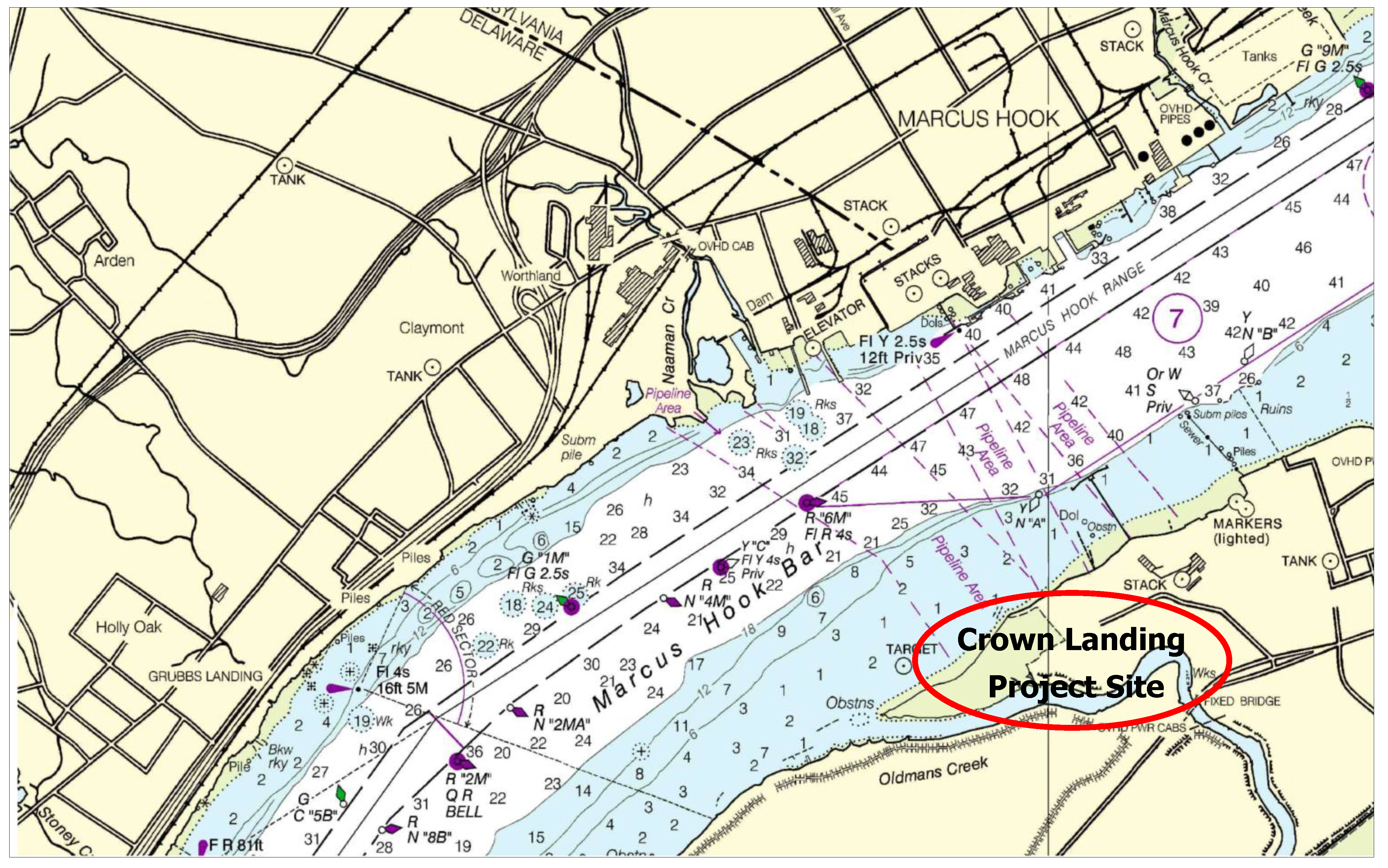
The case study used to demonstrate the entrainment computations and study the possible fish population-level impacts is vessel ballasting in an estuarine system. The site is located in the Delaware River Estuary where concerns were raised about the potential negative effects on the population of ichthyoplankton from entrainment during ballast water intake at the terminal berth and also the entrainment risk to sturgeon presented by the ballast intake. A 138,000 m
3 LNG carrier, the design vessel for this study, will withdraw approximately 8 million gallons [
11] of ballast water while at berth. The operations assume that one LNG carrier will call at the project every two to three days, resulting in approximately 150 ship calls per year or 12 per month. For the purposes of this study, the design intake rate of 660,430 gallons per hour and the design reballasting period of 12 h were selected.
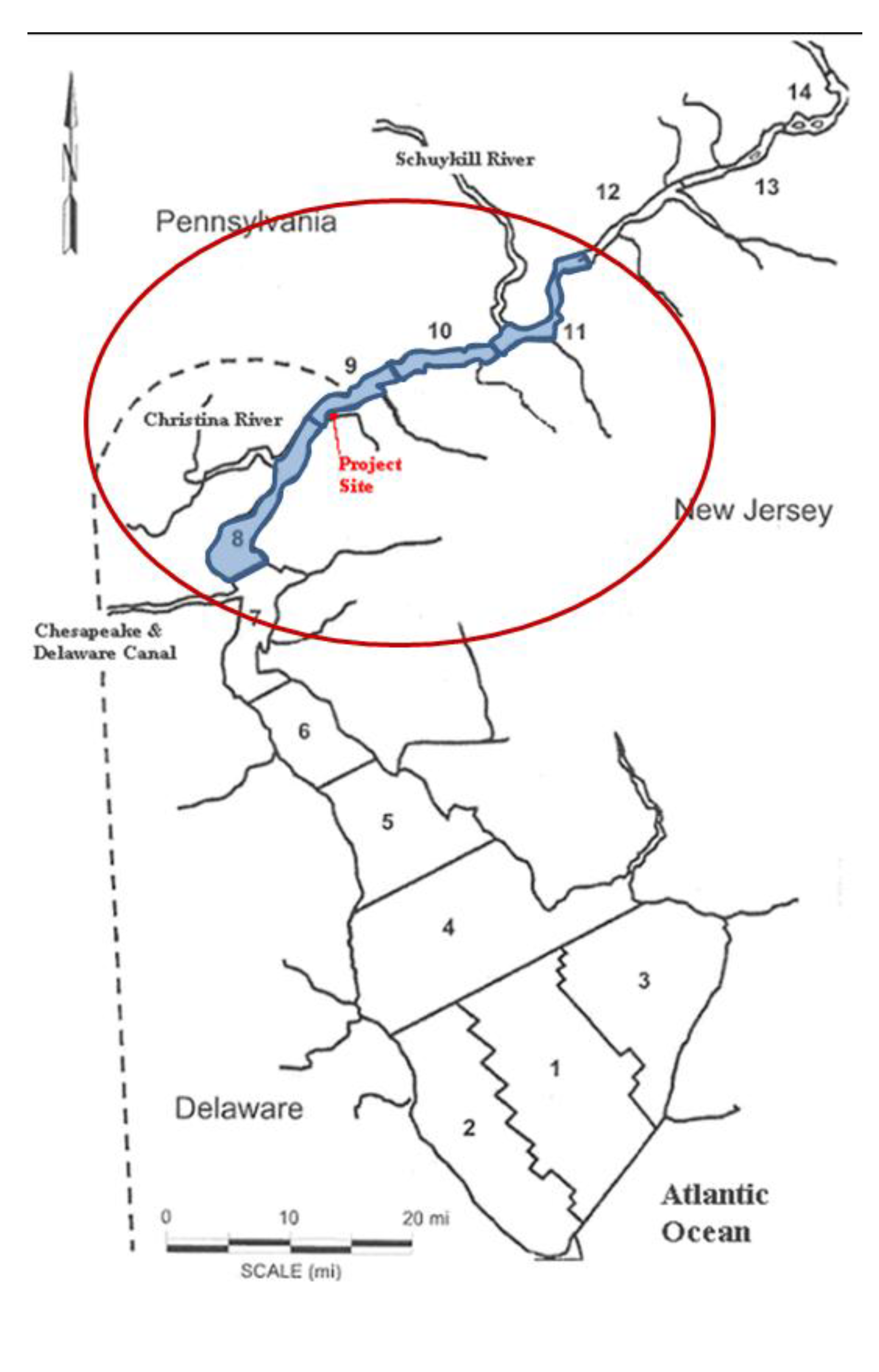
Figure 2 shows the site location in New Jersey near the state lines of Pennsylvania and Delaware.
4.1. Ichthyoplankton
Striped bass, white perch, clupeidae (river herring and American shad), and bay anchovy were the species and groups of concern since they consistently dominate the IP population in the project area. Mean IP densities between the months of April and July were available for the Delaware River in the project area. These density data were collected by PSEG during the springs of 2002 [
12] and 2003 [
13]. The density data were separated into different zones along the length of the Delaware River and, for purposes of this case study, it was assumed that these densities did not vary vertically and were composites of all trawls in each zone; however, the hydrodynamic model was divided into three vertical zones: epilimnion, metalimnion and hypolimnion. Only four zones (8–11) around the import terminal were considered as they covered a region of 25 miles downstream and 30 miles upstream (see
Figure 3). The entrainable population within these four zones is shown in
Table 1. IP is assumed to be present only during the months of April through July, so annual losses are calculated as a sum of these four months.
Figure 3.
Project location and IP data zones.
Figure 3.
Project location and IP data zones.
Table 1.
Entrainable IP by PSEG zone (number of organisms per 1000 ft3 of water).
Table 1.
Entrainable IP by PSEG zone (number of organisms per 1000 ft3 of water).
| Species/Group | Life Stage | Zone 8 | Zone 9 | Zone 10 | Zone 11 |
|---|
| Clupeidae (American Shad and River Herring) | Egg | 0.00 | 0.06 | 0.14 | 1.39 |
| Prolarvae | 0.00 | 0.51 | 1.64 | 8.92 |
| Postlarvae | 5.18 | 8.61 | 9.86 | 12.57 |
| Bay Anchovy | Egg | 0.00 | 0.00 | 0.00 | 0.00 |
| Prolarvae | 0.00 | 0.00 | 0.00 | 0.00 |
| Postlarvae | 72.13 | 0.57 | 0.03 | 0.00 |
| White Perch | Egg | 0.03 | 1.16 | 0.91 | 1.36 |
| Prolarvae | 0.65 | 0.76 | 1.19 | 3.34 |
| Postlarvae | 156.87 | 10.17 | 16.17 | 23.25 |
| Striped Bass | Egg | 31.44 | 41.4 | 1.05 | 0.54 |
| Prolarvae | 27.90 | 21.75 | 0.88 | 0.17 |
| Postlarvae | 938.00 | 5.8 | 7.1 | 0.86 |
Figure 4.
Ballast intake extent of influence.
Figure 4.
Ballast intake extent of influence.
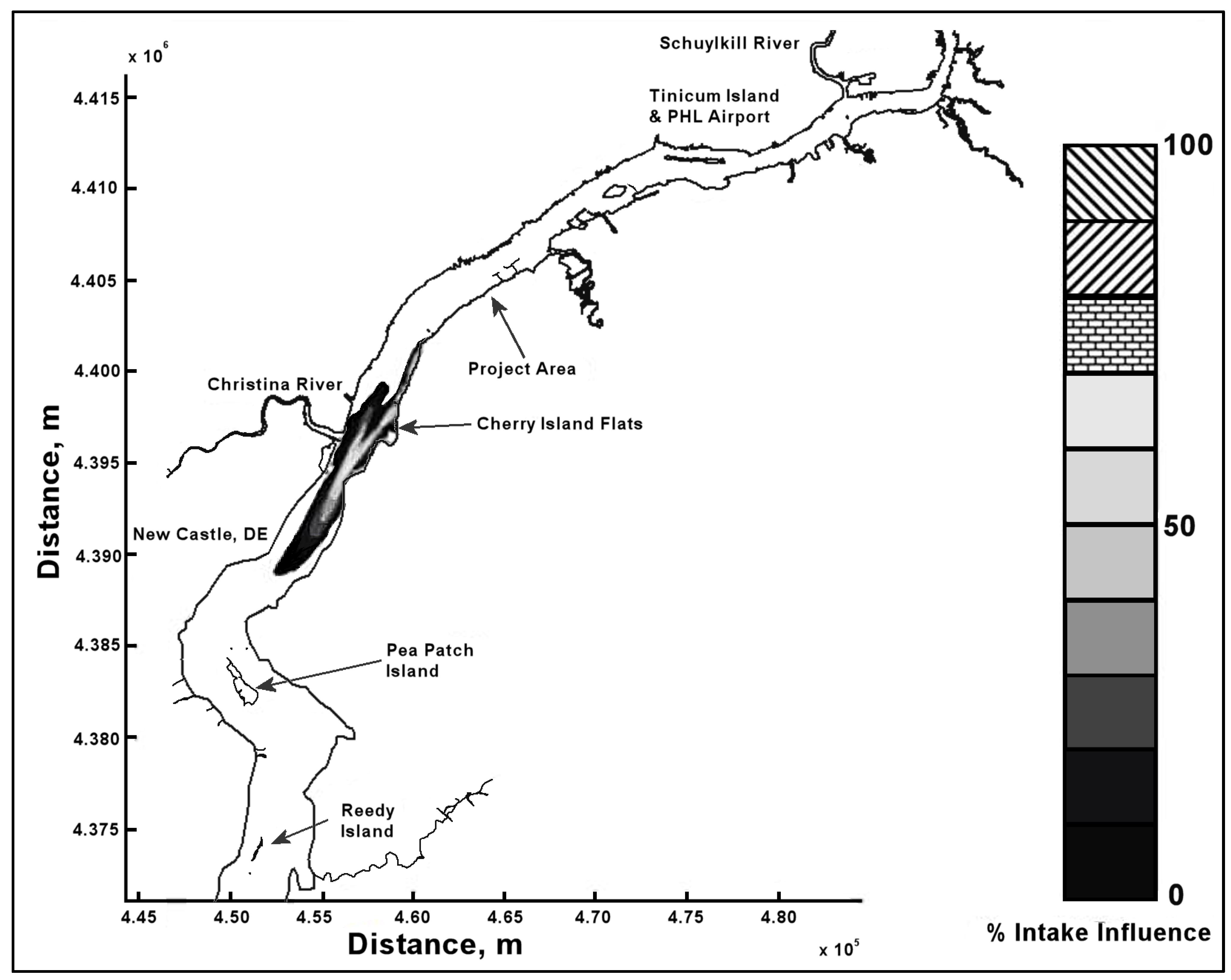
A hydrodynamic model and a water quality transport model were developed to evaluate the percentage of water entrained during a single ballast water intake at the project location. The numerical modeling protocol established in Edinger and Kolluru [
14] to estimate the entrainment of ichthyoplankton due to power plant cooling water intakes along a body of water was used as the basis for this study. Edinger and Kolluru divided the domain into several regions and used a numerical hydrodynamic model and a numerical transport model to simulate the entrainment of dye from each of these regions. The dye does not react or decay. The percentage of the dye entrained is used as a proxy to represent the amount of ichthyoplankton entrained. The model was based on the Delft3D [
1,
2] modeling system. The grid was created around the LNG terminal with grid sizes varying between 50 m and 200 m in the
x-direction (along the river) and 65 m and 100 m in the
y-direction (across the river). The grid extends all the way down to the Delaware Bay on the southern side and to Philadelphia on the northern side with 21,669 surface cells. The vertical resolution of the grid is chosen as 1 m. The model was run under flood and ebb conditions at the import terminal.
Figure 4 shows the extent of influence of the ballast intake as modeled.
The percentage of water entrained during each ballast water intake cycle during the flood condition is shown in
Table 2.
Table 2.
Percent of each water layer entrained by ballasting—flood condition.
Table 2.
Percent of each water layer entrained by ballasting—flood condition.
| Zone/Month | Percent Entrained from Epilimnion | Percent Entrained from Metalimnion | Percent Entrained from Hypolimnion |
|---|
| April |
| Zone 8 | 0.000% | 0.000% | 0.000% |
| Zone 9 | 0.033% | 0.012% | 0.017% |
| Zone 10 | 0.002% | 0.002% | 0.002% |
| Zone 11 | 0.000% | 0.000% | 0.000% |
| May |
| Zone 8 | 0.000% | 0.000% | 0.000% |
| Zone 9 | 0.034% | 0.012% | 0.018% |
| Zone 10 | 0.002% | 0.001% | 0.001% |
| Zone 11 | 0.000% | 0.000% | 0.000% |
| June |
| Zone 8 | 0.000% | 0.000% | 0.000% |
| Zone 9 | 0.034% | 0.012% | 0.017% |
| Zone 10 | 0.001% | 0.001% | 0.001% |
| Zone 11 | 0.000% | 0.000% | 0.000% |
| July |
| Zone 8 | 0.000% | 0.000% | 0.000% |
| Zone 9 | 0.035% | 0.012% | 0.017% |
| Zone 10 | 0.001% | 0.001% | 0.001% |
| Zone 11 | 0.000% | 0.000% | 0.000% |
These percentages were further used to estimate the entrainment potential for the four species based on their lifestage duration and natural mortality as shown in
Table 3 and
Table 4.
Table 3.
IP stage durations.
Table 3.
IP stage durations.
| Species/Group | Lifespan in Each Life Stage (Days) |
|---|
| Egg | Yolk Sac Larvae | Post-Yolk Sac Larvae |
|---|
| White Perch | 3 | 30 | 332 |
| Clupeidae | 6 | 53 | 306 |
| Striped Bass | 2 | 52 | 311 |
| Bay Anchovy | 1 | 34 | 330 |
Table 4.
Natural mortality rates.
Table 4.
Natural mortality rates.
| Species/Group | Natural Mortality in Each Life Stage (Day−1) |
|---|
| Egg | Yolk Sac Larvae | Post-Yolk Sac Larvae |
|---|
| White Perch | 0.601 | 0.164 | 0.005 |
| Clupeidae | 0.088 | 0.065 | 0.020 |
| Striped Bass | 0.601 | 0.164 | 0.005 |
| Bay Anchovy | 0.648 | 0.202 | 0.004 |
Overlaying the water capture fraction with the IP densities, life stage durations and natural mortality, the EAM model can calculate the effective entrainment. All four methods described previously were examined to compare the predictions of the different methods.
Table 5 summarizes the results and shows the predicted number of equivalent adults lost annually due to the intake operations. Methods 1 and 2 provide estimates of the likely upper and lower bound of the adults lost, while Methods 3 and 4 tend to give results reflective of the actual numbers likely to be lost.
Table 6 shows the equivalent number of adults lost as a percentage of total equivalent adults available within the entrainable zone. The projected number of adults lost are very small (maximum of 0.12%) and thus suggest that the intake operations will likely have very little effect on the regional fish populations, if any.
Table 5.
Total number of equivalent adults lost annually during flood and ebb condition ballast water intake operations using the four equivalent adult methods available in GEMSS-EAM.
Table 5.
Total number of equivalent adults lost annually during flood and ebb condition ballast water intake operations using the four equivalent adult methods available in GEMSS-EAM.
| Species/Group | Method 1 | Method 2 | Method 3 | Method 4 |
|---|
| Flood Condition |
| Clupeidae | 478 | 89 | 476 | 459 |
| Bay anchovy | 7472 | 1133 | 4245 | 2869 |
| White perch | 13,706 | 1325 | 9485 | 6618 |
| Striped bass | 30,671 | 5725 | 20,324 | 14,120 |
| Ebb Condition |
| Clupeidae | 360 | 55 | 357 | 344 |
| Bay anchovy | 16,425 | 994 | 9330 | 6270 |
| White perch | 15,454 | 1817 | 10,695 | 7473 |
| Striped bass | 110,427 | 3594 | 73,166 | 50,327 |
Table 6.
Total number of equivalent adults lost annually as percentage of total equivalent adults available in the entrainable zone (average of flood and ebb condition).
Table 6.
Total number of equivalent adults lost annually as percentage of total equivalent adults available in the entrainable zone (average of flood and ebb condition).
| Species/Group | Method 1 | Method 2 | Method 3 | Method 4 |
|---|
| Clupeidae | 0.01% | 0.00% | 0.01% | 0.01% |
| Bay anchovy | 0.00% | 0.00% | 0.00% | 0.00% |
| White perch | 0.00% | 0.00% | 0.00% | 0.00% |
| Striped bass | 0.12% | 0.02% | 0.08% | 0.05% |
The Methods 1 and 2 are clearly bounding approaches because Method 1 applies the entrainment mortality at the beginning of the life stage (largest population size within the life stage) whereas Method 2 applies entrainment mortality at the end of the life stage (smallest population size within the life stage). These two assumptions lead to Method 1 over predicting and Method 2 under predicting the actual losses. The remaining two models attempt to apply the entrainment mortality at a more reasonable point (within the life stage). Method 3 uses the midpoint of the life stage whereas Method 4 applies it continuously along with the entrainment mortality (net mortality which is a result of exponentially decaying population from entrainment and natural mortality individually). It is therefore important to bind the estimated impacts using these approaches along with considering the Method 4 as a more realistic estimate.
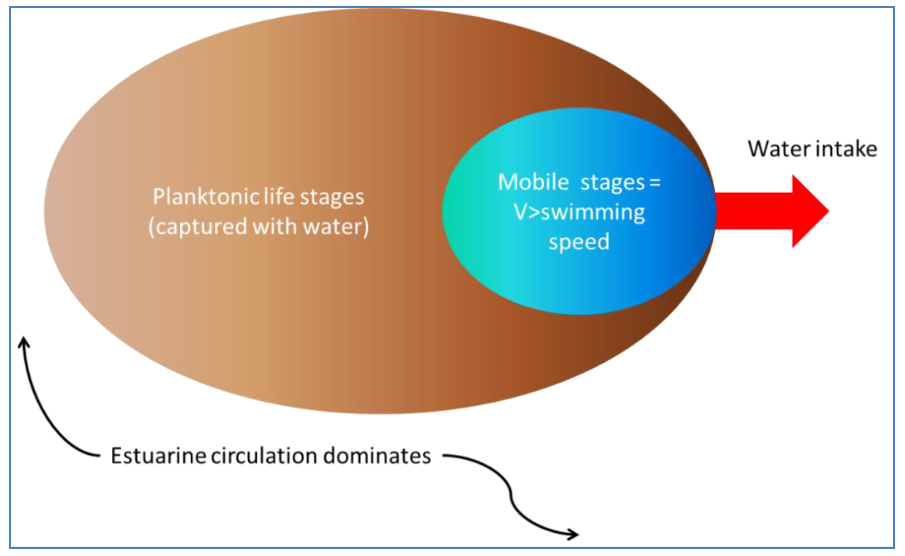
4.2. Zone of Influence—Sturgeon Effects
To address sturgeon entrainment, the zone of influence from the operation of the ballast water intake was studied using a second hydrodynamic model, GEMSS (Generalized Environmental Modeling System for Surface waters). A second model was applied to capture the level of detail required to evaluate the active swimming of fish as opposed to the passive entrainment of IP. The first step of the modeling was to create a high resolution near field grid around the ballast intake. The high resolution grid was created around this intake location with grid sizes varying between 10 m and 250 m in the
x-direction (along the river) and 15 m and 300 m in the
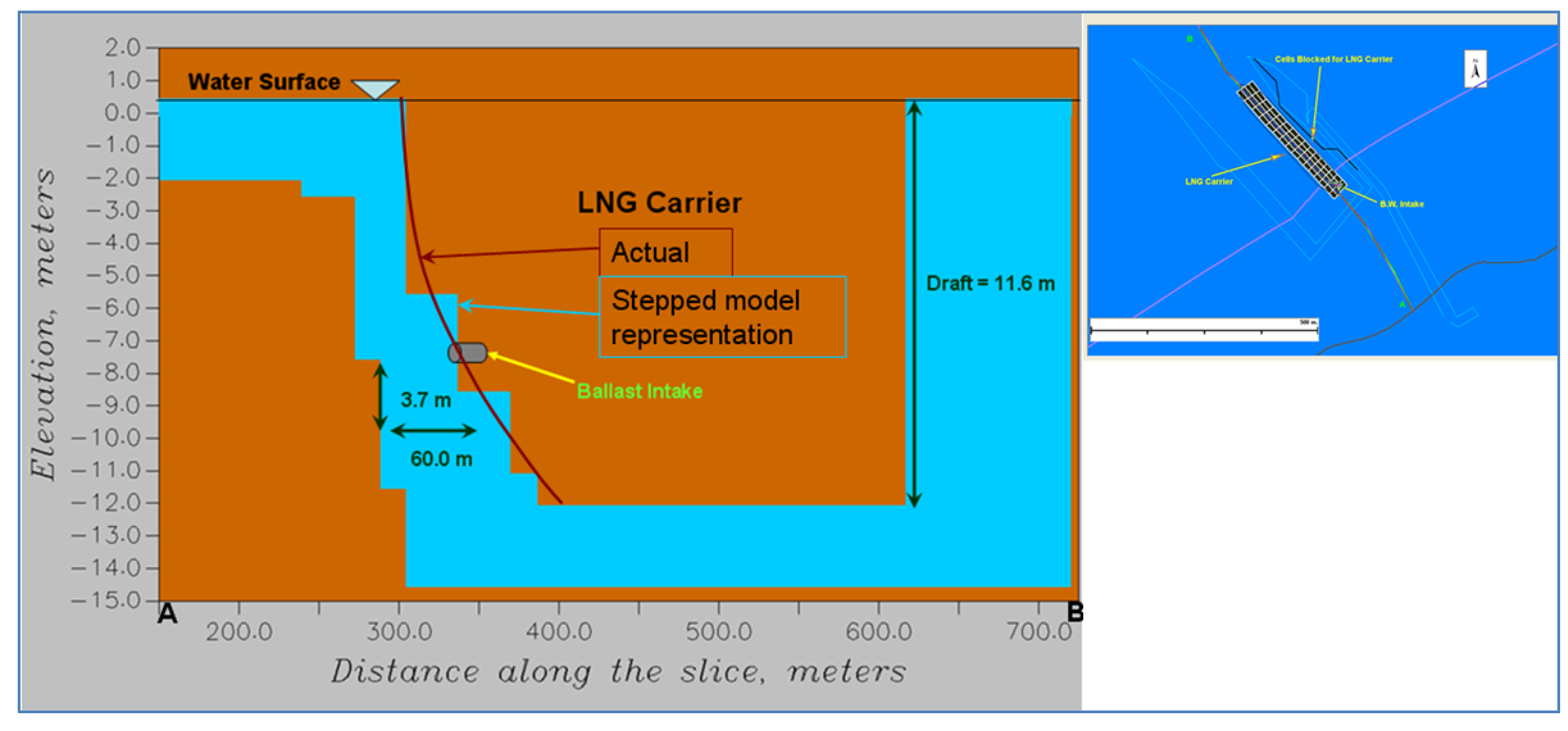
y-direction (across the river). The grid extends about 1 km on either side of the terminal along the river and covers the entire cross section with 1850 surface cells. The vertical resolution of the grid is chosen as 0.5 m. Based on the design information, the ballast intake of diameter 0.6 m (600 mm) and location of 3.7 m above the keel and 57 m forward of the stern was assumed. The high resolution model did not separate the two tidal cases as with the low resolution model earlier. The entire tidal cycle was combined into one model simulation to obtain cumulative effects. Some adults are long enough to become impinged if captured sidelong across the intake. Other mobile stages (adults and juveniles) can become entrained due to size or body orientation when they encounter the intake. These intake dimensions were closely followed in setting up the LNG carrier in the model domain as shown in
Figure 5.
Figure 5.
Carrier representation on the model domain.
Figure 5.
Carrier representation on the model domain.
Shortnose sturgeon have typical mean swimming speeds of 8.1 cm/s to 34.0 cm/s. These swimming speeds (and also burst speeds) are size dependent [
15]. McCleave [
16] found that the mean swimming speeds for shortnose sturgeon vary between 0.07 and 0.37 body lengths/s. Limited information is available about the swimming speeds for Atlantic sturgeon. Shortnose sturgeons are endangered species due the historical fishing and Atlantic sturgeon are similarly protected due to their resemblance to the shortnose. Entrainment of these sturgeons due to intake operations in the Delaware River is of concern. Sturgeons, and other species, as well can attain peak swimming speeds of up to 10–22 lengths/s [
15] under increased opposing flows. However, during these increased swimming speeds (burst speed), respiration increases which results in exhaustion decreasing the distance traveled. Thus, they are expected to escape high flow conditions if the zone of this high flow is less than their endurance. The swimming speeds for these sturgeons were obtained from Amaral and Sullivan [
17] and are summarized in
Table 7.
Table 7.
Swimming speeds.
Table 7.
Swimming speeds.
| Swimming/Speed Type | Sustained Duration | Speed | Fish Length |
|---|
| Maximum Sustained Speeds | >200 min | 4 cm/s | 15 cm |
| 84 cm/s | 120 cm |
| Prolonged Speeds | 20 s–200 min | 39 cm/s | 16 cm |
| 90 cm/s | 120 cm |
| 90 cm/s | 45 cm |
| Burst Speeds | <20 s | Same as Prolonged | Same as Prolonged |
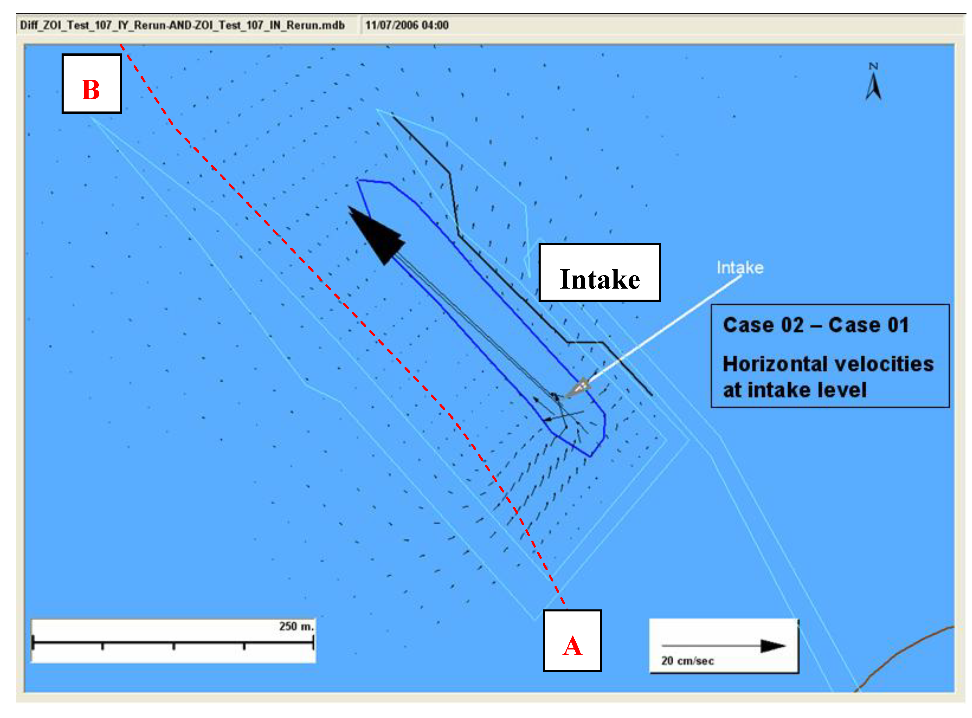
The ballast water intake was located at a depth as shown in
Figure 5. The high resolution model was run for two cases. Case 01 was run with the intake turned on whereas the Case 02 was run without the intake. These two cases were needed to determine the change in hydrodynamic conditions attributable to the intake operations. At this depth, in the near field, the horizontal velocity was predominantly towards the intake. There is a drastic difference in the horizontal velocities between the two cases. To better understand the effects due to the intake operation alone, consider
Figure 6, which shows the velocity difference (with intake—without intake). The difference was very high close to the intake (~35 cm/s) but this difference rapidly decreased with distance from the intake.
Figure 6.
Horizontal velocities at intake for each case.
Figure 6.
Horizontal velocities at intake for each case.
A northwest-southeast plane (Slice AB) passing through the ballast water intake, as shown in
Figure 5 and
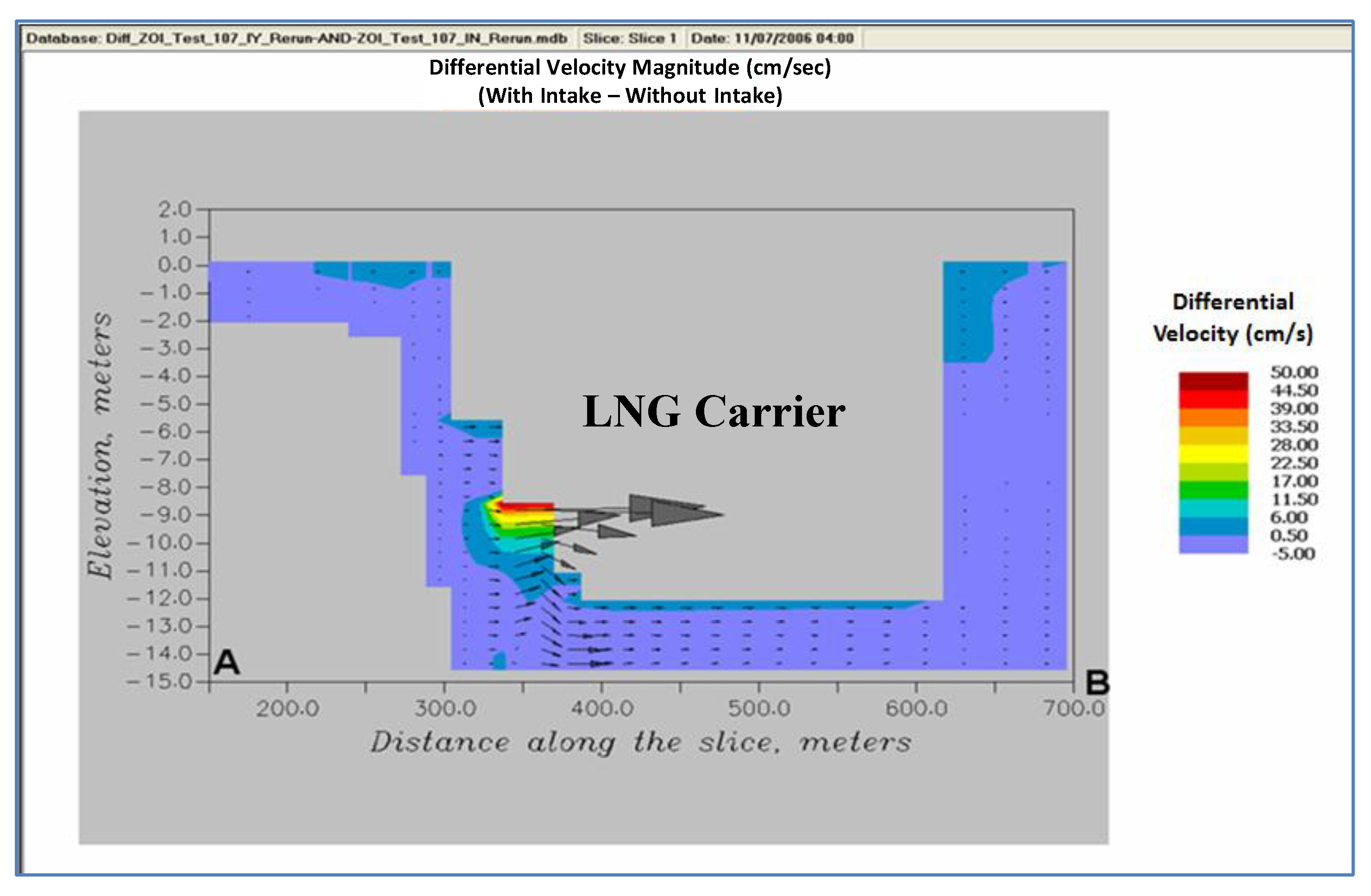
Figure 6, was chosen to study the vertical and northwest-southeast directional flow and zone of influence. The hydrodynamics of the region close to the intake is mostly dominated by the intake momentum as compared to the tidal influence. As we move slightly away from this region a small tidal variation in the circulation is seen under different tidal phases. The difference in the flow conditions between the two cases is shown in
Figure 7. The flows are high and directed towards the intake with a defined circulatory flow pattern. The effects of the intake, though smaller, can be seen even close to the bottom (~6 m below the intake). The difference in the velocity magnitude between the two cases is as high as 50 cm/s (
Figure 7). The differential velocity vectors clearly show a new eddy type circulation pattern introduced during the up estuary flow condition. The incremental velocity magnitude close to the bottom ranges between 0.5 cm/s and 6 cm/s. The zone of influence is about 5 m–6 m in the vertical direction and about 50 m in the horizontal direction. After around 50 m in the horizontal direction at the intake level, the difference in net velocity magnitude drops to 0.1% (<0.5 cm/s as compared to 50 cm/s at the intake cell).
Figure 7.
Differential velocities.
Figure 7.
Differential velocities.
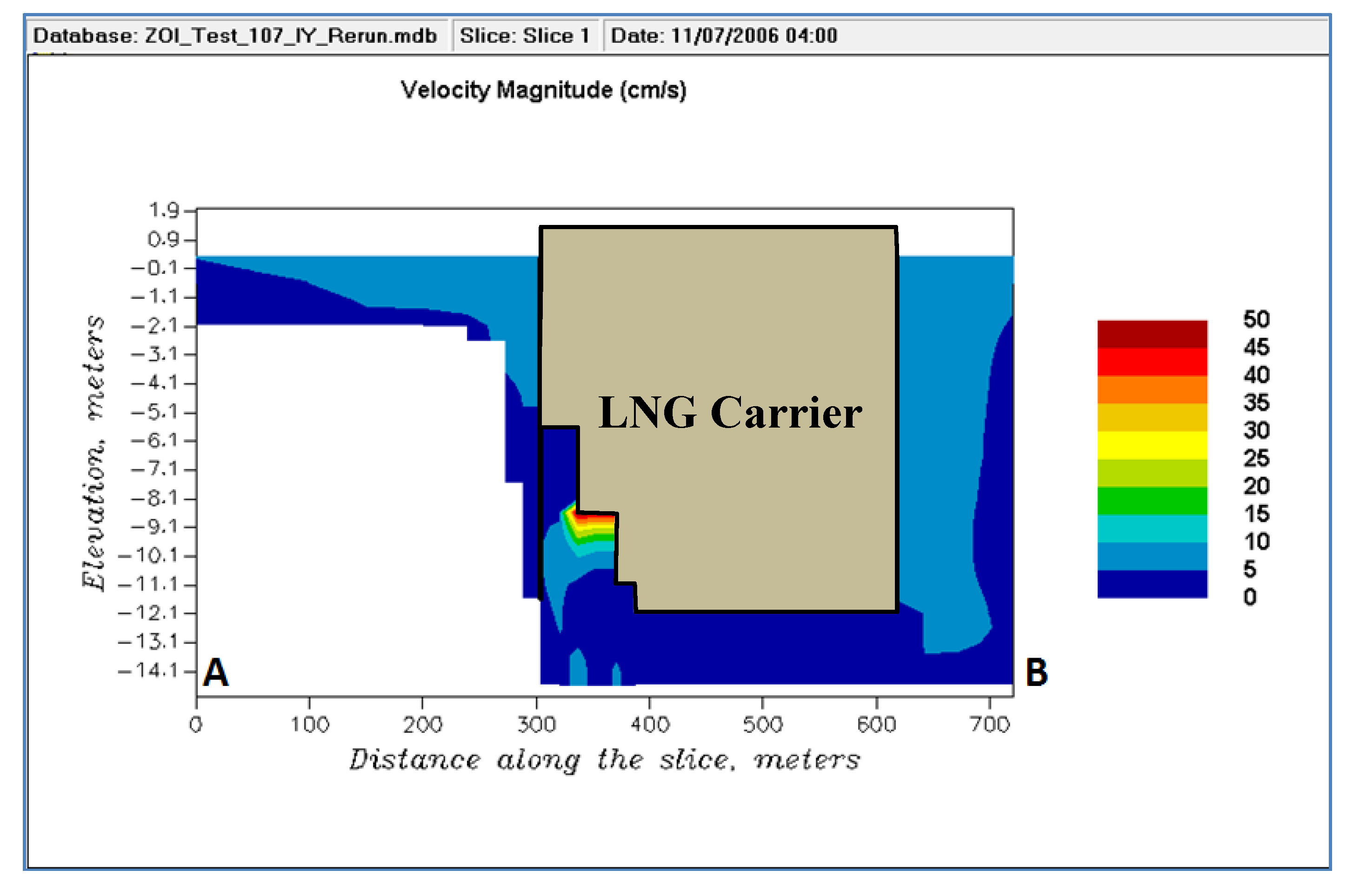
The mouth of the intake experiences the maximum increased flow (increase of 30–50 cm/s) which results in similar intake velocities of 30–50 cm/s (
Figure 8). These velocities at the intake when the ballast water intake is active are within the mean swimming speeds of both Atlantic and shortnose sturgeon. The burst speeds are much higher than the intake velocities and thus can allow them to escape the zone of influence. The burst swimming speeds cannot be sustained for a long duration (
Table 7). However, at these speeds (e.g., 90 cm/s) fish can move up to 18 m (90 cm/s × 20 s) to 54 m (90 cm/s × 60 s) which will move them out of the zone of influence (50 m). Even though the burst swimming speeds are not sustainable, the extent of the zone of influence is small to allow the fish to quickly escape. However, there may be instances when the fish are close to the intake and may be entrained due to the smaller net velocity (swimming speed—velocity towards intake). Only a volume of 13 m
3 was above the lowest burst swimming speed of 40 cm/s, a very small region.
Figure 8.
Velocity magnitude when intake is active.
Figure 8.
Velocity magnitude when intake is active.


