Article

Data Augmentation and Time–Frequency Joint Attention for Underwater Acoustic Communication Modulation Classification

Naval University of Engineering, Wuhan 430033, China
*
Author to whom correspondence should be addressed.
J. Mar. Sci. Eng. 2026, 14(2), 172; https://doi.org/10.3390/jmse14020172
Submission received: 19 November 2025 / Revised: 31 December 2025 / Accepted: 5 January 2026 / Published: 13 January 2026
(This article belongs to the Section Ocean Engineering)

Abstract

This paper presents a modulation signal classification and recognition algorithm based on data augmentation and time–frequency joint attention (DA-TFJA) for underwater acoustic (UWA) communication systems. UWA communication, as an important means of marine information transmission, plays a key role in fields such as marine engineering, military reconnaissance, and marine science research. Accurate recognition of modulated signals is a core technology for ensuring the reliability of UWA communication systems. Traditional classification and recognition methods, mostly based on pure neural network algorithms, suffer from insufficient feature representation and limited generalization performance in complex and changing UWA channel environments. They also struggle to address complex factors such as multipath, Doppler shift, and noise interference, often resulting in scarce effective training samples and inadequate classification accuracy. To overcome these limitations, the proposed DA-TFJA algorithm simulates the characteristics of real UWA channels through two novel data augmentation strategies: the adaptive time–frequency transform enhancement algorithm (ATFT) and dynamic path superposition enhancement algorithm (DPSE). An end-to-end recognition network is developed that integrates a multiscale time–frequency feature extractor (MTFE), two-layer long short-term memory (LSTM) temporal modeling, and a time–frequency joint attention mechanism (TFAM). This comprehensive architecture achieves high-precision recognition of six modulation types, including 2FSK, 4FSK, BPSK, QPSK, DSSS, and OFDM. Experimental results demonstrate that compared with existing advanced methods, DA-TFJA achieves a classification accuracy of 98.36% on the measured reservoir dataset, representing an improvement of 3.09 percentage points, which fully verifies the effectiveness and practical value of the proposed approach.

1. Introduction

The abundance of marine resources and the growing demand for their development and utilization have driven the rapid development of underwater acoustic (UWA) communication technology. In noncooperative UWA communication systems, the signal receiver often lacks relevant prior knowledge, which poses a challenge to signal recognition. Therefore, an effective noncooperative UWA communication signal modulation classification method is crucial for improving the real-time accuracy of signal recognition [1]. As advanced machine learning technology, neural networks can automatically learn and extract key features from signals. Their superior recognition ability and excellent environmental adaptability have been widely used in modulation classification tasks [2]. However, the training of neural network models usually relies on much labeled data and can be used only for real-time signal classification after training is completed. This data-driven learning mechanism places high demands on the quantity and quality of training samples. If the actual collected signal data are limited in scale, the model is prone to a decrease in classification accuracy because insufficient training severely affects the overall performance of the algorithm [3]. As an effective means of data expansion and perturbation, data augmentation technology generates rich sample data through a variety of algorithms to address the insufficient dataset size [4,5]. This technique was first popularized in computer vision. Common enhancement operations include image flipping, scaling, rotation, and cropping [6]. These methods have been proven to significantly improve the training effect of the model [7]. As research has progressed, scholars have proposed a variety of combinations and improved methods for enhancement strategies. AugMix [8] and RandAugment [9] improve the robustness of the model through multiple or simplified random enhancement combinations; Cutout [10] and Random Erasing [11] use image occlusion mechanisms to enhance the model’s ability to perceive context; and the generative adversarial network (GAN) has also been introduced into data augmentation tasks to further expand the ideas and boundaries of enhancement technology by generating realistic samples [12,13].
With the increase in the demand for robust, generalized and small-sample recognition in automatic modulation classification (AMC) in complex channels, low signal-to-noise ratios (SNR) and cross-scenario applications, data augmentation methods are being applied to modulation signal recognition. One type of method uses image representation to convert modulation signals into constellation diagrams, spectrum diagrams, etc., and applies enhancement methods in the visual field in the form of image recognition. As shown in Table 1, the related works are summarized as follows. Y. Peng et al. [14] simulated the signal phase shift by rotating the signal constellation diagram by a specific angle, thereby enhancing the robustness of the model to phase changes. However, insufficient constellation diagram data still exist. To solve the data scarcity problem, L. Yin et al. [15] used a GAN to generate synthetic constellations for training data expansion, effectively improving the generalization ability of the model. Another type of method directly designs data augmentation strategies for the original signal that are more suitable for the original domain learning process of building lightweight models. N. Wang et al. [16] expanded the sample space by signal rotation and designed a RandMix strategy that fused multiple data enhancements, providing a powerful and novel solution to the domain shift problem in AMC. However, its computational complexity is too high for it to be applied in practical environments. To solve this problem, A. Gong et al. [17] fused I/Q and A/P representations and introduced rotation and self-perturbation mechanisms to improve recognition performance, effectively improving the adaptability of the model to complex environments. This data augmentation method improves the recognition rate of most signals, but the recognition rate of certain specific modulation types is limited. To address the above problems, W. Shen et al. [18] proposed a data augmentation framework based on mixed signals. By mixing signal samples of the same modulation type, new training samples are generated, thereby expanding the dataset and improving model performance, effectively improving the modulation classification accuracy. However, this method destroys the temporal dependency of the signal, causing unnecessary noise to be introduced into the data or causing the network model to learn incorrect data. To improve the authenticity of the signal generated by data augmentation, M. Li et al. [19] used a conditional diffusion model to generate high-fidelity and diverse signal samples, effectively solving the problem concerning the insufficient training data in AMC tasks. The underwater environment differs from the conventional communication environment. Conventional data augmentation methods cannot generate new training samples that meet the characteristics of UWA communication for UWA communication signal data, and the effect on improving model performance is not good. Further research is needed. While the aforementioned methods have made some progress in modulated signal classification, they still face challenges such as insufficient coupling between enhancement strategies and UWA propagation mechanisms, inadequate characterization of complex channel disturbances such as multipath and time-varying Doppler effects, and insufficient representation capabilities of feature extraction networks in complex environments. To address the scarce training samples and insufficient classification accuracy in complex channel environments in UWA communication signal recognition, we propose a modulated signal classification and recognition algorithm based on data augmentation and time–frequency joint attention (DA-TFJA).
(1) For data augmentation, this work designs two algorithms: the adaptive time–frequency transform enhancement algorithm (ATFT) and the dynamic path superposition enhancement algorithm (DPSE) that simulate the characteristics of realistic UWA channels from the perspectives of time–frequency-domain variations and multipath propagation, respectively.
(2) For network architecture, this work constructs an end-to-end recognition network integrating a multi-scale time–frequency feature extraction module (MTFE), two-layer long short-term memory (LSTM) temporal modeling, and a time–frequency joint attention mechanism (TFAM). This network processes multi-scale time–frequency features, captures long-term temporal dependencies, and adaptively focuses on key information, thereby achieving feature extraction for UWA communication signals.
(3) Experimental results demonstrate that the proposed algorithm achieves a classification accuracy of 98.36% on a measured dataset. The algorithm maintains excellent performance under low SNR and long-distance transmission conditions, achieving an accuracy of 65.21% at an SNR of −4 dB, fully demonstrating the algorithm’s practical value.

2. DA-TFJA

2.1. Algorithm Framework

DA-TFJA achieves high-precision recognition of modulated signals in complex UWA environments by integrating multilevel feature extraction and an intelligent attention mechanism. The original UWA communication signal is processed using two parallel data augmentation branches: one branch is subjected to the ATFT algorithm, which simulates the time-varying characteristics of the UWA channel through a time-domain Doppler transform and frequency-domain carrier offset; the other branch is subjected to the DPSE, which simulates a realistic multipath propagation environment through multipath parameter generation and signal superposition. The enhanced signal data, along with the original signal, are input into the MTFE. The MTFE employs a four-branch parallel convolutional architecture, using convolution kernels of four different sizes—1 × 3, 1 × 5, 1 × 7, and 3 × 1—to capture short-term, medium-term, long-term, and frequency-domain features, respectively. The spatial features extracted by the MTFE are flattened and then fed into an LSTM network for time series modeling. Each LSTM layer contains 128 units, and the LSTM network outputs a high-dimensional feature representation rich in temporal information. The temporal features output by the LSTM network are fed into the TFAM for attention enhancement. The TFAM first reorganizes the features into a two-dimensional time–frequency representation. It then calculates time-domain attention, frequency-domain attention, and time–frequency cross-attention separately, generating a comprehensive attention weight through an adaptive fusion strategy. This mechanism automatically identifies time periods and frequency components containing key modulation information, suppresses the effects of noise and multipath interference, and outputs discriminative features enhanced with attention. These enhanced features are then fed into a classifier for final modulation type identification, outputting classification probabilities for six modulation types: 2FSK, 4FSK, BPSK, QPSK, DSSS, and OFDM. The overall algorithm design is shown in the Figure 1 below.

2.2. Data Augmentation Algorithm

2.2.1. ATFT

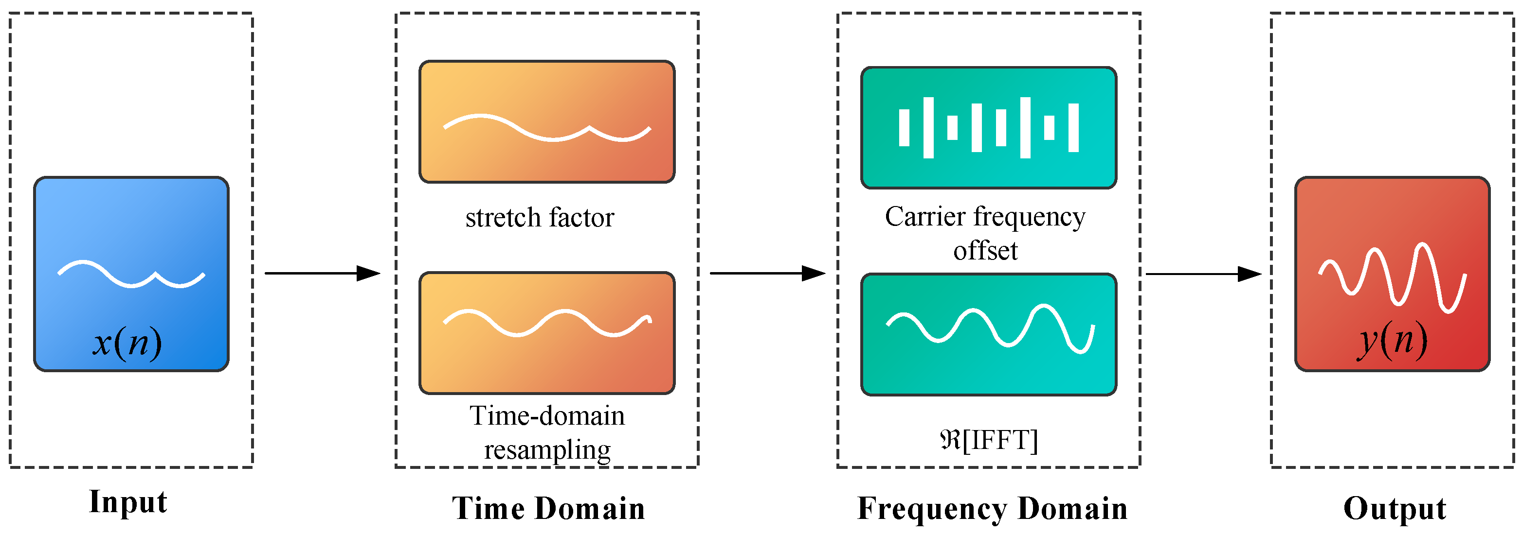
In UWA communication signal recognition, the complexity of the real underwater environment and the limited data acquisition costs often result in a limited number of available training samples that severely impact the generalization and classification accuracy of deep learning models. UWA channels exhibit complex characteristics, such as time variations, multipath effects, and Doppler shifts, resulting in significant differences in signals collected at different times and under different environmental conditions. To increase the model’s robustness to these channel variations and improve the reliability of recognition algorithms in practical applications, data augmentation techniques are necessary to increase the number and diversity of training samples [20]. We propose an ATFT that simulates the key physical properties of UWA channels to generate enhanced samples that exhibit realistic channel effects. As shown in the Figure 2 below, the steps of ATFT are as follows:
1. Assume that the original received signal is x ( n ) , n = 0 , 1 , , N 1 , where N is the duration. The original UWA communication signal is input, and basic amplitude normalization processing is performed to eliminate the differences in amplitude between different samples caused by factors such as propagation distance and transmission power, providing a unified benchmark for subsequent transformations. The mathematical expression is as follows:
x 0 ( n ) = x ( n ) max | x ( n ) |
2. On the basis of the possible relative motion between the transmitter and receiver in the UWA environment, a Doppler effect stretch factor is randomly generated for subsequent time-domain transformation operations. The mathematical expression is as follows:
α = 1 + δ
where δ U ( 0.03 , 0.03 ) is a uniformly distributed random Doppler coefficient.
3. The generated Doppler parameters are used to resample the signal in the time domain to simulate the Doppler effect caused by the relative motion between the transmitter and the receiver, which changes the time scale of the signal. The mathematical expression is as follows:
x 1 ( n ) = x 0 n α
where n is the discrete time index of the current signal and x 1 ( n ) is the output signal after the time-domain stretching/compression transformation. Since the obtained x 1 ( n ) is usually a noninteger, linear interpolation is used for representation:
x 1 ( n ) = x 0 ( m ) + x 0 ( m + 1 ) x 0 ( m ) · ( t m )
where t = n α , m = t , and t represents the time t rounded down.
4. After time-domain transformation, the signal is converted to the frequency domain, and the carrier frequency offset is applied to simulate the carrier frequency drift caused by factors such as clock asynchrony between the transmitter and receiver and the time-varying characteristics of the channel. The time-domain signal x 1 ( n ) from step 3 is converted to the frequency domain using the Discrete Fourier Transform (DFT), yielding the frequency-domain representation X ( k ) , where k is the discrete frequency bin index (k = 0, 1,..., N − 1). The DFT transformation is expressed as:
X ( k ) = n = 0 N 1 x 1 ( n ) · e j 2 π k n N
The mathematical expression of the carrier frequency offset is as follows:
X 1 ( k ) = X ( k ) · e j 2 π ε k
where ε U ( 0.015 , 0.015 ) is the normalized carrier frequency offset coefficient.
5. The signal processed by the frequency-domain carrier frequency offset (CFO) is transformed back to the time domain to obtain a time-domain signal that includes both the Doppler effect and the CFO effect. The mathematical expression is as follows:
x 2 ( n ) = 1 N k = 0 N 1 X 1 ( k ) · e j 2 π k n N
Here, [ · ] represents the real part operator, which ensures that the output is a real-valued signal.
6. Amplitude restoration is performed on the transformed signal to ensure that the enhanced signal has the same energy level as the original signal has and maintain the power characteristics and signal-to-noise ratio of the signal. The mathematical expression is as follows:
x out ( n ) = x 2 ( n ) · A ref A cur
where A r e f = 1 N n = 0 N 1 x 0 2 ( n ) is the RMS value of the original signal and A c u r = 1 N n = 0 N 1 x 2 2 ( n ) is the RMS value of the current signal.
7. Through the above steps, the final output of the adaptive time–frequency transform enhancement algorithm is as follows:
y ( n ) = x out ( n ) , n = 0 , 1 , , N 1

2.2.2. DPSE

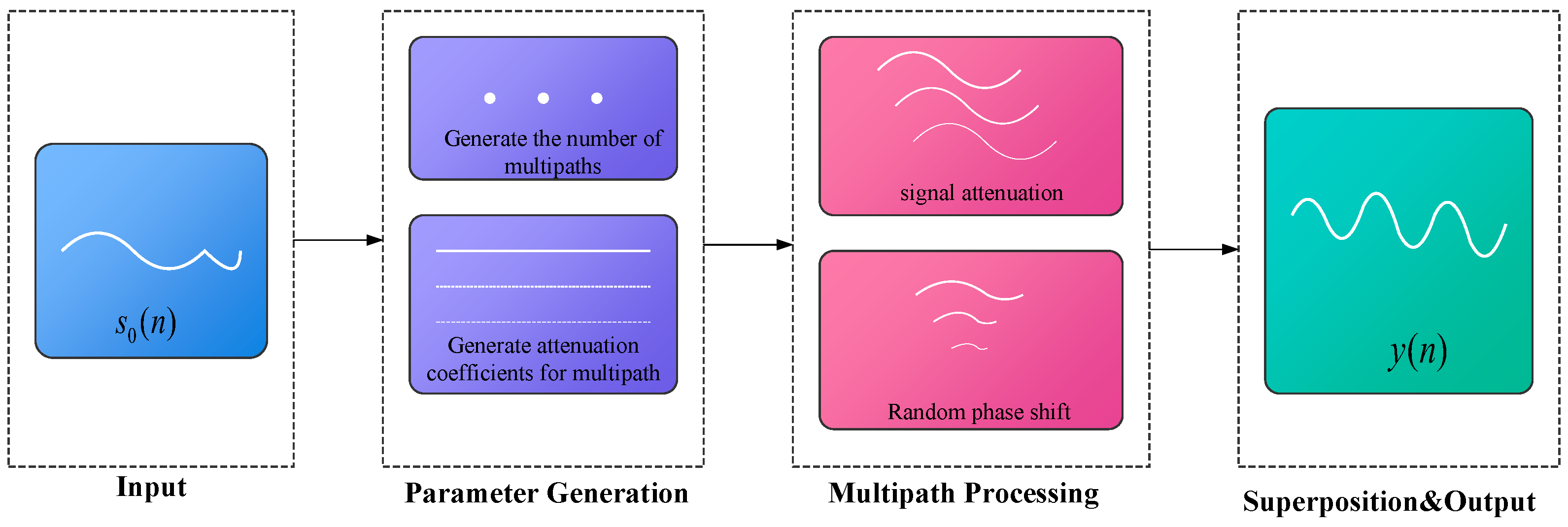
In UWA communication signal recognition tasks, multipath propagation in the actual ocean environment is among the main factors affecting signal quality and classification accuracy. Because of reflection and refraction at interfaces such as the seabed, sea surface, and thermocline, the receiver often receives multiple copies of the signal propagated through different paths, each with different delay, attenuation, and phase characteristics. Traditional datasets often lack samples of such complex multipath environments, resulting in the poor performance of trained models in complex channel environments. To improve the robustness of the model to multipath interference and classification accuracy in real UWA environments, data augmentation techniques are needed to simulate various possible multipath propagation scenarios [21]. We propose the DPSE, which simulates the multipath effects of real UWA channels by superimposing multiple propagation paths with different delay and attenuation characteristics on the original signal.
As shown in the Figure 3 below, the steps of the DPSE are as follows:
1. Amplitude normalization is performed on the input raw UWA communication signal to ensure consistency across different samples. The mathematical expression is as follows:
s 0 ( n ) = x ( n ) 1 N n = 0 N 1 x 2 ( n )
where x ( n ) is the original received signal and N is the duration.
2. On the basis of the statistical characteristics of the UWA environment, key parameters of multipath propagation, including the number of multipaths, delay time, and attenuation coefficient, are randomly generated to simulate the random variation characteristics of multipath parameters in the actual ocean environment. The multipath number is expressed as follows:
L = randint 1 , L max
where L is the randomly generated multipath number, which ranges from 1 to L max (usually set to 3). The delay time is expressed as follows:
τ l = uniform 0.5 × 10 3 , τ max , l = 1 , 2 , , L
where τ l is the delay time of the lth multipath, which is uniformly distributed between 0.5 ms and τ max (usually 5 ms). The attenuation coefficient is expressed as follows:
β l = uniform ( 0.1 , 0.5 ) × e τ l τ c , l = 1 , 2 , , L
where β l is the attenuation coefficient of the lth multipath. The basic attenuation is uniformly distributed between 0.1 and 0.5, multiplied by the exponential attenuation factor e τ l τ c (where τ c is the attenuation time constant).
3. On the basis of the generated multipath parameters, the original signal is delayed to generate delayed signal copies corresponding to different propagation paths. The mathematical expression is as follows:
d l = round τ l × f s
s l ( n ) = 0 n < d l s 0 n d l n d l
where d l is the number of delayed sampling points corresponding to the lth multipath, round(.) represents rounding, and s l ( n ) is the delayed signal of the lth multipath. The first d l sampling points are 0 (indicating that the signal has not yet arrived), and starting from the d l th sampling point, it is a delayed copy of the original signal.
4. The corresponding attenuation and phase-induced amplitude variation are applied to each multipath signal to simulate the energy loss and interference effects on different propagation paths. The mathematical expression is as follows:
ϕ l = uniform ( π , π )
s l ( n ) = β l × s l ( n ) × cos ϕ l
where ϕ l is the random phase of the lth multipath uniformly distributed within [ π , π ] . The term cos ( ϕ l ) represents the amplitude variation caused by phase differences between multipaths, simulating constructive and destructive interference effects when signals from different paths are superimposed at the receiver. s l ( n ) represents the lth multipath signal after attenuation and phase processing, β l represents the previously generated attenuation coefficient.
5. The original signal and all the processed multipath signals are linearly superimposed to form a composite signal that includes the multipath effect. The mathematical expression is as follows:
s multipath ( n ) = s 0 ( n ) + l = 1 L s l ( n )
where s multipath ( n ) is the composite signal after multipath superposition, which is composed of the linear superposition of the original direct signal s 0 ( n ) and all multipath components s l ( n ) . The summation term l = 1 L s l ( n ) represents the sum of all L multipath signals.
6. Power normalization is performed on the superimposed multipath signals to ensure that the output signal has the same energy level as the original signal has and to maintain the consistency of the dataset. The mathematical expression is as follows:
P ref = 1 N n = 0 N 1 s 0 2 ( n )
P current = 1 N n = 0 N 1 s multipath 2 ( n )
y ( n ) = s multipath ( n ) × P ref P current
where P ref is the average power of the original signal and P current is the average power of the multipath superposition signal. By multiplying the power adjustment factor P ref P current , the power of the output signal y ( n ) is kept consistent with that of the original signal.
Using the ATFT and DPSE data augmentation algorithms, the original UWA communication dataset is significantly expanded and enriched, with the training set size increasing to 3–5 times the size of the original data. These enhanced samples retain the modulation characteristics of the original signal while incorporating various channel distortion effects that may be encountered in real UWA environments. Mixing the enhanced data with the original data to form a complete training set provides more diverse and representative training samples for subsequent deep learning networks.

2.3. Feature Extraction Network

2.3.1. Overall Feature Extraction Network Framework

Training samples processed by the ATFT and DPSE data augmentation algorithms contain rich channel variation information and introduce complex variation patterns in the time–frequency domain, placing greater demands on the representational capabilities of the feature extraction network. To fully leverage the diversity of augmented data and effectively extract discriminative features from both the original and enhanced signals, it is necessary to design an end-to-end feature extraction network that can process multiscale time–frequency features, capture long-term temporal dependencies, and adaptively focus on key information. In this work, a feature extraction network architecture that integrates an MTFE, a two-layer LSTM temporal model, and a TFAM is constructed. The network first extracts spatial features at different time and frequency scales using a four-branch parallel structure of the MTFE module, effectively addressing the Doppler effect introduced by the ATFT and the multipath interference simulated by the DPSE. It then uses a two-layer LSTM network to model the signal’s long-term temporal dependencies and capture the change in the time domain of the modulated signal. Finally, a TFAM mechanism is employed to enhance the attention of the temporal features extracted by the LSTM network and automatically identify and highlight the most discriminative time–frequency-domain information. This hierarchical feature extraction architecture progressively extracts low-level time–frequency features from the original signal to high-level semantic features, providing strong feature support for accurate recognition of UWA communication signals. The feature extraction network architecture is shown in the Figure 4 below.

2.3.2. MTFE

To fully extract the complex UWA signal features processed by the data augmentation algorithm and address the limitation of a single-scale convolution kernel that cannot simultaneously capture features at different time scales and frequency domains, this algorithm introduces an MTFE. The Doppler effect introduced by the ATFT produces different degrees of time-domain stretching and compression, and the multipath propagation simulated by the DPSE produces delayed replicas at different time scales. Traditional fixed-scale convolution algorithms struggle to effectively capture these multiscale time–frequency variations [22]. The MTFE module employs a two-branch parallel structure, simultaneously extracting features at multiple time and frequency scales using convolution kernels of different sizes. The specific network architecture includes the following: Branch 1 uses 64 @ 1 × 3 convolution kernels to capture short-term features, 64 @ 1 × 5 convolution kernels to capture medium-term features, and 64 @ 1 × 7 convolution kernels to capture long-term features, specifically addressing multipath delay and slowly varying channel characteristics. Branch 2 uses 128 @ 3 × 1 convolution kernels to capture frequency-domain features and focuses on extracting the carrier frequency, sideband information, and spectral structure. This design enables the network to adaptively focus on key information at different time–frequency scales, significantly improving the ability to extract signal features under complex UWA channel conditions and providing richer and more discriminative feature representations for subsequent LSTM time series modeling and the TFAM. The network architecture is shown in the Figure 5 below.

2.3.3. TFAM

Because the ATFT introduces the Doppler effect and CFO in the time and frequency domains, the DPSE simulates the complex interference patterns of multipath propagation, resulting in an enhanced signal containing rich discriminative information and interference noise in both the time and frequency axes. Traditional global attention mechanisms or single-dimensional attention cannot fully capture this coupled time–frequency-domain feature and easily miss key modulation information or are misled by noise. We propose a TFAM. By reorganizing the time series features extracted by LSTM into a two-dimensional time–frequency representation, it separately computes time-domain attention, frequency-domain attention, and time–frequency cross-attention and generates a combined attention weight through an adaptive fusion strategy. This mechanism automatically identifies time segments and frequency components containing valid modulation information while suppressing the effects of multipath interference and noise, providing a more discriminative feature representation for UWA communication signal recognition. The specific implementation steps of the TFAM are as follows:
1. The TFAM processes the time series features extracted by the LSTM network. First, the time series features output by LSTM are reorganized into a two-dimensional representation of time and frequency, which facilitates the calculation of time-domain and frequency-domain attention, respectively. The mathematical expression is as follows:
F tf = Reshape F lstm , B , T time , F freq
where F lstm is the output feature tensor of the LSTM network, T time is the size of the reorganized time dimension, F freq is the size of the reorganized frequency dimension, and F tf is the reorganized two-dimensional time–frequency feature tensor, B is the batch size (number of samples processed simultaneously, B is set to 512 in our experiments).
2. The importance weight for each time step is calculated, the time period containing key modulation information in the signal is identified, and the time period with greater multipath interference and noise impact is suppressed. The mathematical expression is as follows:
e t ( time ) = tanh W t · AvgPool F t f : , t , : + b t
α t ( time ) = exp e t ( time ) i = 1 T time exp e i ( time ) , t = 1 , 2 , , 20
where W t is the learnable weight matrix of time-domain attention, b t is the bias term of time-domain attention, AvgPool F t f : , t , : is the average pooling of all frequency features at the t-th time step, e t ( time ) is the original attention score (energy value) at the t-th time step, and α t ( time ) is the normalized attention weight at the t-th time step.
3. The importance weight for each frequency component is calculated, the carrier frequency and its adjacent frequency components are highlighted, and the influence of the noise frequency and interference frequency is suppressed. The mathematical expression is as follows:
e f ( freq ) = tanh W f · AvgPool F t f [ : , : , f ] + b f
α f ( freq ) = exp e f ( freq ) j = 1 F freq exp e f ( freq ) , f = 1 , 2 , , 10
where W f is the learnable weight matrix of frequency-domain attention, b f is the bias term of frequency-domain attention, F t f [ : , : , f ] represents all the time samples of the time–frequency matrix at the f-th frequency component, e f ( freq ) is the original attention score of the f-th frequency component, and α f ( freq ) is the normalized attention weight of the f-th frequency component.
4. The cross-correlation between time and frequency is calculated, the time–frequency domain coupling pattern is captured, and the importance of specific time–frequency combinations, such as the time–frequency characteristics of the modulated signal and the time-varying characteristics of the Doppler shift, is identified. The mathematical expression is as follows:
Q = F t f · W Q
K = F t f · W K
V = F t f · W V
CrossAtt i , j = k = 1 d k Q [ i , k ] · K [ j , k ] d k
β i , j ( cross ) = exp CrossAtt i , j m = 1 T time n = 1 F freq exp CrossAtt m , n
where Q, K, and V are the query matrix, key matrix and value matrix, respectively; F t f is the input feature after time–frequency reorganization; W Q , W K and W V are the learnable weight matrices of the query matrix, the key matrix and the value matrix, respectively; Q [ i , k ] is the k-th dimension feature of the i-th time position in the query matrix; K [ j , k ] is the k-th dimension feature of the j-th frequency position in the key matrix; d k is the dimension of the key vector (feature dimension); CrossAtt i , j is the cross-attention score between time position i and frequency position j; and β i , j ( cross ) is the normalized cross-attention weight.
5. The time domain, frequency domain, and cross-attention weights are adaptively fused, the contributions of different attention mechanisms are balanced through learnable parameters, and the importance of each attention component is automatically adjusted on the basis of signal characteristics and channel conditions. The mathematical expression is as follows:
stats = mean α time , mean α freq , mean β ( cross )
γ 1 , γ 2 , γ 3 = Softmax W fusion · stats + b fusion
α final ( t , f ) = γ 1 · α t ( time ) + γ 2 · α t ( freq ) + γ 3 · β t , f ( cross )
where mean α time , mean α freq , and mean β ( cross ) are the average values of the time-domain attention weight, frequency-domain attention weight, and cross-attention weight, respectively. stats is the statistical feature vector of the three attention weights. W fusion is the learnable parameter matrix of the fusion weight. b fusion is the bias term for the fusion weight calculation. γ 1 , γ 2 , and γ 3 are the fusion weight coefficients of the three attention mechanisms. α final ( t , f ) is the final fused time–frequency joint attention weight.
6. The calculated attention weights are used to perform dual-path weighted fusion on the features, generating attention-enhanced output features. The mathematical expression is as follows:
F attended = F t f α final + β ( cross ) V
F reshaped = Reshape F attended , B , T time × F freq
F enhanced = Linear F reshaped + Linear Reshape F lstm , ( B , 200 )
F output = LayerNorm F enhanced
where F attended is the feature tensor after attention-weighted fusion, F reshaped represents reshaping the attention-weighted feature into a one-dimensional vector, Linear F reshaped represents the linear transformation of the attention-weighted feature. Specifically, the term Linear Reshape F lstm , ( B , 200 ) represents the linear transformation of the original LSTM feature (residual connection), and F output is the final output feature of the TFAM module.

3. Experimental Section

3.1. Experimental Setup and Dataset Introduction

3.1.1. Introduction to the Dataset

The dataset used in this experiment was collected from the UWA communication teaching hardware system at Harbin Engineering University. The experimental location was the natural water of the reservoir, with an average water depth of approximately 80 m, a stable water environment, and low background noise. The experimental equipment included a transmitting transducer (operating in the 5–15 kHz frequency range and deployed at a depth of approximately 10 m) and a hydrophone (used for receiving and deployed at a depth of approximately 4 m). During the experiment, six different types of modulation signals were transmitted and received over an actual underwater communication link: 2FSK, 4FSK, BPSK, QPSK, DSSS, and OFDM. The signal parameters are shown in Table 2.
All the signals were sampled at a 48 kHz sampling rate, with a single signal segment lasting 1 s. Each segment of the original time-domain signal corresponds to 48,000 sampling points, resulting in an input dimension of [48,000, 1] for each sample and making it a one-dimensional real-valued time series. The SNR of the received signal was estimated on the basis of the signal propagation distance and UWA channel loss. The SNR range was set to [−4 dB, 12 dB], covering a variety of typical scenarios, from weak signals at long distances to strong signals at close ranges, to comprehensively evaluate the model’s modulation classification performance under different noise conditions. All the samples in the dataset were divided at a 7:3 ratio, with 70% used for network training and 30% used for post-training recognition testing. Before the model is input, the original time-domain signal is formatted into a tensor of the form [B, 48,000, 2] to meet the input requirements for signal processing by DA-TFJA.

3.1.2. Experimental Setup

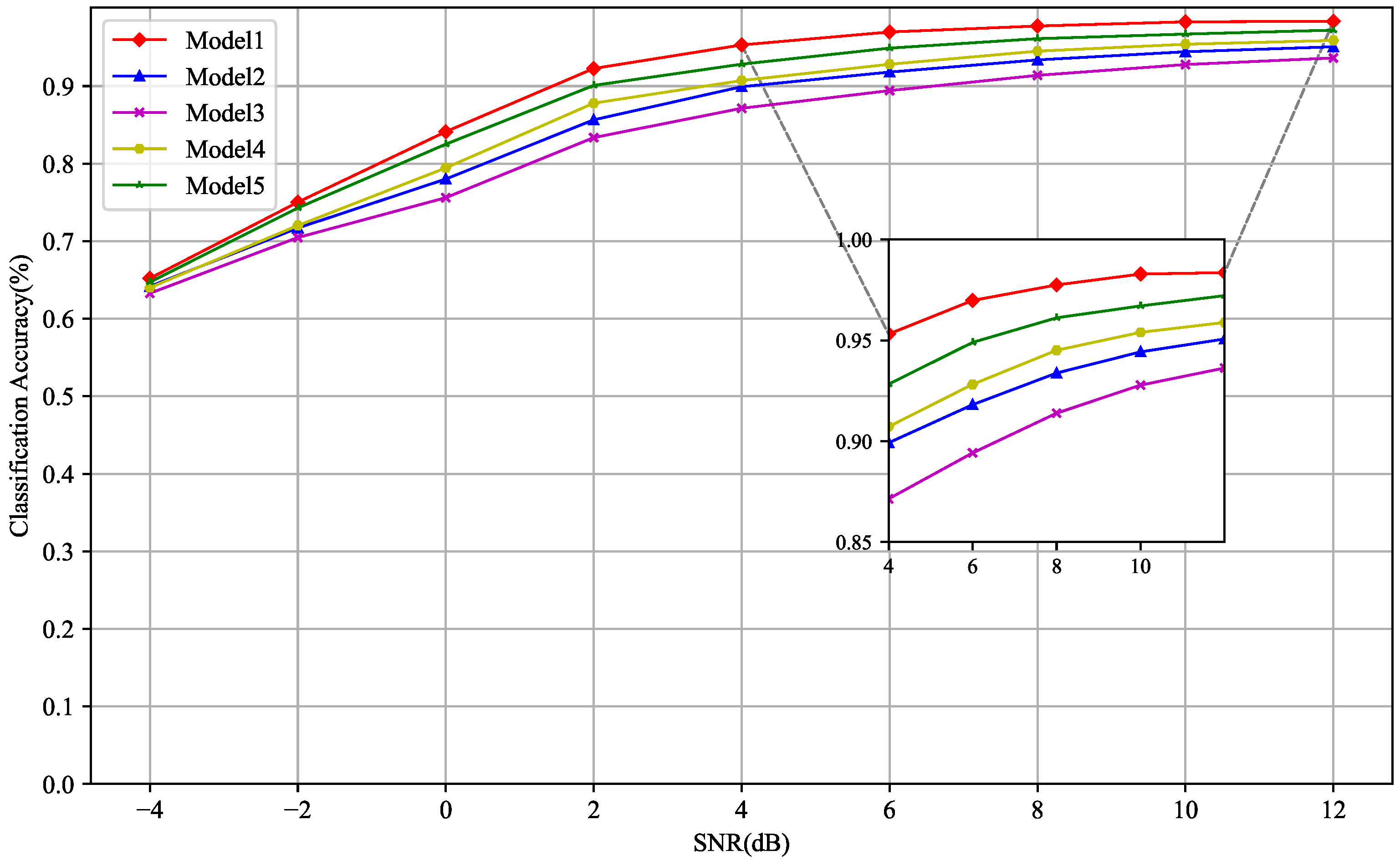
This experiment was conducted on a computer platform equipped with an NVIDIA RTX4090 laptop graphics card, NVIDIA Corporation, Santa Clara, CA, USA (16 GB of video memory) and running Windows 11. Model development and training were performed using the Python 3.8 programming language. All the deep learning models were built and implemented using the Keras framework with a TensorFlow back end. The network structure and training process were simulated and tested locally. During training, the Adam optimizer was used for parameter updates to accelerate model convergence and improve generalization performance. The specific network training parameter configurations are shown in Table 3 analysis. By training and testing these models on the same UWA communication dataset, we can quantify the contribution of each module to classification accuracy, verify the synergistic effects between modules, and demonstrate the superiority of the overall algorithm architecture. The model composition is shown in the Table 4.
As shown in Figure 6, the full DA-TFJA model (Model 1) achieves the highest recognition accuracy at an SNR = 12 dB (98.36%). Removing the ATFT (Model 2) reduces the accuracy to 95.07% (−3.29 pp), indicating that the ATFT strengthens the adaptation to time–frequency variability by enabling the network to learn robust features that accommodate frequency drift and time-scale changes during training. Eliminating the TFAM (Model 4) yields an accuracy of 95.89% (−2.47 pp); by jointly computing time-, frequency-, and cross-domain attention weights, the TFAM focuses the model on informative time–frequency regions while suppressing multipath interference and noise. Further ablation of the DPSE from Model 2 (Model 3) decreases the accuracy to 93.63% (−1.44 pp), confirming that DPSE augments the data with delayed and attenuated replicas that enhance robustness to complex multipath channels. Finally, removing the MTFE (Model 5) results in an accuracy of 97.22% (−1.14 pp), indicating that the residual convolutional blocks of the MTFE capture short-term, medium-term, long-term, and frequency-scale features to address multiscale time–frequency variations introduced by augmentation. Collectively, these findings demonstrate that each component contributes distinct, complementary gains in robustness and overall accuracy.

3.1.3. Accuracy Comparison Across Network Models

To verify the performance advantages of this algorithm, in this work, different network models were selected for accuracy comparison. These comparison models cover the current mainstream deep learning architectures and advanced methods designed specifically for modulation classification tasks. The selected comparison networks are typical and representative: recurrent and convolutional neural network (R&CNN) achieves effective integration of spatiotemporal features by fusing recursive structures with convolutional structures, representing the design idea of a hybrid architecture [23]; multi-channel convolutional and LSTM deep neural network (MCLDNN) introduces cellular neural networks and minimum space tree structures, reflecting a special processing strategy for I/Q dual-channel signals [24]; and MCNet uses multiple asymmetric convolution modules to learn complex spatiotemporal nonlinear relationships, demonstrating the innovative development of convolutional networks in feature extraction [25]. In addition, conventional deep learning models such as CNN-LSTM [26], Squeeze-and-excitation network (SENet) [27], and Residual network (ResNet) [28] were selected as benchmarks to comprehensively evaluate the applicability of different technical paths in UWA communication signal recognition tasks.
All comparison models (DA-TFJA, MCNet, MCLDNN, R&CNN, CNN-LSTM, SENet, ResNet) were trained and tested on exactly the same dataset. Specifically, this includes: the same training set/test set split (7:3 ratio); the same SNR range (−4 dB to 12 dB); the same signal types (2FSK, 4FSK, BPSK, QPSK, DSSS, OFDM with 100 samples each); and the same preprocessing pipeline.
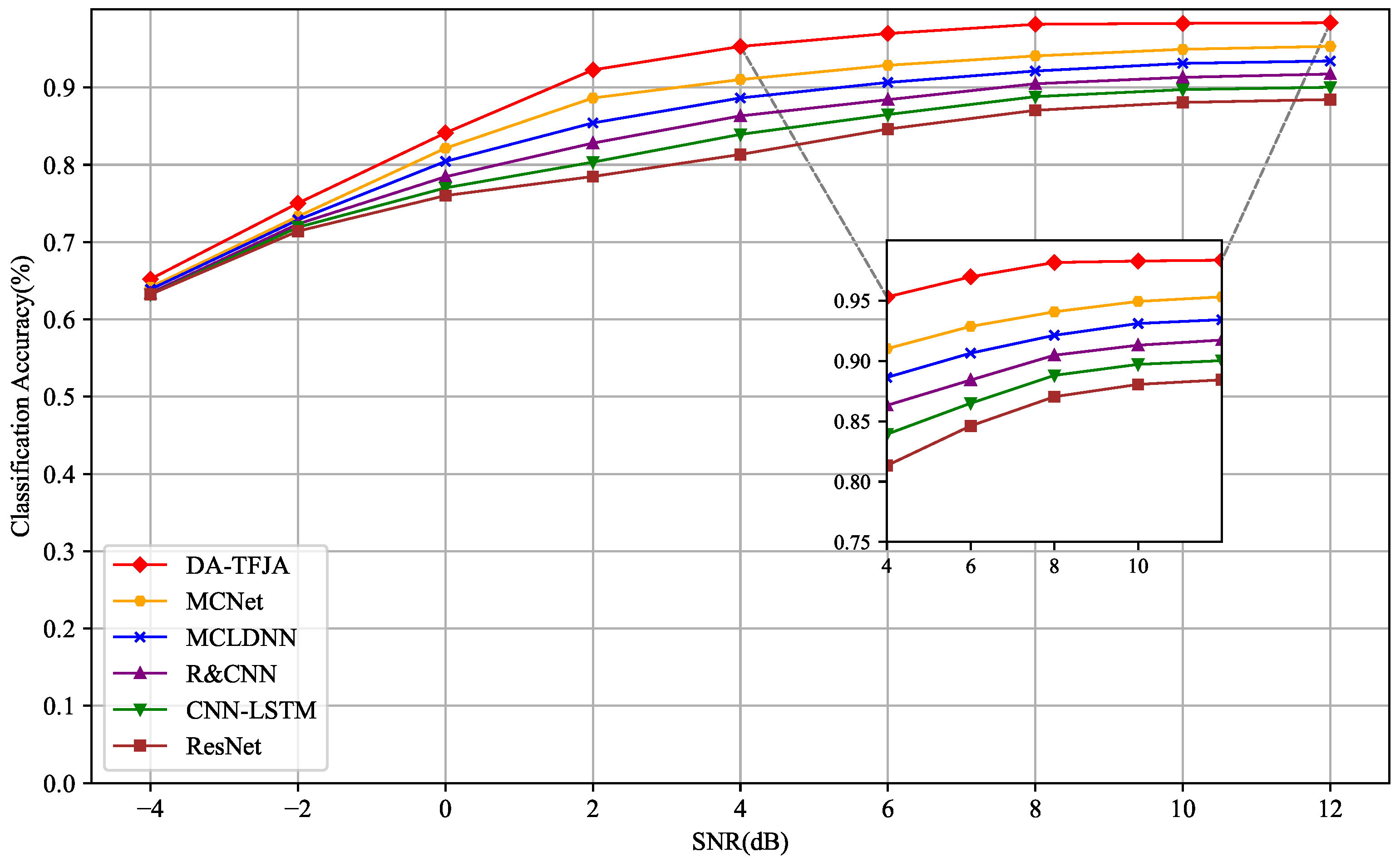
As shown in the Figure 7 the proposed DA-TFJA algorithm demonstrates substantial performance advantages across the entire SNR range. In particular, under high-SNR conditions, it achieves a recognition accuracy of 98.36%, a 3.09-percentage-point improvement over that of the next-best MCNet algorithm. These results underscore the effectiveness of data augmentation and joint time–frequency attention mechanisms. MCNet, with its innovative multigroup asymmetric convolution design, exhibits strong feature extraction under medium- and high-SNR conditions, ultimately achieving a 95.32% accuracy; however, its performance degrades markedly at low SNRs, indicating that relying solely on diverse convolutional architectures is inadequate for robust handling of channel distortion and noise. While the MCLDNN algorithm employs a three-stream parallel architecture to extract complementary features from the I/Q channels, its best accuracy of 93.43% reflects the limitations of straightforward feature-fusion strategies, which fail to fully exploit interchannel synergy. By introducing GRUs for time series preprocessing, the R&CNN algorithm enhances the modeling of time-domain characteristics and achieves a 91.74% recognition rate, surpassing that of the traditional CNN-LSTM combination. This design is consistent with the temporal modeling concept used in this work but lacks a dedicated attention mechanism to highlight key features, resulting in only limited gains. CNN-LSTM, a conventional spatiotemporal feature-extraction framework, is simple and easy to implement, yet its 90.03% accuracy suggests insufficient expressive power for complex modulated signals. Despite the depth and residual connections that should, in principle, endow ResNet with strong representation learning, it attains the lowest recognition rate among all the compared methods (88.44%). These findings suggest that general-purpose deep architectures lacking domain-specific designs—particularly effective modeling of time–frequency features—struggle to achieve optimal performance in UWA communication signal recognition.

3.1.4. Confusion Matrix Analysis at Different Distances

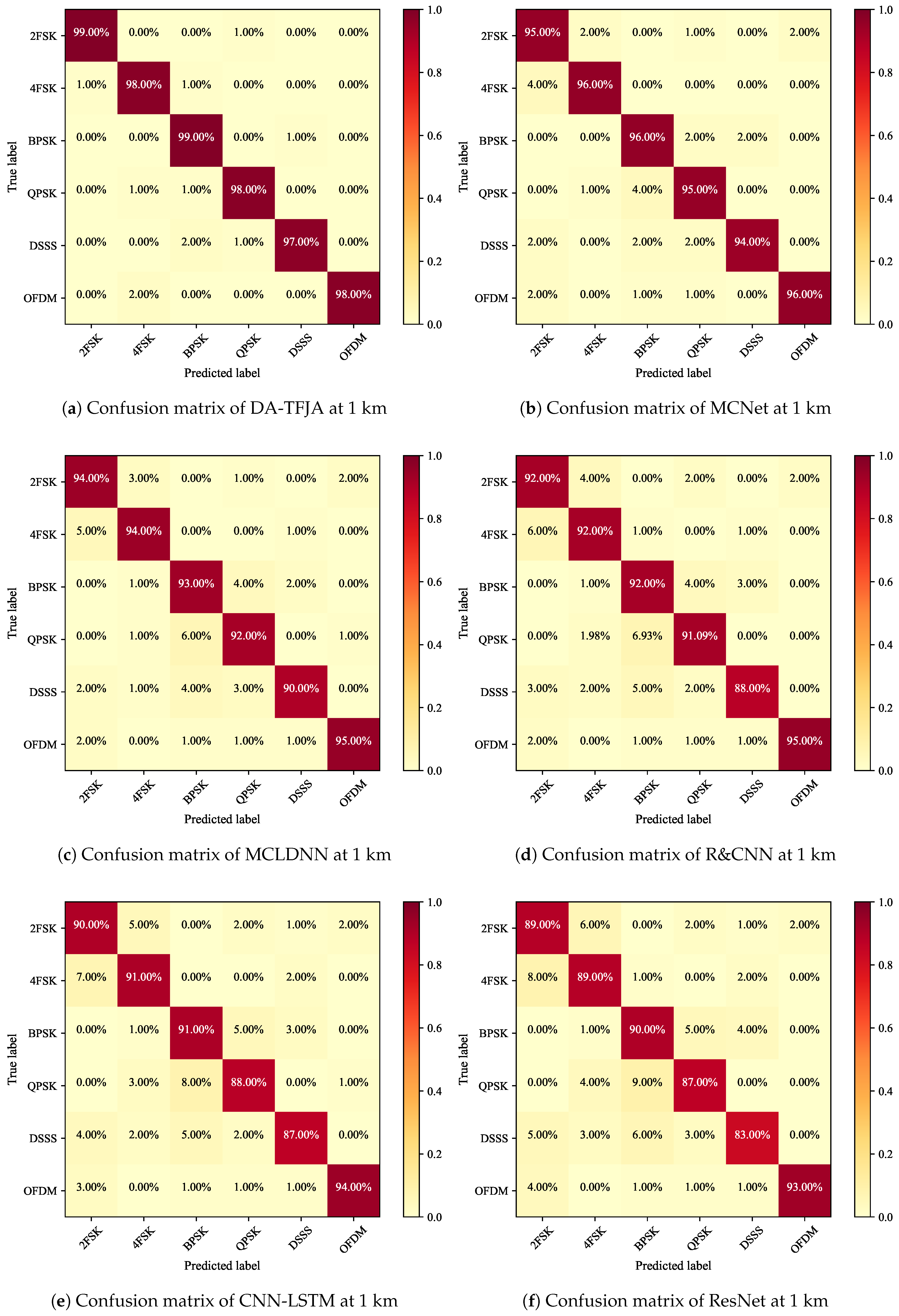
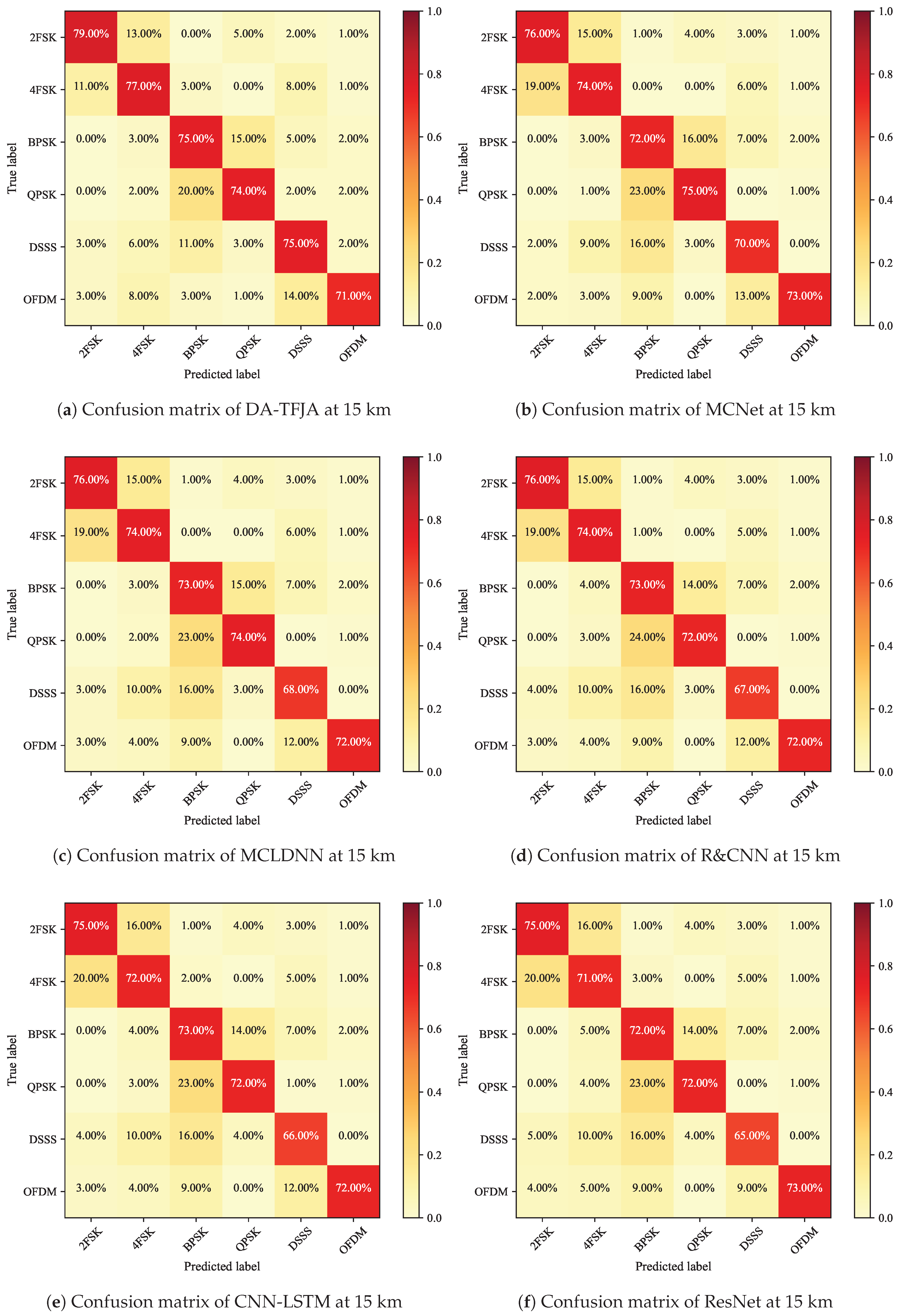
To further analyze the impact of the transmission distance on the performance of the modulation classification algorithms, two typical UWA communication scenarios were designed: short-range (1 km) and long-range (15 km) scenarios. Under these two distance conditions, the proposed DA-TFJA algorithm and five existing benchmark models were used to compare recognition performance. By constructing detailed confusion matrices, the classification accuracy and anti-interference capabilities of the six algorithms were quantitatively evaluated in channel fading environments caused by different transmission distances, as shown in the Figure 8 and Figure 9.
From the confusion matrices in Figure 8, significant performance variations emerge among the six algorithms under the 1-km short-range underwater acoustic channel. The DA-TFJA algorithm (Figure 8a) achieves optimal performance, with all diagonal entries exceeding 97%. Specifically, recognition rates for 2FSK, BPSK, and OFDM reach 99.00%, 99.00%, and 98.00% respectively, exhibiting negligible misclassification. Only DSSS demonstrates minor confusion (2.00%). MCNet (Figure 8b), the second-best performer (95.32% accuracy), shows notably lower recognition rates for 4FSK (96.00%) and DSSS (94.00%) compared to DA-TFJA. A 4.00% confusion between BPSK and QPSK indicates limited discrimination capability for phase-modulated waveforms. MCLDNN (Figure 8c) and R&CNN (Figure 8d) yield comparable accuracies (93.43% and 91.74%), yet both exhibit degraded DSSS recognition (90.00% and 88.00%) and elevated BPSK–QPSK confusion (4.00% to 6.93%). CNN-LSTM (Figure 8e) achieves 90.03% accuracy but demonstrates higher misclassification for QPSK (88.00%) and DSSS (87.00%), with BPSK–QPSK confusion reaching 8.00%—revealing deficiencies in temporal feature modeling. ResNet (Figure 8f), the weakest model (88.44% accuracy), shows diagonal entries predominantly below 90.00%. QPSK and DSSS recognition rates drop to 87.00% and 83.00% respectively, with severe BPSK–QPSK confusion (9.00%), demonstrating the inadequacy of standalone residual architectures for underwater acoustic modulation classification.
A comparison of confusion matrices between 1-km and 15-km transmission distances reveals substantial performance degradation across all algorithms as transmission distance increases significantly. From the 15-km scenario confusion matrices in Figure 9, DA-TFJA (Figure 9a) maintains optimal performance, with diagonal entries ranging from 71.00% to 79.00%. Specifically, 2FSK achieves the highest recognition rate at 79.00%, demonstrating superior stability under challenging channel conditions.MCNet (Figure 9b) achieves an overall accuracy of 73.33%, but exhibits degraded performance for QPSK (75.00% recognition rate) and severe BPSK–QPSK confusion (23.00%). The DSSS recognition rate drops to 70.00%, indicating notable performance deterioration.MCLDNN (Figure 9c) and R&CNN (Figure 9d) demonstrate comparable accuracies of 72.87% and 72.34%, respectively. Both algorithms show deficient DSSS recognition (below 68.00%) and elevated BPSK–QPSK confusion rates (23.00% to 24.00%), revealing inadequate feature extraction capability in severe multipath environments.CNN-LSTM (Figure 9e) achieves 71.91% accuracy, with QPSK and 4FSK recognition rates both declining to approximately 72.00% and exhibiting increased misclassification patterns.ResNet (Figure 9f) demonstrates the weakest performance at 71.41% accuracy, with DSSS recognition falling to 65.00%, 4FSK at 71.00%, and persistent BPSK–QPSK confusion of 23.00%.

4. Conclusions

This paper addresses the scarce training samples and insufficient recognition accuracy in complex channel environments encountered in UWA communication signal recognition tasks. A modulated signal classification and recognition algorithm based on DA-TFJA is proposed. With respect to data augmentation, two algorithms are designed: the ATFT and DPSE. These algorithms simulate the characteristics of realistic UWA channels from the perspectives of time–frequency domain variations and multipath propagation. Signal distortion caused by relative motion between the transmitter and receiver and device asynchrony is effectively simulated by the ATFT through time-domain Doppler transform and frequency-domain carrier offset. Multipath propagation effects caused by reflections from interfaces such as the seabed and surface are realistically reproduced by the DPSE through the dynamic generation of multipath parameters and signal superposition. The diversity of training data is significantly increased and the model’s generalization ability is improved by these two enhancement algorithms. With respect to the network architecture, an end-to-end recognition network that integrates an MTFE, two-layer LSTM temporal modeling, and a TFAM is constructed. Feature information at different time and frequency scales is captured by the MTFE through a four-branch parallel convolutional structure. Intelligent recognition and enhancement of key time–frequency domain information is achieved by the TFAM through the adaptive fusion of time, frequency, and cross-attention. The experimental results reveal that a recognition accuracy of 98.36% on the reservoir-measured dataset is achieved by the algorithm, representing an improvement of 3.09 percentage points compared with the highest recognition rate among the comparison networks. Furthermore, in a noisy environment with an SNR of −4 dB, a signal recognition rate of 65.21% is reached, fully verifying the algorithm’s practical value. Important technical support for the intelligent development of UWA communication systems is provided by the results of this study, and broad application prospects are demonstrated.

Author Contributions

Conceptualization, M.C. and Q.C.; methodology, M.C.; software, M.C.; validation, M.C., Q.C. and J.T., H.W.; formal analysis, M.C.; investigation, M.C.; resources, Q.C.; data curation, M.C.; writing—original draft preparation, M.C.; writing—review and editing, M.C., Q.C. and J.T., H.W.; visualization, M.C.; supervision, J.T. and H.W.; project administration, M.C.; funding acquisition, Q.C. All authors have read and agreed to the published version of the manuscript.

Funding

This research received no external funding.

Data Availability Statement

The raw research data contain sensitive personal information and cannot be shared publicly due to privacy protection regulations (e.g., GDPR/HIPAA). De-identified aggregated datasets supporting the findings of this study are available from the corresponding author upon reasonable request, subject to ethics committee approval and data use agreements.

Acknowledgments

We gratefully acknowledge the hard work and dedication of each author.

Conflicts of Interest

The authors declare no conflicts of interest.

Abbreviations

The following abbreviations are used in this manuscript:
UWAUnderwater acoustic
DA-TFJAData augmentation and time–frequency joint attention
ATFEAdaptive time–frequency transform enhancement algorithm
DPSEDynamic path superposition enhancement algorithm
MTFEMultiscale time–frequency feature extractor
TFAMTime–frequency joint attention mechanism
LSTMLong short-term memory
GANGenerative adversarial network
AMCAutomatic modulation classification
SNRSignal-to-noise ratios
CFOCarrier frequency offset
R&CNNRecurrent and convolutional neural network
MCLDNNMulti-channel convolutional and LSTM deep neural network
SENetSqueeze-and-excitation network
ResNetResidual network
DFTDiscrete fourier transform

References

  1. Wang, Y.; Shen, T.; Wang, T.; Qiao, G.; Zhou, F. Modulation recognition for underwater acoustic communication based on hybrid neural network and feature fusion. Appl. Acoust. 2024, 225, 110185. [Google Scholar] [CrossRef]
  2. Wang, Y.; Xiao, J.; Cheng, X.; Wei, Q.; Tang, N. Underwater acoustic signal classification based on a spatial–temporal fusion neural network. Front. Mar. Sci. 2024, 11, 1331717. [Google Scholar] [CrossRef]
  3. Yao, Q.; Wang, Y.; Yang, Y. Underwater Acoustic Target Recognition Based on Data Augmentation and Residual CNN. Electronics 2023, 12, 1206. [Google Scholar] [CrossRef]
  4. Zhou, F.; Wu, H.; Yue, Z.; Li, H. An Underwater Acoustic Communication Signal Modulation-Style Recognition Algorithm Based on Dual-Feature Fusion and ResNet–Transformer Dual-Model Fusion. Appl. Sci. 2025, 15, 6234. [Google Scholar] [CrossRef]
  5. Wang, B.; Yang, H.; Fang, T. Modulation recognition of underwater acoustic communication signals based on deep learning. Eurasip J. Adv. Signal Process. 2024, 2024, 103. [Google Scholar] [CrossRef]
  6. Xu, M.; Yoon, S.; Fuentes, A.; Park, D.S. A Comprehensive Survey of Image Augmentation Techniques for Deep Learning. Pattern Recognit. 2023, 137, 109347. [Google Scholar] [CrossRef]
  7. Shafiq, M.; Gu, Z. Deep Residual Learning for Image Recognition: A Survey. Appl. Sci. 2022, 12, 8972. [Google Scholar] [CrossRef]
  8. Hendrycks, D.; Mu, N.; Cubuk, E.D.; Zoph, B.; Gilmer, J.; Lakshminarayanan, B. AugMix: A Simple Data Processing Method to Improve Robustness and Uncertainty. arXiv 2020, arXiv:1912.02781. [Google Scholar] [CrossRef]
  9. Cubuk, E.D.; Zoph, B.; Shlens, J.; Le, Q.V. RandAugment: Practical Automated Data Augmentation with a Reduced Search Space. In Advances in Neural Information Processing Systems 33, NEURIPS 2020, Proceedings of the 34th Conference on Neural Information Processing Systems (NeurIPS), Electr Network, New Orleans, LA, USA, 10–16 December 2020; Larochelle, H., Ranzato, M., Hadsell, R., Balcan, M., Lin, H., Eds.; Curran Associates, Inc.: Red Hook, NY, USA, 2020; Volume 33. [Google Scholar]
  10. DeVries, T.; Taylor, G.W. Improved Regularization of Convolutional Neural Networks with Cutout. arXiv 2017, arXiv:1708.04552. [Google Scholar] [CrossRef]
  11. Zhong, Z.; Zheng, L.; Kang, G.; Li, S.; Yang, Y. Random Erasing Data Augmentation. In AAAI Conference on Artificial Intelligence, Proceedings of the 34th AAAI Conference on Artificial Intelligence/32nd Innovative Applications of Artificial Intelligence Conference/10th AAAI Symposium on Educational Advances in Artificial Intelligence, New York, NY, USA, 7–12 February 2020; Association for the Advancement of Artificial Intelligence: Palo Alto, CA, USA, 2020; Volume 34, pp. 13001–13008. [Google Scholar]
  12. Radford, A.; Metz, L.; Chintala, S. Unsupervised Representation Learning with Deep Convolutional Generative Adversarial Networks. arXiv 2016. [Google Scholar] [CrossRef]
  13. Karras, T.; Laine, S.; Aila, T. A Style-Based Generator Architecture for Generative Adversarial Networks. In Proceedings of the IEEE/CVF Conference on Computer Vision and Pattern Recognition (CVPR), Long Beach, CA, USA, 15–20 June 2019. [Google Scholar]
  14. Peng, Y.; Hou, C.; Zhang, Y.; Lin, Y.; Gui, G.; Gacanin, H.; Mao, S.; Adachi, F. Supervised Contrastive Learning for RFF Identification With Limited Samples. IEEE Internet Things J. 2023, 10, 17293–17306. [Google Scholar] [CrossRef]
  15. Yin, L.; Xiang, X.; Liang, Y.; Liu, K. Modulation classification with data augmentation based on a semi-supervised generative model. Wirel. Netw. 2024, 30, 5683–5696. [Google Scholar] [CrossRef]
  16. Wang, N.; Liu, Y.; Ma, L.; Yang, Y.; Wang, H. Automatic Modulation Classification Based on CNN and Multiple Kernel Maximum Mean Discrepancy. Electronics 2023, 12, 66. [Google Scholar] [CrossRef]
  17. Gong, A.; Zhang, X.; Wang, Y.; Zhang, Y.; Li, M. Hybrid Data Augmentation and Dual-Stream Spatiotemporal Fusion Neural Network for Automatic Modulation Classification in Drone Communications. Drones 2023, 7, 346. [Google Scholar] [CrossRef]
  18. Shen, W.; Xu, D.; Xu, X.; Chen, Z.; Xuan, Q.; Wang, W.; Lin, Y.; Yang, X. A simple data augmentation method for automatic modulation recognition via mixing signals. In Proceedings of the 2024 6th International Conference on Robotics, Intelligent Control and Artificial Intelligence (RICAI), Nanjing, China, 6–8 December 2024; pp. 219–229. [Google Scholar] [CrossRef]
  19. Li, M.; Wang, P.; Dong, Y.; Wang, Z. Diffusion Model Empowered Data Augmentation for Automatic Modulation Recognition. IEEE Wirel. Commun. Lett. 2025, 14, 1224–1228. [Google Scholar] [CrossRef]
  20. Li, D.; Liu, F.; Shen, T.; Chen, L.; Zhao, D. Data augmentation method for underwater acoustic target recognition based on underwater acoustic channel modeling and transfer learning. Appl. Acoust. 2023, 208, 109344. [Google Scholar] [CrossRef]
  21. Ramya, S.; Hema, L.K.; Jenitha, J.; Regilan, S. Deep Learning-Driven Autoencoder Models for Robust Underwater Acoustic Communication: A Survey on DCAEs, VAEs, Adaptive Modulation. In Proceedings of the 2025 11th International Conference on Communication and Signal Processing (ICCSP), Melmaruvathur, India, 5–7 June 2025; pp. 771–776. [Google Scholar] [CrossRef]
  22. Feng, Y.; Chen, Z.; Chen, Y.; Xie, Z.; He, J.; Li, J.; Ding, H.; Guo, T.; Chen, K. LW-MS-LFTFNet: A Lightweight Multi-Scale Network Integrating Low-Frequency Temporal Features for Ship-Radiated Noise Recognition. J. Mar. Sci. Eng. 2025, 13, 2073. [Google Scholar] [CrossRef]
  23. Zhang, W.; Yang, X.; Leng, C.; Wang, J.; Mao, S. Modulation Recognition of Underwater Acoustic Signals Using Deep Hybrid Neural Networks. IEEE Trans. Wirel. Commun. 2022, 21, 5977–5988. [Google Scholar] [CrossRef]
  24. Xu, J.; Luo, C.; Parr, G.; Luo, Y. A Spatiotemporal Multi-Channel Learning Framework for Automatic Modulation Recognition. IEEE Wirel. Commun. Lett. 2020, 9, 1629–1632. [Google Scholar] [CrossRef]
  25. Huynh-The, T.; Hua, C.H.; Pham, Q.V.; Kim, D.S. MCNet: An Efficient CNN Architecture for Robust Automatic Modulation Classification. IEEE Commun. Lett. 2020, 24, 811–815. [Google Scholar] [CrossRef]
  26. Zhang, Z.; Luo, H.; Wang, C.; Gan, C.; Xiang, Y. Automatic Modulation Classification Using CNN-LSTM Based Dual-Stream Structure. IEEE Trans. Veh. Technol. 2020, 69, 13521–13531. [Google Scholar] [CrossRef]
  27. Hu, J.; Shen, L.; Sun, G. Squeeze-and-Excitation Networks. In Proceedings of the IEEE Conference on Computer Vision and Pattern Recognition (CVPR), Salt Lake City, UT, USA, 18–23 June 2018. [Google Scholar]
  28. O’Shea, T.J.; Roy, T.; Clancy, T.C. Over-the-Air Deep Learning Based Radio Signal Classification. IEEE J. Sel. Top. Signal Process. 2018, 12, 168–179. [Google Scholar] [CrossRef]
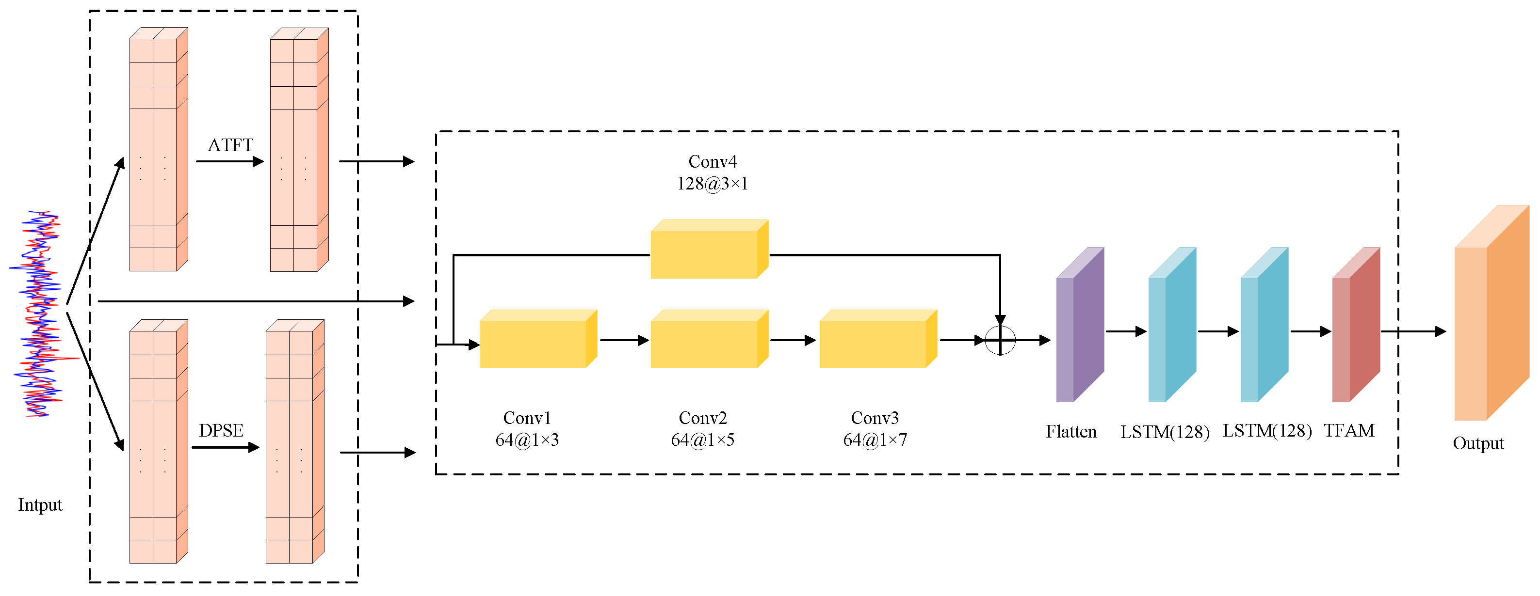
Figure 1. Overall algorithm design.
Jmse 14 00172 g001
Figure 2. The structure of ATFT.
Jmse 14 00172 g002
Figure 3. The structure of DPSE.
Jmse 14 00172 g003
Figure 4. The structure of Feature extraction network.
Jmse 14 00172 g004
Figure 5. The structure of MTFE.
Jmse 14 00172 g005
Figure 6. Ablation study.
Jmse 14 00172 g006
Figure 7. Recognition accuracy under different network models.
Jmse 14 00172 g007
Figure 8. Comparison of confusion matrices at 1 km.
Jmse 14 00172 g008
Figure 9. Comparison of confusion matrices at 15 km.
Jmse 14 00172 g009
Table 1. Summary of existing data augmentation methods for automatic modulation classification.
ReferenceMethodAdvantagesDisadvantages
Peng, Y. et al. [14]Constellation diagram rotationEnhances robustness to phase changesInsufficient constellation diagram data remains
Yin, L. et al. [15]GAN-based constellation generationEffectively improves model generalization abilityGenerated samples may lack authenticity; high computational complexity
Wang, N. et al. [16]Signal rotation with RandMix strategyProvides powerful solution to domain shift problem in AMCComputational complexity too high for practical applications
Gong, A. et al. [17]I/Q and A/P fusion with rotation and self-perturbationImproves adaptability to complex environmentsLimited recognition rate improvement for specific modulation types
Shen, W. et al. [18]Mixed-signal augmentation frameworkEffectively improves modulation classification accuracyDestroys temporal dependency; introduces noise or incorrect learning patterns
Li, M. et al. [19]Conditional diffusion modelGenerates high-fidelity and diverse signal samples; solves training data insufficiencyHigh computational requirements; not optimized for UWA characteristics
Table 2. Signal parameters.
Signal TypeCarrier
Frequency
(kHz)
Signal
Bandwidth
(kHz)
Duration
(/s)
Signal
Count
PN Code
Order
Number of
Subcarriers
2FSK7.521100
4FSK7.521100
BPSK7.521100
QPSK7.521100
DSSS7.5211005
OFDM7.521100512
Table 3. Training Parameter Settings.
Parameter SettingsValue
Epochs120
Batch Size512
OptimizerAdam
Learning Rate0.001
Patience15
Dropout0.5
Table 4. Modules of the network model.
ModelATFTDPSEMTFETFAM
Model 1
Model 2
Model 3
Model 4
Model 5
Disclaimer/Publisher’s Note: The statements, opinions and data contained in all publications are solely those of the individual author(s) and contributor(s) and not of MDPI and/or the editor(s). MDPI and/or the editor(s) disclaim responsibility for any injury to people or property resulting from any ideas, methods, instructions or products referred to in the content.