Path Planning of an Underwater Vehicle by CFD Numerical Simulation Combined with a Migration-Based Genetic Algorithm

Abstract

This paper proposes a physics-informed global path planning framework for underwater vehicles integrating CFD simulation and the genetic algorithm. The CFD simulation models the flow field along the planned path of the underwater vehicle. The current velocity data are incorporated into the following path planning that is based on an improved genetic algorithm (GA), which uses migration operators to share the information about feasible solutions or paths, improving the fitness of the whole population. In the three steps of the GA procedure, an elite selection strategy is adopted to avoid losing excellent solutions. A segmented crossover strategy is adopted to avoid low-quality crossover. An adaptive mutation strategy is used to enhance the ability to escape a local optimal solution. Using the improved GA, single-target and multi-target underwater path planning are investigated. In multi-target path planning, a combined algorithm is proposed to solve the optimal traversal order of target points and plan a feasible path between target points. The simulation results show that the proposed algorithm has good planning ability for both simple and complex underwater scenarios. Compared with the conventional GA and an improved GA, the number of average iterations decreases by 45.3% and 29.9%, respectively, for 2D multi-target path planning. The number of average inflection points decreases by 50.3% and 44.2%, respectively, for 2D multi-target path planning.

1. Introduction

Underwater vehicles are important tools for humans to explore and exploit oceans. To fulfill assigned missions in complicated underwater environments, autonomy and safety should be guaranteed, which can be achieved by well-designed controllers. Point stabilization, path following, and trajectory tracking are usually the main concerns in controller design for underwater vehicles. For the latter two, path planning is a process that greatly affects controller performance. Path planning allows an underwater vehicle to find the shortest and most obstacle-free path from the start to goal. During the last decades, the path planning of underwater vehicles has been given constant attention. Various algorithms have been proposed. Conventional algorithms include Dijkstra’s algorithm, the A* algorithm, RRT algorithm, etc. Dijkstra’s algorithm is a classic method used to solve shortest path problems. It employs a greedy strategy to guarantee the optimal solution at each step [1]. However, for high-dimensional problems, the increase in the number of nodes might lead to extra planning time. Therefore, Dijkstra’s algorithm is better suited for global planning scenarios where real-time requirements are not critical. Guo et al. [2] improved Dijkstra’s algorithm by retaining nodes equidistant from all source nodes, thus increasing the number of alternative nodes for the next step. In this way, an optimal path with the shortest travel time is successfully planned. Gu et al. [3] combined Dijkstra’s algorithm with time windows in the path planning for magnetic levitation vehicles. A reduction in the total time required for orders is achieved while ensuring conflict-free operations. Zhang et al. [4] extended the path planning space to three dimensions by increasing the search directions of Dijkstra’s algorithm. Dijkstra’s algorithm is inherently designed for static graphs, assuming constant edge weights. This presents a critical shortcoming for path planning in current fields, which are temporally dynamic. The A* algorithm combines the heuristic search with Dijkstra’s algorithm. Instead of expanding nodes in all directions, the A* algorithm prioritizes nodes that are closer to the target [5]. However, with the increase in dimensionality, the planning time of the A* algorithm also increases rapidly. In addition, this algorithm struggles in dynamic environments. Jiang et al. [6] enhanced the traditional A* algorithm by using obstacle rates to adjust the weight of the heuristic function and optimized the nodes. Song et al. [7] addressed the ‘jags’ issue in the traditional A* algorithm by using a smoothing strategy to obtain smoother and more reasonable planned paths. Richter et al. [8] proposed a global planning algorithm based on the A* algorithm. Similar to Dijkstra’s algorithm, the performance of A* is critically limited by the difficulty in designing effective time-varying heuristic functions, while also confronting the challenge of changes in time and space. The RRT algorithm is a sampling-based method that is strongly applicable in high-dimensional spaces and complex environments. By random sampling, it rapidly explores the space. By mimicking the random growth of a tree, it expands incrementally until the target is reached [9]. However, the paths generated by the RRT algorithm are generally not optimal. Du et al. [10] introduced a node gravitational field function to reduce the generation of invalid nodes and employed B-spline curves to improve the smoothness in RRT-based planning. Ruan et al. [11] proposed an improved RRT algorithm, in which four random trees are constructed for searching and an adaptive strategy is designed for generating new nodes to reduce the probability of the algorithm being trapped in local optima. By replacing traditional random sampling with heuristic sampling, Jiang et al. [12] significantly enhances the RRT algorithm’s efficiency. The main value of the RRT series of algorithms in complex water flow environments lies in their powerful obstacle avoidance and global exploration capabilities. However, they have serious weaknesses: inherent randomness, non-smooth paths, and clumsy handling of dynamic environments.

With the development of artificial intelligence (AI), new approaches are available to the path planning of marine vehicles, including the genetic algorithm (GA) [13,14], ant colony algorithm (ACA) [15,16], biogeography-based optimization algorithm (BBOA) [17,18], Whale Optimization Algorithm (WOA) [19,20], Grey Wolf Optimizer (GWO) [21,22], deep reinforcement learning (DRL) [23,24], etc. Among the AI technique-based path planning strategies, GA is widely used since it is straightforward in principle and easily integrates with other algorithms. By tailoring the factors of GA for path planning problems, Li et al. [13] employed fuzzy logic control to adjust the crossover and mutation probabilities. The algorithm’s applicability was validated through simulations in both static and dynamic environments. Zhang et al. [14] adopted adaptive adjustment of crossover and mutation probabilities, effectively enhancing the planning capability of the improved algorithm. Despite its wide application, GA tends to perform poorly and produce unstable optimization results in complex environments. Wang et al. [25] proposed an improved GA that can automatically adjust the crossover probability and mutation probability according to the change in the fitness value in the evolutionary process, avoiding local optimal solutions and prematurity. Zhang et al. applied a non-dominated sorting GA to the path planning of an underwater glider [26].

To address the issues of slow convergence speed and susceptibility to local optima in traditional GAs for underwater vehicle path planning, this paper proposes an improved genetic algorithm by incorporating the migration concept from the biogeography-based optimization algorithm. The feasibility of the proposed genetic algorithm combined with migration (GAM) is validated through multiple sets of comparative experiments. Compared with the Biogeography-Based Optimization Algorithm (BBOA) proposed in [17,18], we have introduced a different “change_path” operator that integrates intersection-based path crossover and a heuristic bridging mechanism, offering greater efficiency and robustness than traditional BBO migration. When an inferior path shares nodes with an elite path, our proposed operator does not perform random component migration. Instead, it executes topology-aware path crossover. This is equivalent to directly grafting the “wisdom of the latter segment” from the elite path onto the inferior one. This design offers three advantages: (1) maintaining path continuity; (2) inheriting validated feasible segments; and (3) facilitating efficient learning. To address the potential failure of traditional BBO when no common nodes exist, we designed a heuristic bridging mechanism. It randomly extracts a front segment from the inferior path and makes multiple attempts to connect it to a node on the elite path. We also incorporated a “remove-loops” operator to eliminate redundant cycles. Our method ensures the stability and robustness of the migration operation, preventing population degradation that may arise from traditional migration. For environmental modeling, traditional methods adopt empirical formulas to describe the underwater environment, for example, the Lamb model used for current modeling [27], streamfunction [28], and constant current model [22]. Although empirical formulas are characterized by simple calculation, the accuracy and feasibility need to be improved. In fact, the complex flow field around obstacles exerts a great impact on the motion of underwater vehicles and the reachability of the planned path. In this study, the CFD technique is employed to analyze the flow field distribution. Nowadays, CFD has found wide application in many engineering areas owing to its powerful calculation ability. In this paper, the proposed GAM is used for the path planning of an underwater vehicle under a CFD-based environment model. Both single-target and multi-target path planning are investigated. The contributions of the study include the following: (1) An improved genetic algorithm combined with migration (GAM) is proposed. This algorithm uses migration operators to share information about feasible solutions, improving the fitness of the whole system. (2) CFD numerical simulation is conducted to obtain flow information that helps the path planning algorithm avoid infeasible paths. (3) For multi-target path planning, a combinatorial planning algorithm is proposed which simultaneously considers the traversal order of multiple target points and the feasible paths between the target points.

The rest of the paper is organized as follows. In Section 2, the fundamentals on the environment modeling, genetic algorithm, and CFD calculation are given; in Section 3, the improved genetic algorithm and its combination with flow field are described; in Section 4, a simulation is conducted to verify the proposed path planning strategy; and in the final section, conclusions are given.

2. Materials and Methods

2.1. Environment Modeling

In the procedure of a path planning task, a reasonable representation of scenario, i.e., environmental modeling, is essential. Environmental modeling converts the information about the task area into a mathematical model that facilitates problem-solving, thus reducing the computational load of the path planning algorithm. Commonly used environmental modeling methods include the visibility graph method, topology method, and grid method. Comparatively, the grid method is simpler for creating maps. It can quickly generate information about the environmental area and update the map when the environment changes. In this study, the grid method is employed to the modeling of the working environment of the underwater vehicle. The operational area is divided into n × n grids. Each grid is numbered following the sequence from left to right and bottom to top. The path to be planned consists of multiple feasible grids. The relationship between the grid number and its corresponding coordinate in the two-dimensional grid map is given as follows [29]:

$$\left\{\begin{array}{l}{N}_x=mod\left(Num,X\right)+1\\ N_y=fix\left(Num,Y\right)+1\end{array}\right.$$

(1)

where $Num$ is the assigned number of the grid, X represents the dimension of the grid map in the x-direction, Y represents the dimension in the y-direction, N_x is the x-coordinate of the grid on the map, and N_y is the y-coordinate. The mod(·) function is used to calculate the remainder, while the fix(·) function is used to round towards zero.

2.2. Genetic Algorithm

The genetic algorithm (GA) is an intelligent optimization algorithm. It creates models by simulating the survival of the fittest and biological evolution processes in nature. GA has been one of the most important and successful algorithms in optimization, as demonstrated by numerous applications. With the advancement of computational capabilities, GA is able to solve increasingly sophisticated problems, in both research and practical domains.

A standard genetic algorithm usually consists of three operators, i.e., selection, crossover, and mutation operators. The selection operation is to identify high-fitness individuals within the population, ensuring that high-quality solutions from the parent generation are preserved. The crossover operation is a critical aspect of biological genetic evolution since it is the primary way to generate new offspring. As iterations proceed, population diversity gradually decreases, which is the main cause of local optima. Therefore, the mutation operation is conducted. This operation randomly selects certain genes within an individual’s chromosome for mutation to generate new individuals, thus enhancing population diversity and enabling the algorithm to escape local optima.

2.3. Computational Fluid Dynamics

For an underwater vehicle that works in oceanic environments, the influence of flow fields on the planned path should be taken into account. When an underwater vehicle moves against strong currents, it is difficult to reach the target point successfully even if the planned path is theoretically optimal. This paper constructs a flow field database for an underwater vehicle by using computational fluid dynamics (CFD) numerical simulations. The information about the flow field is integrated into the environmental model, and the feasibility of the path planning algorithm for the underwater vehicle is verified.

CFD simulation strategies mainly include direct numerical simulation (DNS), large eddy simulation (LES) and the Reynolds-average Navier Stokes (RANS) simulation. In this study, the RANS method is used owing to its calculation efficiency.

3. Path Planning Based on GAM

3.1. Genetic Algorithm Combined with Migration

In traditional genetic algorithms to solve path planning problems, the initial population is often generated randomly. It tends to produce initial populations with numerous redundant nodes and may even produce infeasible grids, especially when obstacles are large. To enhance the quality of population initialization, this paper adopts the following approach. First, excluding the rows containing the start and end points, a feasible grid is randomly selected in each row in ascending order. Combined with the start and end points, these selected grids form a node sequence for the path. Subsequently, the continuity between adjacent nodes in the sequence within the grid environment is evaluated on the following basis:

$$O=\max \left\{\left|x_{i+1}-x_i\right|,\left|y_{i+1}-y_i\right|\right\}$$

(2)

where $\left(x_i,y_i\right)$ and $\left(x_{i+1},y_{i+1}\right)$ represent the coordinates of the corresponding node in the sequence. If the value of O is one, it indicates that the adjacent nodes in the sequence are continuous. Otherwise, feasible nodes will be added to form an uninterrupted continuous path sequence. To this end, the following mean value interpolation method is employed.

$$\left\{\begin{array}{l}{x}_{new}=floor\left({\displaystyle \frac{x_{i+1}+x_i}{2}}\right)\\ y_{new}=floor\left({\displaystyle \frac{y_{i+1}+y_i}{2}}\right)\end{array}\right.$$

(3)

where $\left(x_{new},y_{new}\right)$ is the node to be added; and floor(·) denotes the floor function. In the case where $\left(x_{new},y_{new}\right)$ is an obstacle grid, feasible nodes around it should be selected. Through multiple iterations, a continuous sequence of path nodes is generated to complete the initialization of the population.

To enhance the overall fitness of the population, migration is performed. This operation enables different feasible solutions to share information so that inferior feasible solutions learn from superior ones. The immigration and emigration rates are calculated as follows [17]:

$$\left\{\begin{array}{l}{\lambda }_i=I\times \left(I-{\displaystyle \frac{S_i}{S_{\max }}}\right)\\ {\mu }_i=E\times {\displaystyle \frac{S_i}{S_{\max }}}\end{array}\right.$$

(4)

where ${\lambda }_i$ is the immigration rate; ${\mu }_i$ is the emigration rate; I is the maximum possible immigration rate; E is the maximum possible emigration rate; and S_max is the largest possible number of species.

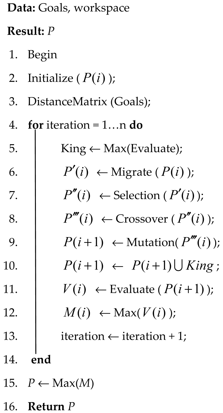
The pseudo-code of the proposed genetic algorithm combined with the migration (GAM) algorithm is shown in Algorithm 1. First, the initialization of population is performed. The obtained feasible solutions form a sequence of grid nodes. The fitness value of these feasible solutions is calculated by using a Euclidean distance-based evaluation function. Next, an elitist preservation strategy is employed. The feasible solution with the highest fitness value is selected and does not participate in subsequent operations. Afterwards, the migration operation is conducted to improve the fitness values of feasible solutions. The immigration and emigration rates are calculated and the paths for immigration and emigration are selected using the roulette wheel method. In the crossover stage, a random number within the range [0, 1] is generated to determine whether a crossover operation should be performed. The population is divided into three parts according to the fitness values and crossover is conducted within the same parts to reduce low-quality crossovers. First, all feasible solutions are ranked by their fitness values. Based on this ranking, they are categorized into three groups (good, medium, poor). Subsequently, within the same group, two feasible solutions are selected. A common node (excluding the start and end points) is randomly chosen as the crossover node to exchange their path segments. These solutions of intra-group crossover inherently impose a degree of constraint on the search direction. Compared to the traditional genetic algorithm, where two solutions are randomly selected from the entire population for crossover, our method substantially reduces the generation of low-quality offspring, thereby accelerating the convergence rate. Similar to the crossover operation, mutation is executed when the regenerated random number is less than the mutation probability. The population is sorted by fitness values. The top fifth is classified as elite solutions that do not undergo mutation, while the remaining solutions undergo mutation. Following the mutation stage, the fitness values of the population are updated and the optimal solution is recorded. When the maximum number of iterations has been reached, the iteration stops and the optimal path is obtained.

Traditional GA initializes paths through pure randomness, resulting in a low probability of feasible paths near large obstacles and computationally wasteful repair attempts. Our method overcomes this by directly generating a higher-quality initial population, requiring no repair. The design is two-fold: row-by-row progression provides macro-directional bias from start to goal, avoiding local traps; and in-row randomization preserves micro-level exploration as a form of constrained randomness. Path diversity will be further supplemented by subsequent migration, mutation, and crossover operations.

In Algorithm 1, Evaluate(P(i)) refers to the calculation of the fitness value for each path in the i-th population generation using the path fitness function E (Equation (5)). The evaluation criteria for the quality of a planned path generally involve multiple aspects such as path length and smoothness, which can be measured by a specific fitness function. In this paper, the primary research metric is the length of the planned path, while smoothness is taken as the secondary metric. As a path is composed of a sequence of nodes, the Euclidean distance is selected to determine the distance between two adjacent nodes. The path fitness function is defined as follows [30]:

$$E={\omega }_1\times D^{-1}+{\omega }_2\times S^{-1}$$

(5)

where ${\omega }_i$ is the weight; D is the Euclidean distance; and S is the cost of path smoothness.

$$D={\displaystyle \sum _{i=1}^{n-1}\sqrt{{\left(x_{i+1}-x_i\right)}^2+{\left(y_{i+1}-y_i\right)}^2}}$$

(6)

where n is the number of nodes.

$$S={\displaystyle \sum _i^{n-2}\left\{\begin{array}{ll}3& angle\in \left(91,136\right]\\ 15& angle\in \left(46,91\right]\\ 200& angle\in \left(0,46\right]\end{array}\right.}$$

(7)

where angle is the angle formed by three adjacent nodes, which can be calculated using the cosine theorem.

Migrate((P(i)) denotes the migration operation applied to the paths generated after the i-th iteration;

$$l_k^{\mathrm{mig}}=\left\{\begin{array}{ll}\mathcal{T}(l_k,\arg {\max }_j\{{\displaystyle \sum _{t=1}^j\mathbb{P}}(t|k)\ge \mathrm{rand}\})\hfill & \mathrm{rand}\le {\lambda }_k\hfill \\ l_k\hfill & \mathrm{otherwise}\hfill \end{array}\right.$$

(8)

where $l_k^{\mathrm{mig}}$ is the new k-th path after undergoing the migration operation; $\mathcal{T}(\cdot )$ is the function of the path generated; and $\arg {\max }_j\{{\displaystyle \sum _{t=1}^j\mathbb{P}}(t|k)\ge \mathrm{rand}\}$ is the j-th path as the migration path through roulette.

Selection(P(i)) represents the selection process for the paths produced in the i-th generation. In this step, the probability of each individual being selected is computed based on its fitness value (higher fitness corresponds to a greater probability). These probabilities are summed to form a cumulative probability distribution over the interval [0, 1]. A random number is then generated, and the individual corresponding to the cumulative probability interval in which this number falls is selected. This process is repeated until the new population reaches the size of the original population, as shown below:

$$P^{″}(i)=\left\{P\min \left.\left\{t\in \left[1,\mathrm{N}\right]\left|ri\right.<{\displaystyle {\sum }_{s=1}^t\frac{ES}{{\displaystyle {\sum }_{k=1}^{N}Ek}}}\right\}\right|\begin{array}{l}i=1,2,3\dots \mathrm{N}\\ r1\le r2\le \dots \le r\mathrm{N}\end{array}\right\}$$

(9)

Crossover(P(i)) performs the crossover operation as follows: First, the population is sorted in descending order based on fitness and then divided into three groups. Within each group, two paths are randomly selected. It is then determined whether these two paths share any common points (excluding the start point and end point). Next, a random number x between 0 and 1 is generated. If x < P_C (predefined probability in crossover operation), a common point is randomly selected and crossover is performed at that point. If x ≥ P_C, no crossover is applied. If the two paths do not share any common points (other than the start and end points), a segment from each path is randomly selected and joined together. If this process fails to produce a valid path after 100 attempts, the original paths are retained to avoid generating invalid solutions.

$$\{l_i^{\mathrm{cross}},l_j^{\mathrm{cross}}\}x<{\mathrm{p}}_{\mathrm{c}}=\mathcal{I} \left(l_{\sigma {(E)}_i},l_{\sigma {(E)}_j},p_c\right)$$

(10)

where $l_i^{\mathrm{cross}}$ and $l_j^{\mathrm{cross}}$ are the i-th and j-th paths within the same group, respectively; and $\mathcal{I} \left(\cdot \right)$ is the Cross-path generation function.

Mutation(P(i)) refers to the mutation operation applied to the paths generated in the i-th iteration. First, all paths are sorted according to their fitness values. The top 1/5 of the paths are preserved without any mutation. For each of the remaining paths, a random number y between 0 and 1 is generated. If y < Pm (predefined probability in mutation operation), a mutation operation—specifically, path segment replacement—is performed on that path; otherwise, no mutation is applied.

$$P(i+1)=\left\{\begin{array}{l}{l}_{\sigma ECi} i\le ceil({\displaystyle \frac{N}{5}})\\ M_{slice}(l_{\sigma ECi}) i\in (ceil({\displaystyle \frac{N}{5}})),if y<Pm \end{array}\right\}$$

(11)

where $l_{\sigma ECi}$ are the paths within the top fifth of the fitness values; and $Mslice(\cdot )$ is the function that path generated after mutating; P(i) denotes the path generated after the i-th iteration, while P denotes the path with the highest fitness value after 50 iterations.

Algorithm 1: GAM

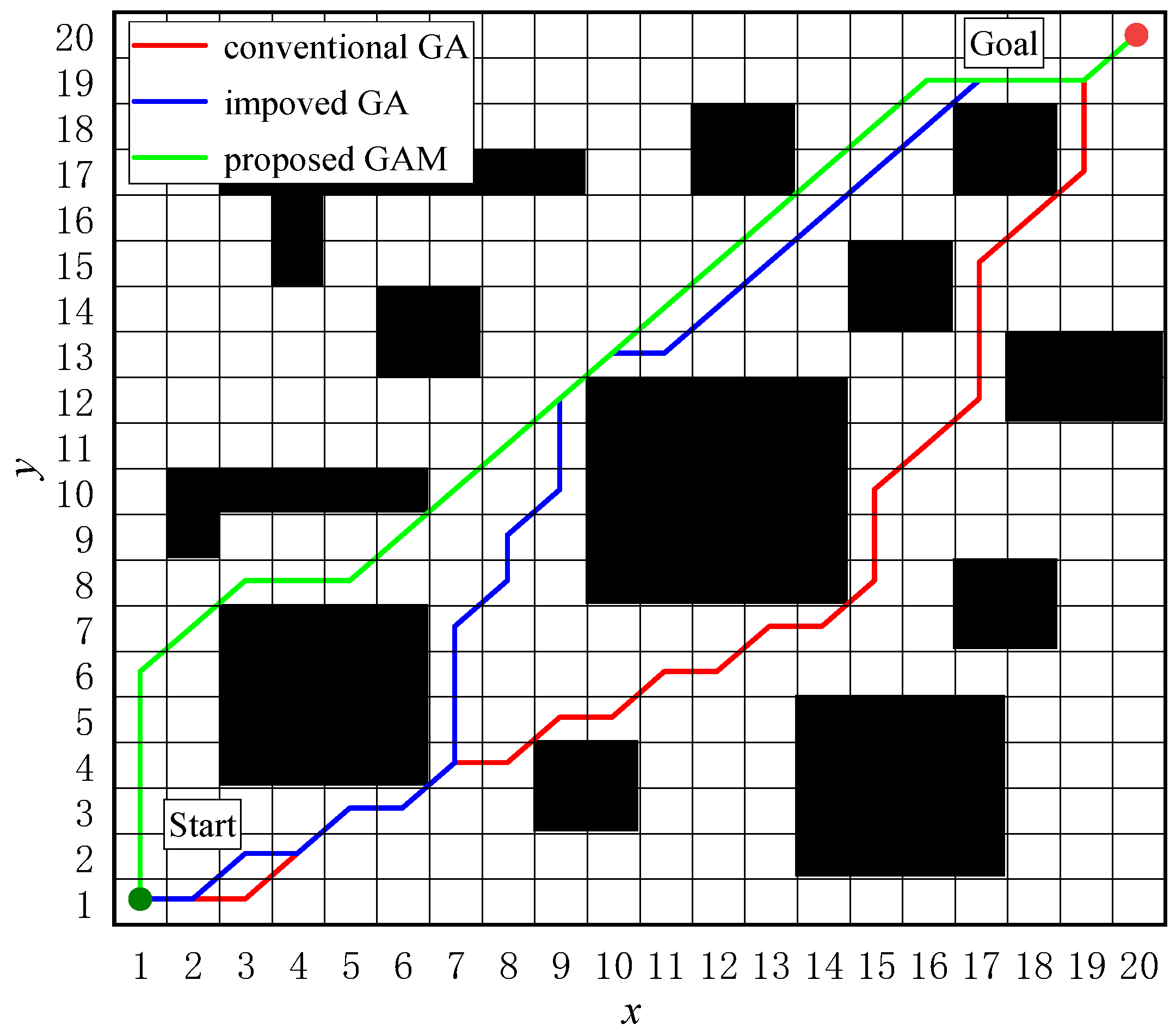
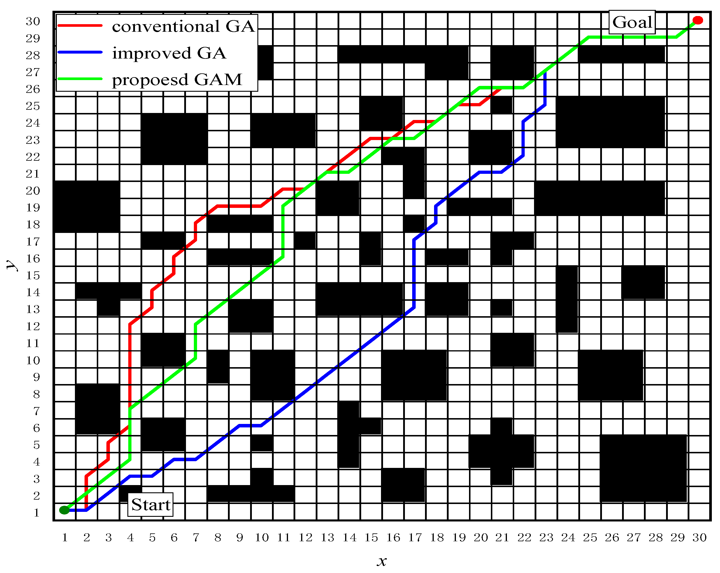
This paper conducted a comparative study of the GAM algorithm against both the traditional GA and an improved GA on 20 × 20 and 30 × 30 grid maps.

In the scenario of Figure 1, the underwater vehicle’s starting point is set at coordinates (1, 1), with target points at (a) (20, 20) and (b) (30, 30).

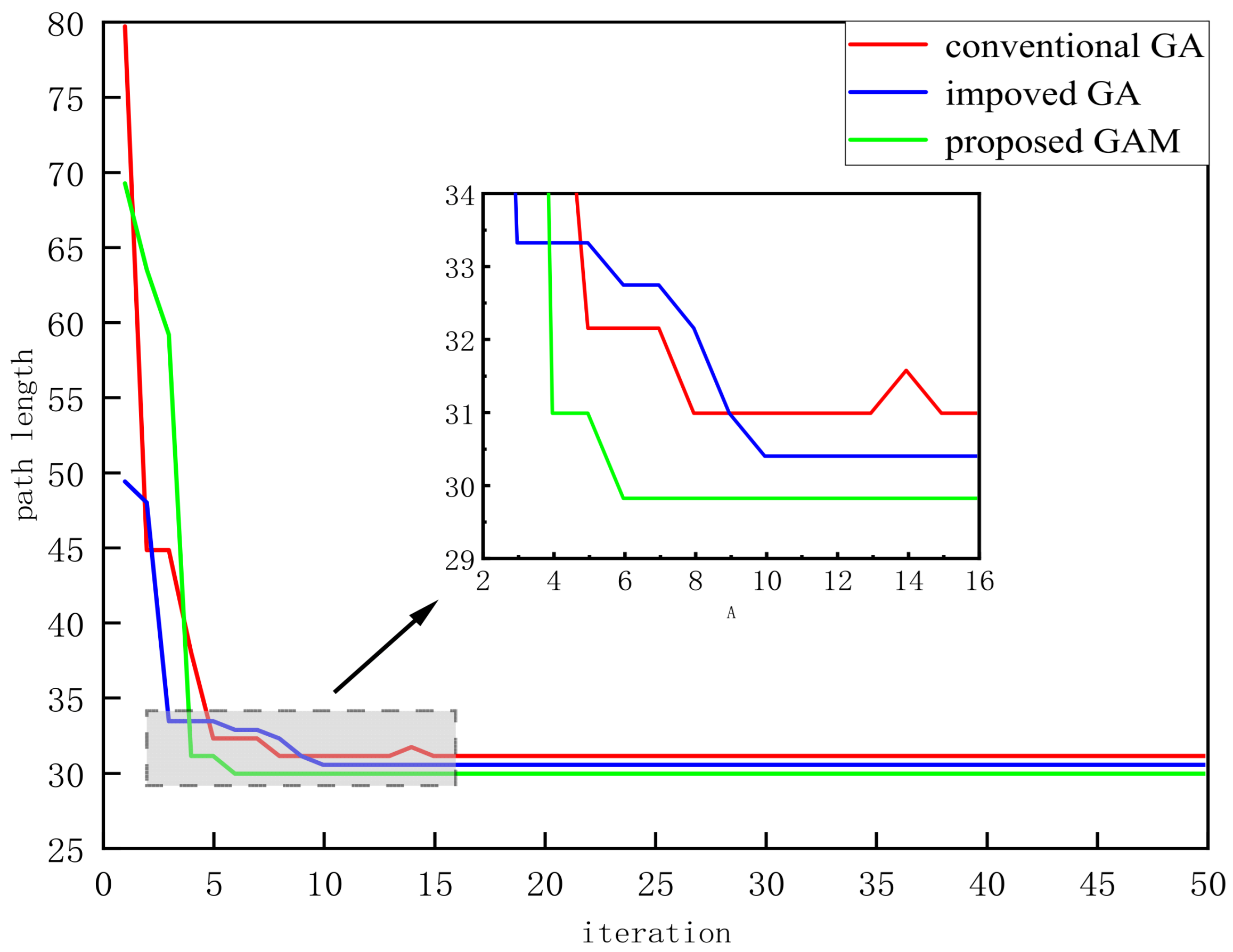
The GAM algorithm parameters are configured as follows: a population size of 50, a crossover probability of 0.8, a mutation probability of 0.2, and a maximum of 50 iterations. The calculation results are presented in Figure 2 and Figure 3. To eliminate the effects of randomness, each of the three algorithms was executed for 10 independent trials. The experimental results are presented in

Table 1. Path planning results, 20 × 20.

Parameter	Conventional GA	Improved GA	Proposed GAM
Optimal path length (m)	29.80	29.80	29.80
Average path length (m)	30.44	30.27	29.92
Average iteration	28.0	13.3	11.6
Inflection points	14.8	14.1	6.4

and

Table 2. Path planning results, 30 × 30.

Parameter	Conventional GA	Improved GA	Proposed GAM
Optimal path length (m)	46.28	45.70	45.70
Average path length (m)	47.08	46.10	45.82
Average iteration	48.8	33.7	21.8
Inflection points	25	25	16.9

below.

The simulation results indicate that the proposed migration operator enables the GAM algorithm to find the optimal solution faster while also demonstrating superior performance in reducing the inflection points. It is noted that the inflection point is determined by comparing the two movement directions of the adjacent three nodes.

As shown in Table 1, the proposed GAM algorithm demonstrates superior performance across all evaluated metrics. Specifically, it achieves reductions of 58.57% and 12.78% in the average number of iterations, and 56.76% and 54.6% in the average number of turns, compared to the traditional genetic algorithm and the improved algorithm, respectively.

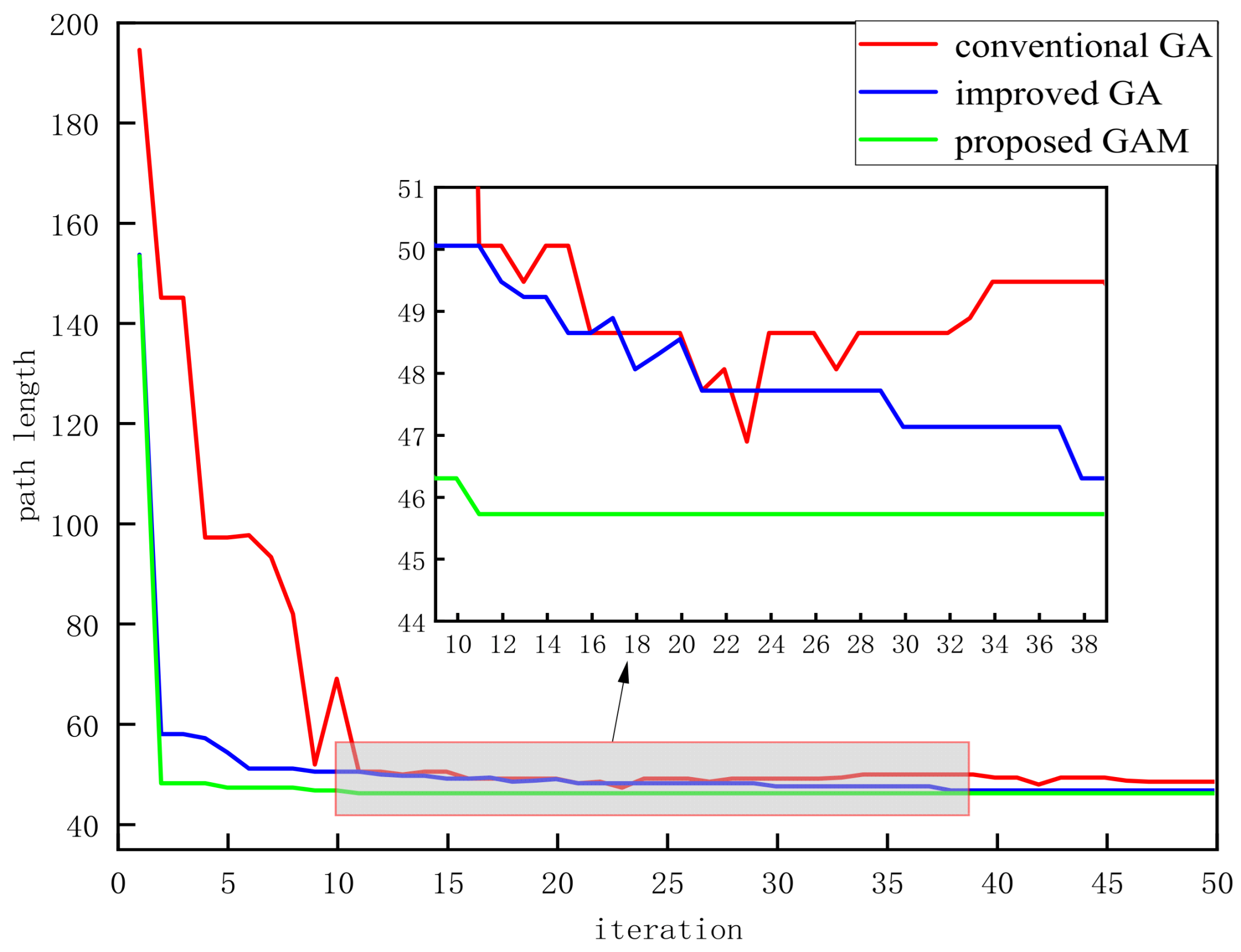
Figure 4 and Figure 5 illustrates that as map complexity grows, the required iterations and path turns increase, causing algorithm performance to diverge sharply. The traditional GA suffers from severe convergence issues, while the improved GA, though better, yields inadequate paths and slow convergence. The proposed GAM algorithm, however, demonstrates consistent robustness throughout.

As shown in Table 2, while the traditional genetic algorithm failed to find an optimal path, the proposed GAM algorithm achieved significant efficiency gains. It reduced the average iteration count by 55.33% compared to the traditional GA, and by 35.31% compared to the improved GA. Furthermore, GAM decreased the average number of turns by 32.4% relative to each of them. The simulation results confirm that the advantages of GAM become even more pronounced in complex maps with numerous obstacles.

3.2. GAM Combined with Flow Field

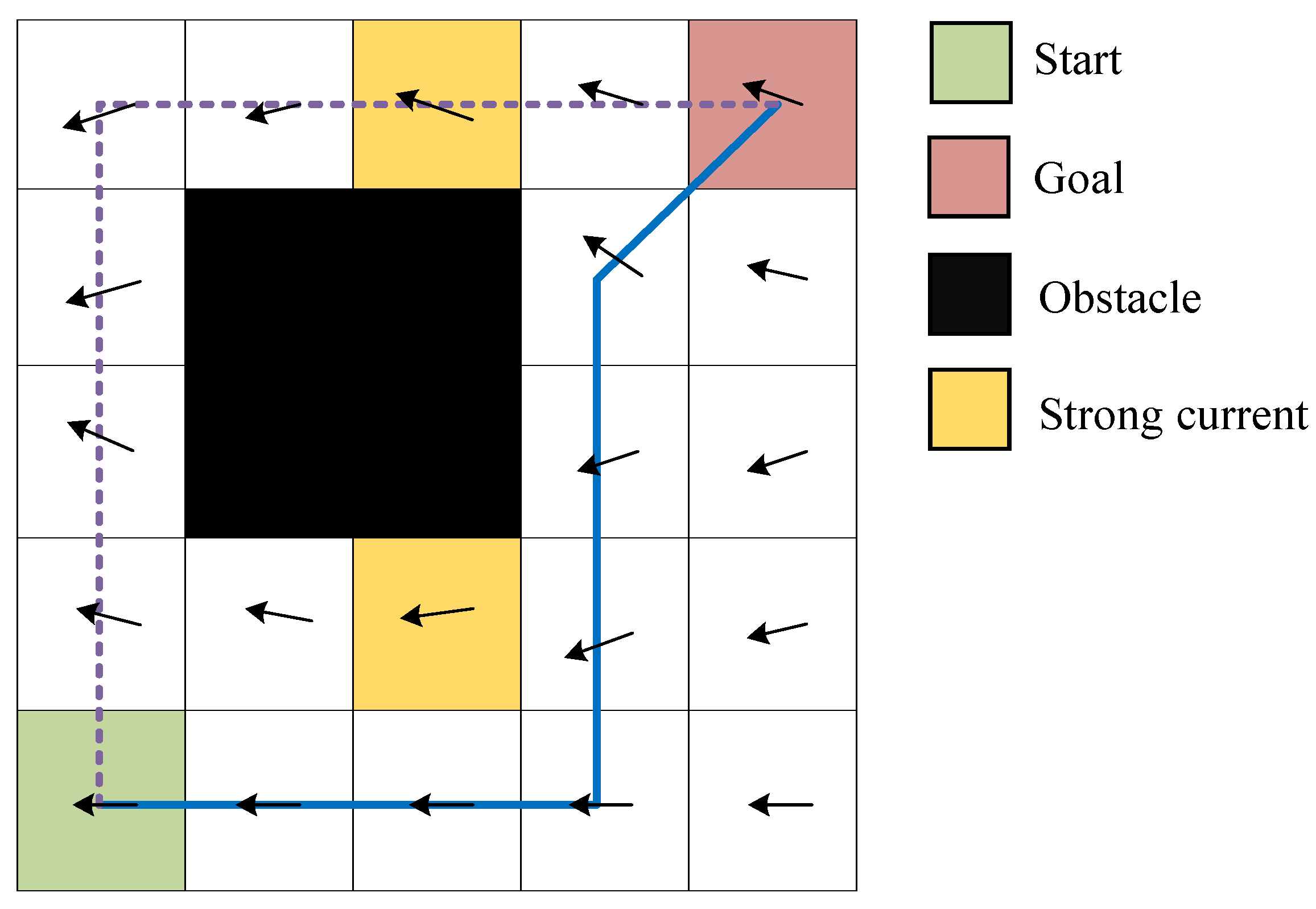
During path planning for an underwater vehicle, it is necessary to consider the impact of currents on the vehicle and avoid areas that are impassable due to strong currents where the velocities of currents are not less than the vehicle. Figure 6 shows an example of an infeasible path due to the strong currents. Both the purple dashed line and the blue solid line represent planned path candidates. However, the purple line is an infeasible path since it passes through a strong current area, although its length is seemingly shorter than the other planned path (blue line).

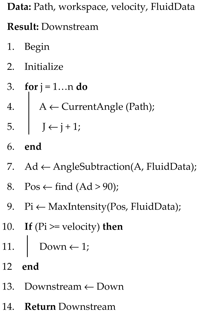
To avoid the infeasible path, a combinatorial path planning strategy is proposed, in which a module for determining the state of the underwater vehicle is incorporated into the GAM algorithm. The pseudocode of the algorithm is shown in Algorithm 2. After initialization, the path angle with the x-axis direction is calculated grid by grid using Formula (12). Subsequently, the flow field angle information is extracted by calculating the difference between the path angle and the corresponding flow field angle. When the angle difference is greater than or equal to the preset threshold, the strength information about the flow field at that location is queried. If the strength exceeds the maximum navigation speed of the underwater vehicle, the judgment coefficient is assigned as 1, indicating that an infeasible segment has been detected in the planned path. Thus, the algorithm will replan the path to avoid the strong current area.

In Algorithm 2, CurrentAngle(Path) is obtained by extracting the flow field angle at each node along the path from Fluent; MaxIntensity(Pos, FluidData) retrieves the flow velocity value at a given position from the Fluent-derived fluid data; AngleSubtraction(A, FluidData) calculates the angular difference between the current path angle θ (computed via the cosine theorem) and the local flow field angle.

Algorithm 2

$$\left\{\begin{array}{l}\theta =\arccos \left({\displaystyle \frac{b^2+c^2-a^2}{2\times b\times c}}\right)\\ a=\sqrt{{\left(y_{i+1}-y_i\right)}^2}\\ b=\sqrt{{\left(x_{i+1}-x_i\right)}^2}\\ c=\sqrt{{\left(x_{i+1}-x_i\right)}^2+{\left(y_{i+1}-y_i\right)}^2}\end{array}\right.$$

(12)

where $\theta$ is the angle between the path and x-axis.

The angle between the direction of movement and the direction of current is defined as follows:

$$\beta =\theta -\alpha$$

(13)

where $\alpha$ is the angle between the direction of the current and the positive direction of the x-axis calculated by CFD.

4. Simulations

To verify the proposed algorithm, a simulation is conducted. In this study, the working environment of an underwater vehicle around bridge piers is simulated. In practice, single-column piers and double-column piers are representative settings for bridge construction. Therefore, in this paper, single-target path planning for a single-column pier setting and multi-target path planning for a double-column pier setting are studied, respectively. In addition, two stream scenarios are investigated, including downstream sailing and upstream sailing. To verify the advantages of the proposed path planning strategy (i.e., GAM), two algorithms are selected to be compared, including a conventional GA and an improved GA [31]. In [31], a factor of path smoothness is added to the fitness function.

4.1. 2D Path Planning

4.1.1. 2D Single-Target Path Planning

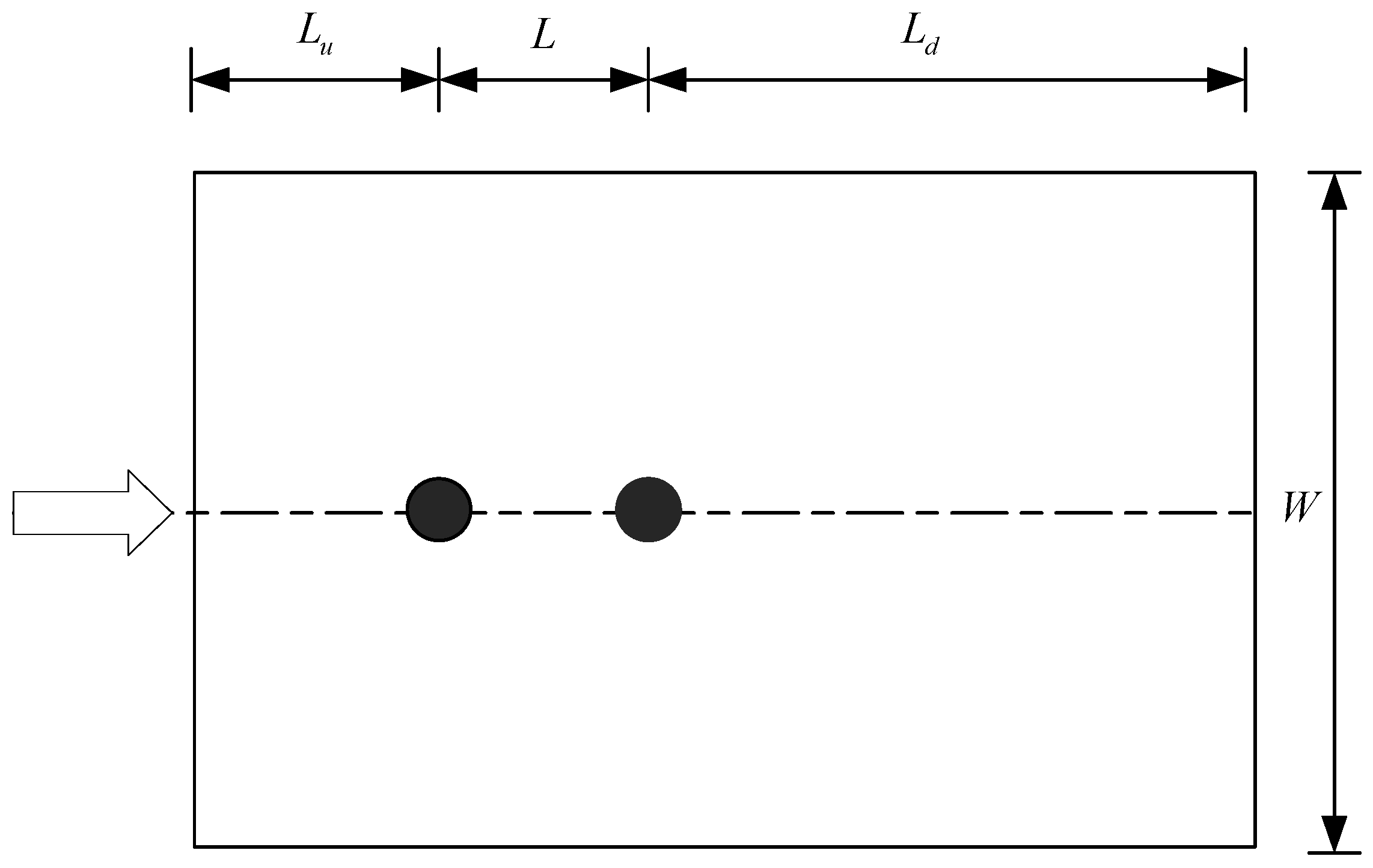
Firstly, the single-target path planning is studied using the proposed GAM. The computational domain for tandem-twin cylindrical piers is constructed as shown in Figure 7, where the arrow indicates the direction of the velocity inlet; L_u is the distance between the center of the left pier and the velocity inlet; L is the distance between the centers of the two piers; L_d is the distance between the center of the right pier and the outlet; and W is the width of the computational domain.

In the CFD numerical simulation, a structured grid is used and the turbulence model applied is the k-ω model. Local refinement is performed in the boundary layer area near the pier. Figure 8 shows the grid distribution. The number of cells is 317,226. The commercial solver ANSYS/FLUENT 2022R1 is employed for the numerical simulation. The finite volume method (FVM) is adopted to discretize the governing equations. The speed–pressure coupling equation is calculated by the Coupled algorithm. A second-order upwind scheme is adopted for momentum, turbulent kinetic energy, and turbulent dissipation rate. Underrelaxation factor is taken as the default value.

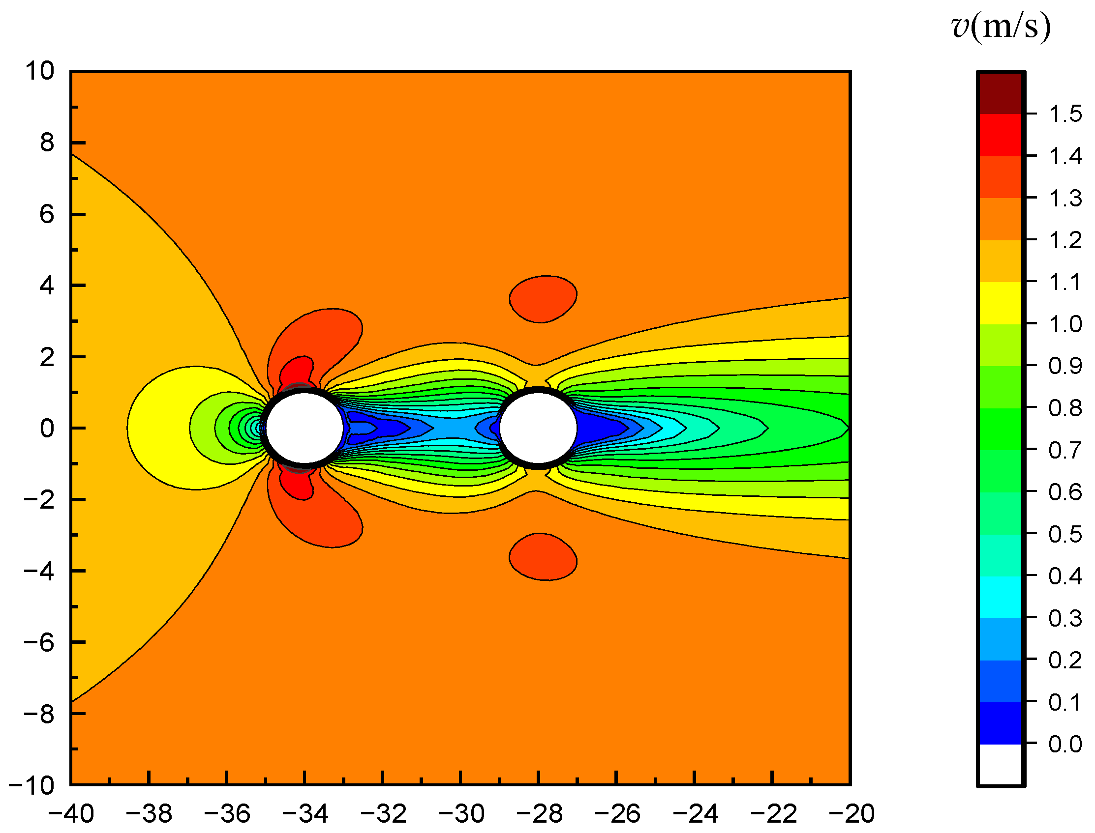
Figure 9 shows the flow field velocity distribution in the case of the diameter of pier D = 2 m, L_u = 15D, Ld = 46D, L = 3D, W = 30D, and an inlet velocity of 1.2 m/s. The corresponding Reynolds number can be calculated as Re = VD/ν = 2.39 × 10⁶, where V is the inlet velocity, while ν is the kinematic viscosity of fluid. From the calculation results, it can be concluded that the Reynolds number complies with the assumption of viscous flow. From the simulation results in Figure 9, it can be seen that there are symmetrically distributed high-flow zones around the pier. The maximum flow velocity occurs on both sides of the front pier. These results are consistent with experimental or numerical analyses of the flow around a cylinder in the literature.

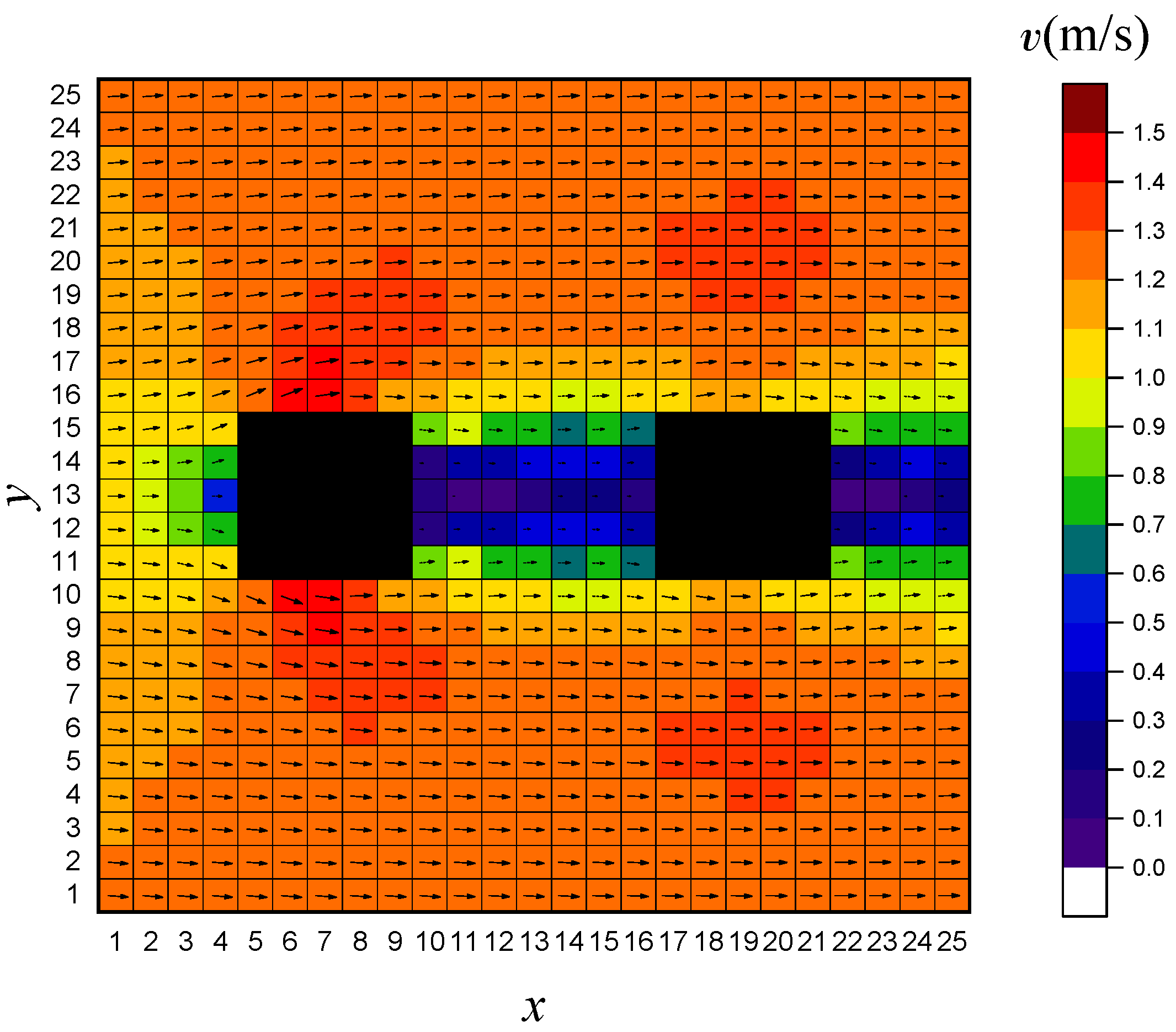
The obtained flow field is processed through grid discretization as follows. First, n × n data points are uniformly selected within the region of the flow field. Obstacle inflation is performed for the piers, shown as two black squares in Figure 10. Subsequently, m × m data points near the bridge pier are selected. The data from each point are assigned to the grid cells, ensuring a one-to-one relationship between the flow field data points and the grid cells in the grid map. The obtained grid map is shown in Figure 10, where different colors represent the intensity information for the flow field; the direction of the arrows represents the direction of the flow field velocity; their length corresponds to the magnitude of the flow field velocity.

Based on the grid map obtained from the CFD calculation, the path planning of an underwater vehicle is performed using the proposed GAM strategy. The underwater vehicle is viewed as a point mass. We assume that the planned path length remains within the operational range of the underwater vehicle and that the vehicle is able to rotate in place. We also assume that the influences of other factors such as surface vessels and electronic interference on the underwater vehicle are ignored. The maximum cruise speed of the underwater vehicle is set as v_max = 1.3 m/s. Figure 11 shows the planning results. Figure 11a gives the downstream path planning results, while Figure 11b gives the upstream results.

From the simulation results, it can be seen that for the downstream task, the paths planned by the three algorithms do not contain any infeasible regions. However, compared with the conventional GA and the improved GA [31], the number of inflection points decreases when using the proposed GA. Particularly in the presence of currents, the presence of inflection points implies extra energy costs for steering; therefore, fewer turns lead to lower energy consumption over paths of the same length. For the upstream task, due to the lack of consideration of the impact of the flow field on the underwater vehicle, infeasible segments in the planned paths occur when using both the conventional GA and the improved GA. If the underwater vehicle followed these planned paths, it would not reach the goal point successfully. Although the path planned by the proposed GAM increases the distance slightly, it guides the underwater vehicle to avoid strong current areas (surrounded by the dotted purple circle in Figure 11b) and reach the destination smoothly.

Table 3. Path planning results, downstream.

Parameter	Conventional GA	Improved GA	Proposed GAM
Optimal path length (m)	28.56	28.56	28.56
Average path length (m)	28.79	28.56	28.56
Average iteration	18.4	6	5.5
Inflection points	14	14.6	4.3

and

Table 4. Path planning results, upstream.

Parameter	Conventional GA	Improved GA	Proposed GAM
Optimal path length (m)	29.38	29.38	31.97
Average path length (m)	29.56	29.38	31.97
Average iteration	18.6	10.6	8.8
Inflection points	13.8	14.4	5.7

compare the three different algorithms in terms of the length of the optimal path, length of the average path, average iteration, and number of inflection points. Each algorithm runs ten times to obtain an average value. As can be seen, the proposed GAM performs excellently in all aspects, demonstrating superior path planning capabilities. The feasibility and practicality of the GAM in underwater vehicle path planning tasks based on flow field numerical simulation are validated.

4.1.2. 2D Multi-Target Path Planning

Compared with the single-column pier setting, the double-column pier setting is more commonly adopted in bridge construction in the light of its load bearing capacity and stability. The path planning for an underwater vehicle in the case of double-column piers might refer to multiply targets. Usually, the multi-target path planning problem is treated as a classic traveling salesman problem (TSP). In this paper, the proposed GAM is modified to solve this combinatorial optimization problem. The pseudo-code of TSP-GAM is described as Algorithm 3. First, the population is initialized by gathering information on each target point. Feasible solutions traversing each target point are obtained. Subsequently, the distance matrix is populated on the basis of the Euclidean distances between every pair of target points. Elite solutions are then extracted and excluded from subsequent operations to prevent the loss of high-quality solutions. Next, a migration operation is performed, in which segments of superior solutions are transferred to inferior solutions, allowing the latter to learn from the former, and their fitness values are thus improved. After selecting individuals for the remaining operations, a crossover operation is conducted to drive the population toward more optimal solutions. The feasible solutions are sorted according to their fitness values, with the top fifth classified as elite solutions and exempt from mutation. The remaining solutions undergo inversion mutation to generate new permutations and combinations, preventing the algorithm from converging to local optima. If the condition of maximum iteration is satisfied, the iteration stops and the optimal traversal sequence for the multiple target points is output.

Algorithm 3

It is noted that when the proposed TSP-GAM algorithm is used to solve the TSP problem, the obstacles between two target points are not taken into account. In such a case, the path traveled by the underwater vehicle is not a straight line between the two points. As a result, Euclidean distance cannot accurately represent the shortest path between the target points, and consequently the planned path might not be optimal. Therefore, when populating the distance matrix, the shortest path distance between each pair of target points in the grid map should be calculated. In this study, the GAM algorithm is employed and thus the combinatorial path planning algorithm TSP-GAM+GAM is proposed for the path planning of an underwater vehicle under complicated underwater environments. In detail, TSP-GAM is used to determine the traversal order of multiple target points, while GAM calculates feasible paths between the target points based on the traversal order.

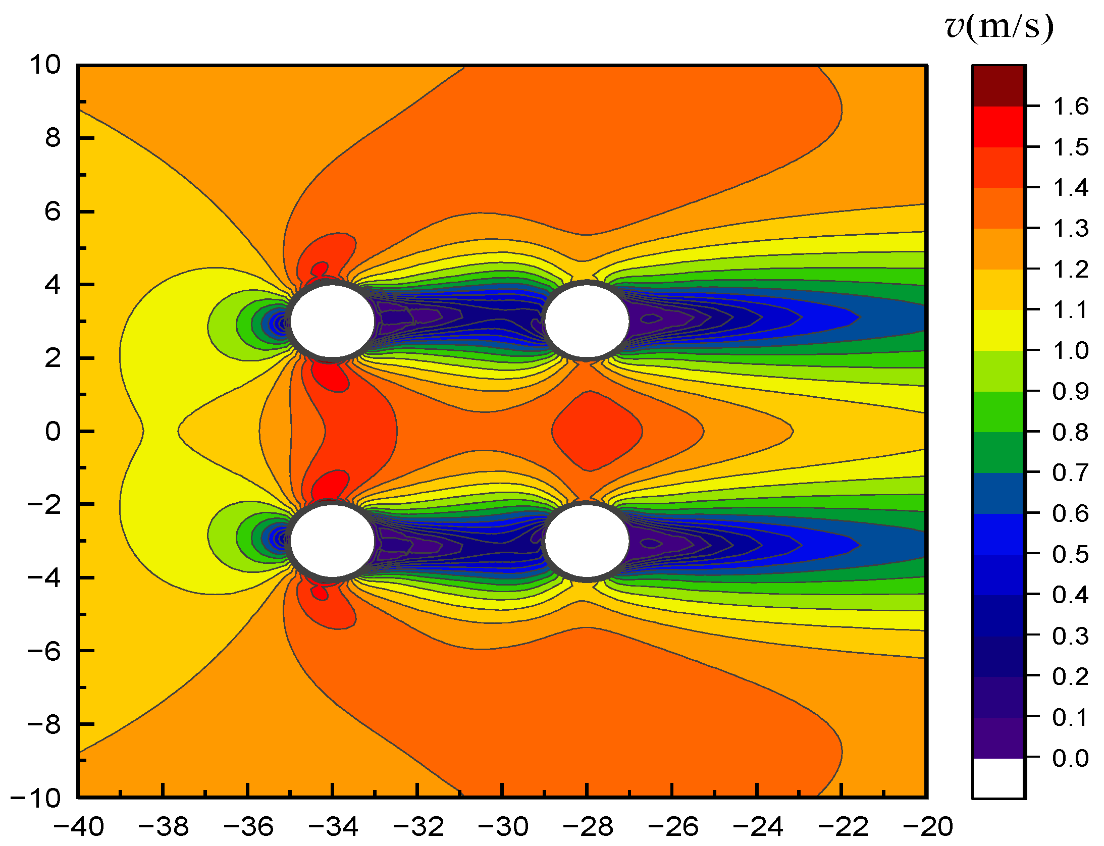
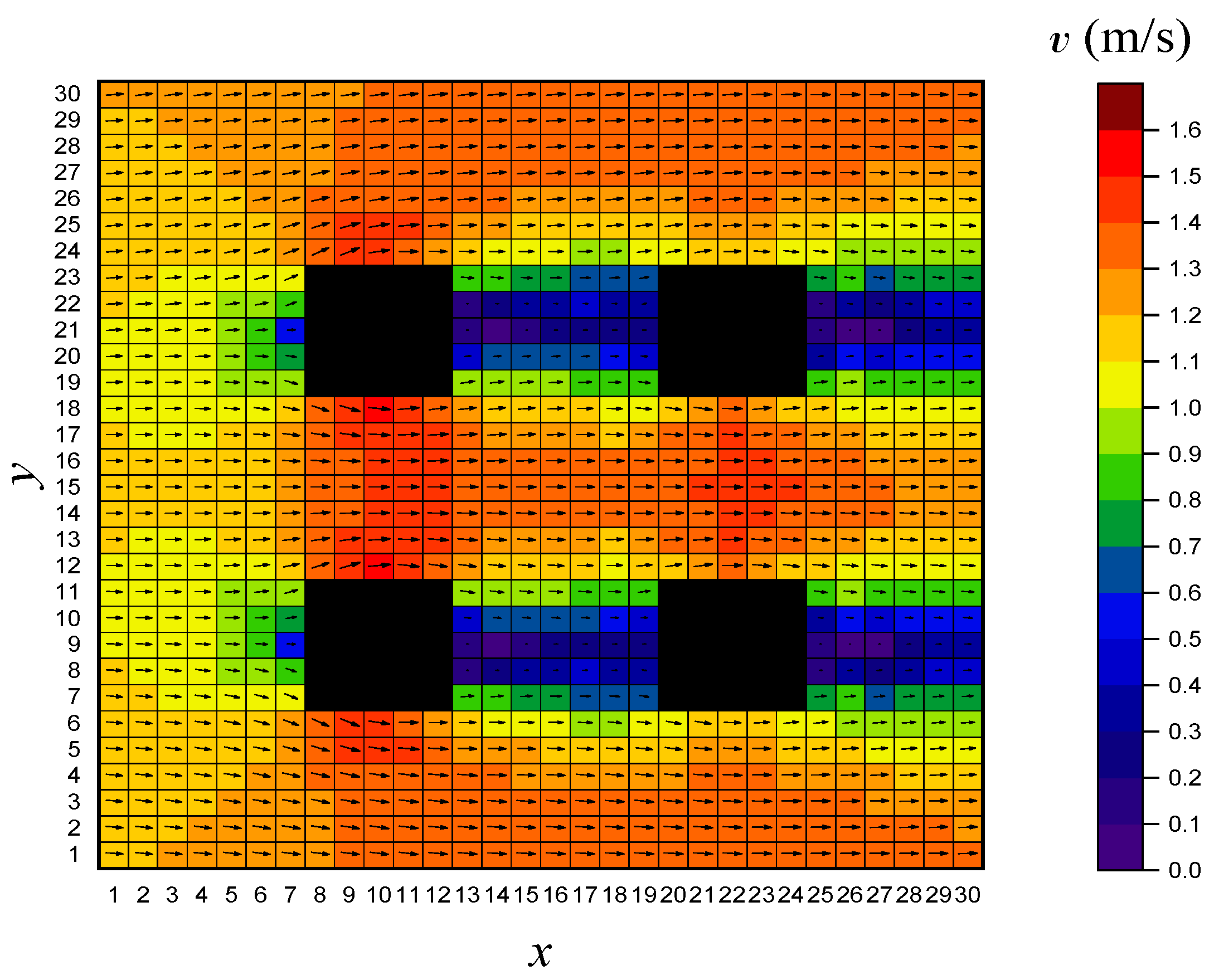
To incorporate the flow field information into the path planning, a CFD calculation is performed. Four piers are assumed to be the places where an underwater vehicle would pass through. We assume the inlet velocity is the same as in the single-target path planning, and the flow field velocity distribution is shown in Figure 12. As can be seen, the flow field becomes more complicated due to the interaction between lateral piers. The corresponding grid map is shown in Figure 13.

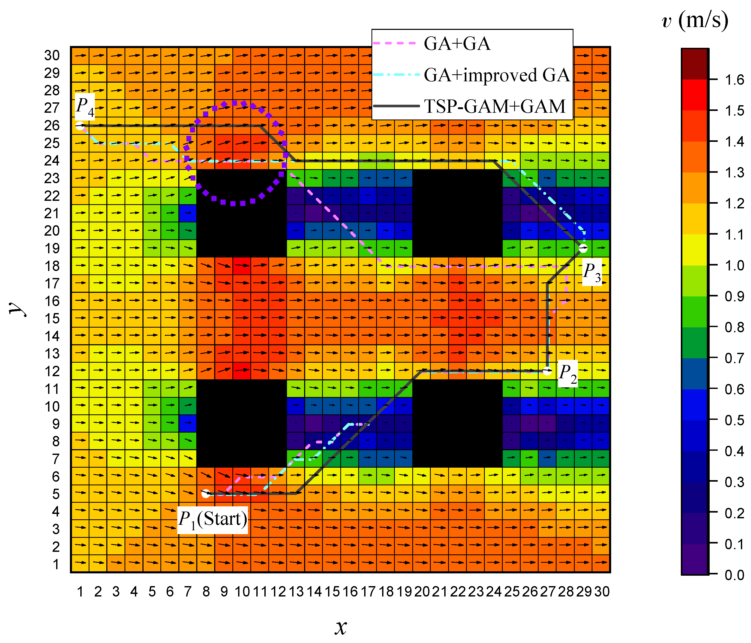
Based on the grid map of flow field, path planning is conducted using the algorithm TSP-GAM+GAM. The maximum cruise speed of the underwater vehicle is assumed to be v_max = 1.4 m/s. Four target points are set as P₁(8,5), P₂(27,12), P₃(29,19), P₄(1,26), respectively. P₁(8,5) is selected as the start point. To confirm the advantage of the proposed path planning strategy, i.e., TSP-GAM+GAM, two other planning strategies are compared. One uses the combination of GA+GA while the other adopts GA+improved GA [31]. Figure 14 shows the planning results and comparison. As can be recognized, under this setting of target points, the underwater vehicle should experience both downstream and upstream sailing. As can be seen, the traversal order of three algorithms is the same, i.e., P₁ ⟶ P₂ ⟶ P₃ ⟶ P₄. However, for the algorithms GA+GA and GA+improved GA [31], infeasible segments occur in the upstream areas when the underwater vehicle is moving from P₃ to P₄. In contrast, the proposed TSP-GAM+GAM algorithm effectively avoids the adverse strong current.

Table 5. Path planning results for four obstacles.

Parameter	GA+GA	GA+Improved GA	Proposed TSP-GAM+GAM
Traversal order	P1P2P3P4	the same	the same
Optimal path length (m)	61.46	60.63	60.63
Average path length (m)	61.58	61.09	61.05
Average iteration	21.4	16.7	11.7
Inflection points	17.3	15.4	8.6

compares the three path planning strategies in terms of traversal order of targets, the length of optimal path, the length of average path, the average iteration, and the number of inflection points. Each algorithm runs ten times to obtain an average value. Figure 15 shows the running results of an iteration. As can be seen from the comparison, obvious improvement has been achieved in the light of iteration and inflection points, which confirms the feasibility of the proposed strategy for multi-target path planning under complicated flow field.

4.2. 3D Single-Target Path Planning

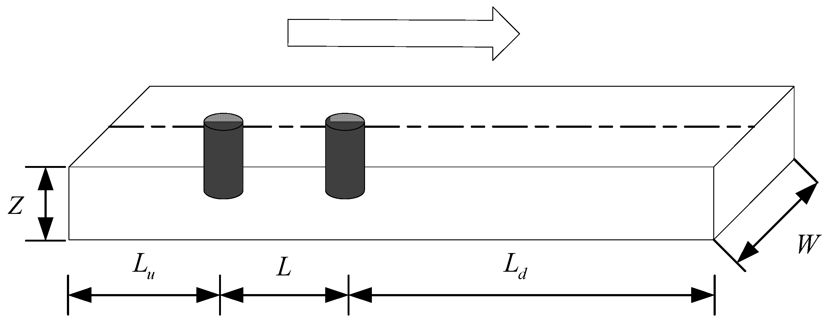
In a three-dimensional underwater environment, flow fields vary with depth, even at the same horizontal location, affecting the feasible space for path planning. The computational domain of the three-dimensional series double-cylindrical bridge piers is shown in Figure 16, where the arrow indicates the direction of the velocity inlet; Z is the height of the computational domain, and Z = 5D. In this study, the vertical flow velocity profile is set to resemble the inverse C-type. The velocity magnitude is symmetric about the center line.

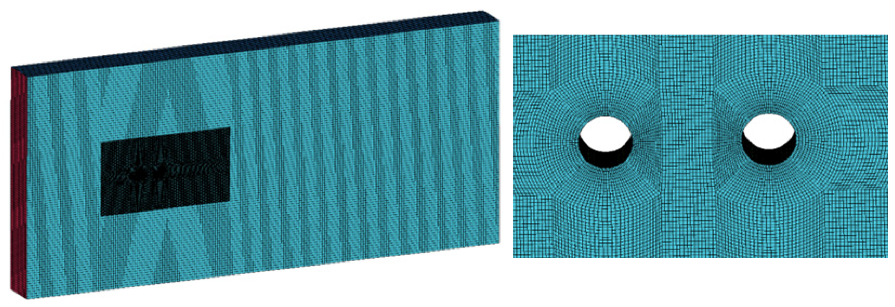
In the CFD numerical simulation, the structured grid is used and the turbulence model applied is the k-ω model. Local refinement is performed in the boundary layer area near the pier. Figure 17 shows the grid distribution.

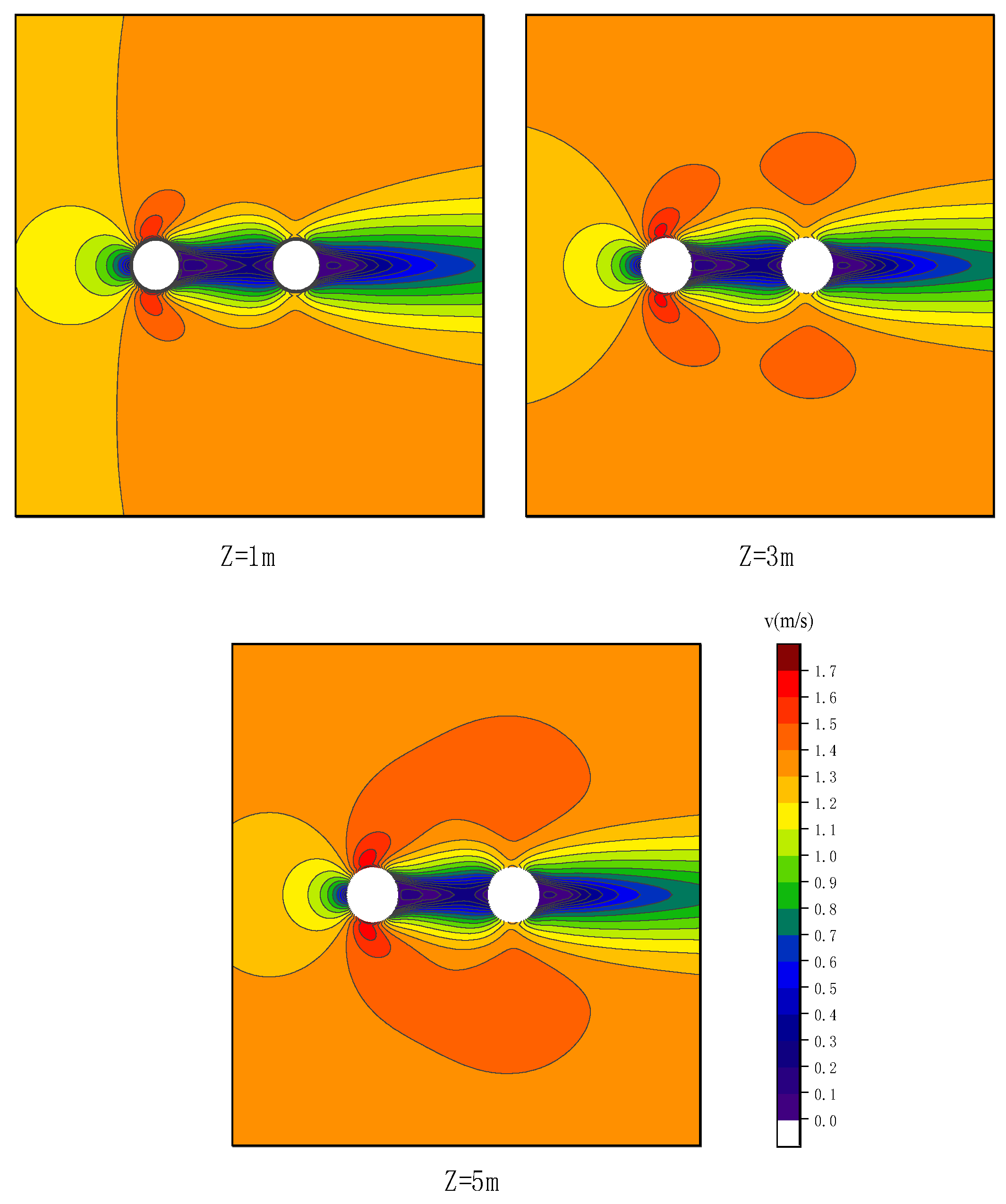
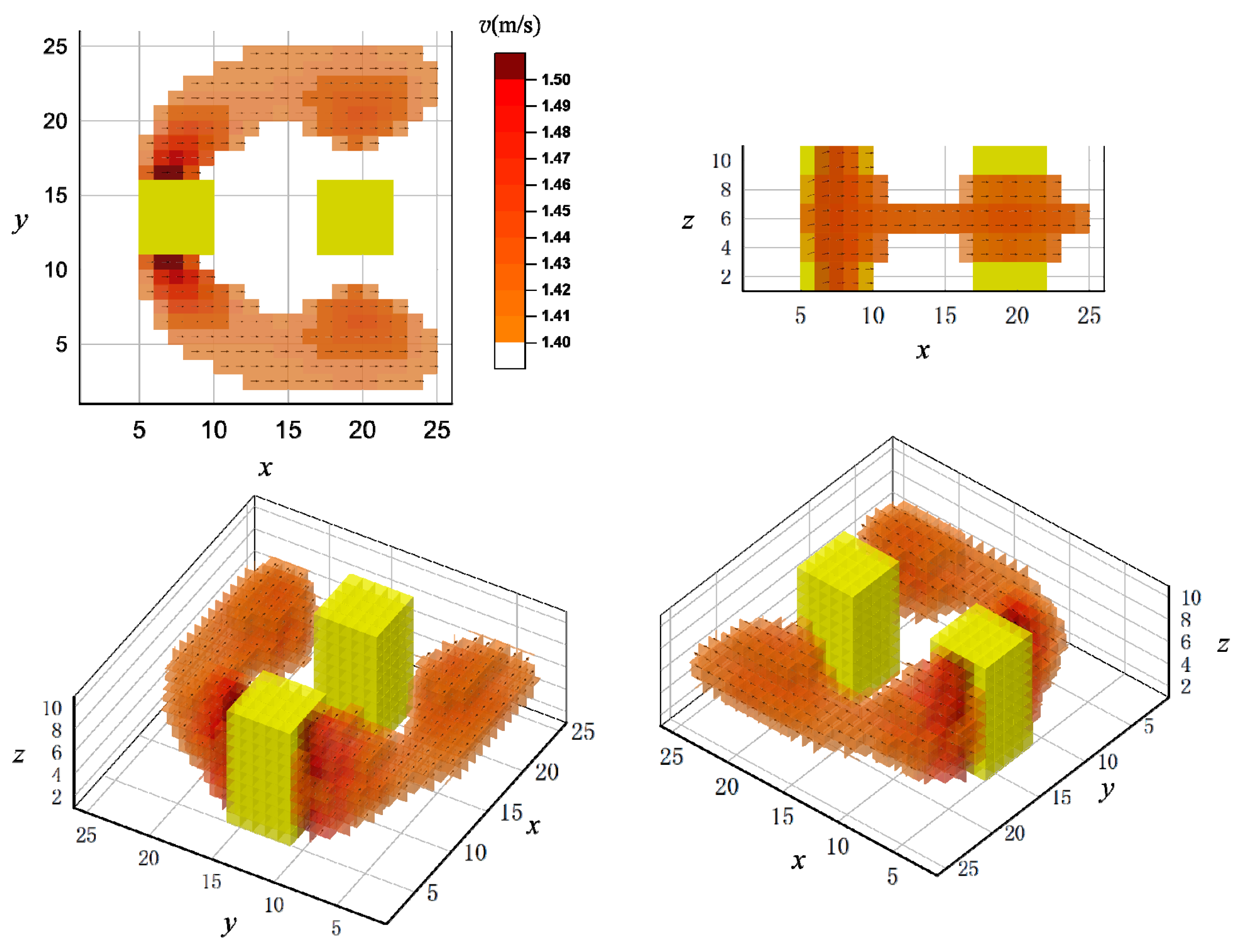
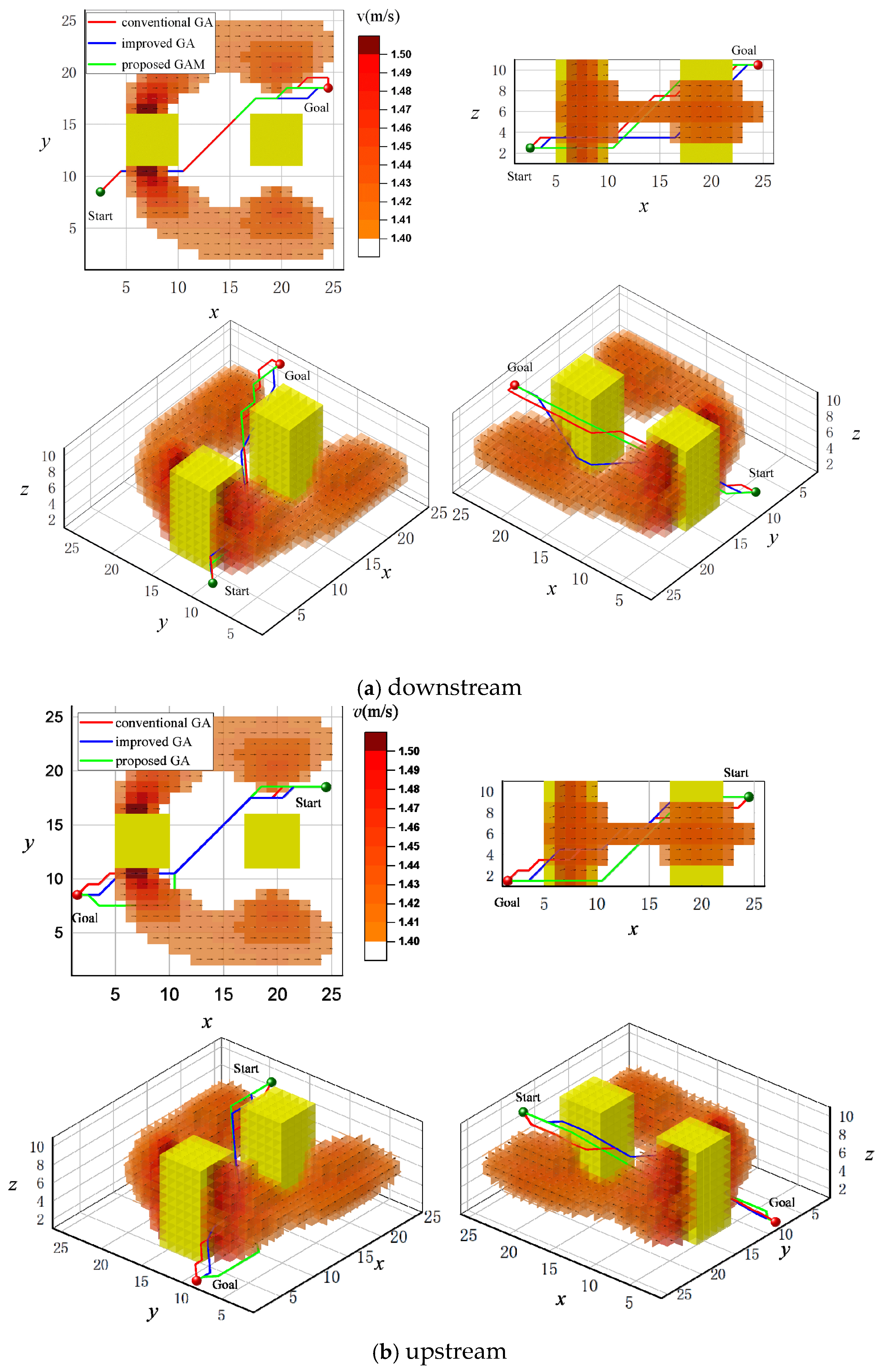
Velocity distribution maps of the flow field at different depths are shown in Figure 18. Figure 19 shows the grid map of the flow field, where yellow grid cells represent obstacles and the remaining cells represent flow fields. The color of each grid cell indicates the velocity magnitude, while the arrows within the cells denote the velocity direction.

The maximum speed of the underwater robot is set at 1.4 m/s. When the angle of the direction of the underwater vehicle movement is larger than 90 degrees from the flow field direction, the direction of movement is considered to be upstream. The parameters of the GAM algorithm, the traditional genetic algorithm, and the improved genetic algorithm are consistent. The population size is 50, and the maximum number of iterations is 50. Figure 20a gives the downstream path planning results, while Figure 20b gives the upstream results.

From the simulation results, it can be seen that the three algorithms generated paths that avoided infeasible regions. However, for the upstream task, both the conventional GA and the improved GA were unsuccessful due to their paths crossing strong current regions. In contrast, the proposed GAM algorithm successfully reached the goal by avoiding these regions.

Table 6. Path planning results: (a) downstream; (b) upstream.

Parameter	Conventional GA		Improved GA		Proposed GAM
	(a)	(b)	(a)	(b)	(a)	(b)
Optimal path length (m)	28.78	29.78	28.68	29.68	28.68	31.68
Average path length (m)	28.97	29.95	28.86	29.82	28.73	31.72
Average iteration	42.1	40.8	25	24.2	19.8	19.6
Inflection points	12.6	11.6	7.9	7.3	7.3	8

compares the three algorithms in terms of optimal path length, average path length, average iteration count, and number of inflection points. Each algorithm was run ten times to obtain average values. As shown, GAM performs excellently in all metrics for the downstream task. Although the conventional GA and improved GA produced shorter optimal and average path lengths than GAM, this comparison is only meaningful for the downstream case, as they failed to complete the upstream task.

5. Conclusions

In this paper, the path planning of an underwater vehicle is studied. The effect of currents on the underwater vehicle is taken into account by using CFD calculation to obtain the flow field data. This information is used to build a flow field database and then incorporated into the grid map for path planning. Based on the genetic algorithm, a hierarchical planning strategy is designed to prevent planned paths from being rendered non-viable due to the impact of strong current zones. Single- and multi-target point path planning are investigated. For multi-target point path planning, a combinatorial algorithm is proposed to solve the optimal traversal order of target points and plan a feasible path between target points. Through theoretical analysis and simulation, the feasibility and practicality of the GAM algorithm in path planning tasks based on numerical flow field simulations are verified. Compared with conventional GA and an improved GA, the number of average iterations and the number of average deflection points decrease to a considerable extent when using the proposed algorithm.

In our next work, a comparative analysis with other advanced algorithms will be conducted for a comprehensive evaluation of GAM. Moreover, the lack of tools for handling dynamically changing flow fields would limit the applicability of the CFD+GA approach. In future work, we plan to incorporate varying flow fields to enhance the applicability of the algorithm. In addition, to improve the feasibility of the path planning strategy, the dynamic model of an underwater vehicle will be considered.

References

1. Dijkstra, E.W. A note on two problems in connexion with graphs. Numer. Math. 1959, 1, 269–271. [Google Scholar] [CrossRef]
2. Guo, Q.; Zhang, Z.; Xu, Y. Path-planning of automated guided vehicle based on improved Dijkstra algorithm. In Proceedings of the 2017 29th Chinese control and decision conference (CCDC), Chongqing, China, 28–30 May 2017; IEEE: New York, NY, USA, 2017; pp. 7138–7143. [Google Scholar]
3. Gu, Y.; Ling, H.; Zhao, Y. Improved dijkstra’s algorithm based on optimized time window for autonomous maglev guided vehicle path planning. Appl. Res. Comput. 2025, 42, 2080–2085. [Google Scholar]
4. Zhang, H.; Cheng, Z. The method based on dijkstra of three dimensional path planning. In Proceedings of the 2020 Chinese Automation Congress (CAC), Shanghai, China, 6–8 November 2020; IEEE: New York, NY, USA, 2020; pp. 1698–1701. [Google Scholar]
5. Hart, P.E.; Nilsson, N.J.; Raphael, B. A formal basis for the heuristic determination of minimum cost paths. IEEE Trans. Syst. Sci. Cybern. 1968, 4, 100–107. [Google Scholar] [CrossRef]
6. Jiang, C.; Zhu, H.; Xie, Y.; Wang, H. Improved A* algorithm for path planning of mobile robot. Manuf. Technol. Mach. Tool 2024, 24, 33–36, 73. [Google Scholar] [CrossRef]
7. Song, R.; Liu, Y.; Bucknall, R. Smoothed A* algorithm for practical unmanned surface vehicle path planning. Appl. Ocean Res. 2019, 83, 9–20. [Google Scholar] [CrossRef]
8. Richter, J.; Kolvenbach, H.; Valsecchi, G.; Hutter, M. Multi-Objective global path planning for lunar exploration with a quadruped robot. In Proceedings of the 2024 International Conference on Space Robotics (iSpaRo), Luxembourg, 24–27 June 2024; IEEE: New York, NY, USA, 2024; pp. 48–55. [Google Scholar]
9. Zhang, L.; Lin, Z.; Wang, J.; He, B. Rapidly-exploring Random Trees multirobot map exploration under optimization framework. Robot. Auton. Syst. 2020, 131, 103565. [Google Scholar] [CrossRef]
10. Du, J.; Cai, C.; Zhang, P.; Tan, J. Path planning method of robot arm based on improved RRT* algorithm. In Proceedings of the 2022 5th International Conference on Robotics, Control and Automation Engineering (RCAE), Changchun, China, 28–30, October 2022; IEEE: New York, NY, USA, 2022; pp. 236–241. [Google Scholar]
11. Ruan, X.; Liu, S.; Zhu, X. Path planning algorithm of mobile robot based on AHMRRT. J. Beijing Univ. Technol. 2022, 48, 121–128. [Google Scholar]
12. Jiang, Q.; Man, Y.; Pu, X. Improved Path Planning Algorithm Based on RRT. In Proceedings of the 2024 2nd International Conference on Signal Processing and Intelligent Computing (SPIC), Guangzhou, China, 20–22 September 2024; IEEE: New York, NY, USA, 2024; Volume 10, pp. 463–466. [Google Scholar]
13. Li, Q.; Zhang, W.; Yin, Y.; Wang, Z.; Liu, G. An improved genetic algorithm of optimum path planning for mobile robots. In Proceedings of the Sixth International Conference on Intelligent Systems Design and Applications, Jinan, China, 16–18 October 2006; IEEE: New York, NY, USA, 2006; Volume 2, pp. 637–642. [Google Scholar]
14. Zhang, M.; Xin, S.; Fan, H. Path planning for mobile robot based on improved genetic algorithm. In Proceedings of the 4th International Conference on Mechatronics Technology and Intelligent Manufacturing (ICMTIM), Nanjing, China, 26–28 May 2023; IEEE: New York, NY, USA, 2023; pp. 382–386. [Google Scholar]
15. Abolhoseini, S.; Alesheikh, A.A. Dynamic routing with ant system and memory-based decision-making process. Environ. Syst. Decis. 2021, 41, 198–211. [Google Scholar] [CrossRef]
16. Zheng, J.; Sun, X.; Ji, Y.; Wu, J. Research on UAV path planning based on improved ACO algorithm. In Proceedings of the IEEE 11th Joint International Information Technology and Artificial Intelligence Conference (ITAIC), Chongqing, China, 4–6 December 2026; IEEE: New York, NY, USA, 2023; Volume 11, pp. 762–770. [Google Scholar]
17. Mo, H.; Li, Z. Bio-geography based differential evolution for robot path planning. In Proceedings of the 2012 IEEE International Conference on Information and Automation, Shenyang, China, 6–8 June 2012; IEEE: New York, NY, USA, 2012; pp. 1–6. [Google Scholar]
18. Liu, T. Research on Path Planning Application of Improved Biogeography-Based Optimization Algorithm. Master Thesis, Gulin University of Electronic Technology, Guilin, China, 2018. [Google Scholar]
19. Li, G.; Dong, W.; Wang, Y.; Zhu, D.; Liu, Q. Path planning of underwater vehicles based on improved whale optimization algorithm. In Proceedings of the 6th International Conference on Automation, Control and Robotics Engineering (CACRE), Hongkong, China, 15–17 July 2021; IEEE: New York, NY, USA, 2021; pp. 444–448. [Google Scholar]
20. Wu, Z.; Fu, X.; Li, S.; Zhuang, Y. Wheel mobile robot path planning based on improved whale optimization algorithm. Mach. Des. Res. 2024, 40, 167–175. [Google Scholar]
21. Madhusmita, P.; Bikramaditya, D.; Bibhuti Bhusan, P. Grey wolf optimization for global path planning of autonomous underwater vehicle. In Proceedings of the Third International Conference on Advanced Informatics for Computing Research (ICAICR’19), Shimla, India, 15–16 June 2019; pp. 1–6. [Google Scholar]
22. Sun, B.; Li, Y.; Zhang, W. Multipopulation grey wolf optimization for cooperative Multi-AUV path planning in complex underwater environments. IEEE Syst. J. 2025, 19, 837–847. [Google Scholar] [CrossRef]
23. Shin, G.H.; Yang, H. Deep reinforcement learning for integrated vessel path planning with safe anchorage allocation. Brodogradnja 2025, 76, 1–32. [Google Scholar] [CrossRef]
24. Xi, M.; Yang, J.; Wen, J.; Li, Z.; Lu, W.; Gao, X. An information-assisted deep reinforcement learning path planning scheme for dynamic and unknown underwater environment. IEEE Trans. Neural Netw. Learn. Syst. 2025, 36, 842–853. [Google Scholar] [CrossRef]
25. Wang, L.; Li, M.; Cai, J.; Liu, Z. Research on mobile robot path planning by using improved genetic algorithm. Mech. Sci. Technol. Aerosp. Eng. 2017, 36, 711–716. [Google Scholar]
26. Zhang, Y.; Zhang, J.; Guo, Z.; Zhang, L.; Shang, Y.; Chen, W. The study on dynamic modeling and path planning of a manta ray-inspired underwater glider. Brodogradnja 2025, 76, 1–35. [Google Scholar] [CrossRef]
27. Wang, H.; Wang, C.; Zhang, C.; Wu, Y.; Wang, D.; Xu FWang, H. Path planning of Saucer-type autonomous underwater glider based on AQPSO algorithm. Ship Eng. 2020, 42, 13–19+27. [Google Scholar]
28. Zhu, D.; Liu, Y.; Sun, B.; Liu, Q. Autonomous underwater vehicles path planning based on autonomous inspired Glasius bio-inspired neural network algorithm. Control Theory Appl. 2019, 36, 183–191. [Google Scholar]
29. Li, K.; Hu, Q.; Liu, J. Path planning of mobile robot based on improved multiobjective genetic algorithm. Wirel. Commun. Mob. Comput. 2021, 2021, 8836615. [Google Scholar] [CrossRef]
30. Yan, Z.; Zhao, Y.; Zhang, H. A method of UUV path planning with biased extension in ocean flows. In Proceedings of the 10th World Congress on Intelligent Control and Automation (WCICA 2012), Beijing, China, 6–8 July 2012; pp. 532–537. [Google Scholar]
31. Jiang, T.; Zhang, Z.; Cheng, Z.; Li, J.; Lu, J. Robot formation method with improved genetic algorithm and leader-follower. Comput. Eng. Appl. 2020, 56, 240–245. [Google Scholar] [CrossRef]
Figure 1. Grid maps: (a) 20 × 20 grid map; (b) 30 × 30 grid map.
Jmse 14 00074 g001
Figure 2. Planning path under 20 × 20 grid map.
Jmse 14 00074 g002
Figure 3. Convergence of different algorithms under 20 × 20 grid map.
Jmse 14 00074 g003
Figure 4. Planning path under 30 × 30 grid map.
Jmse 14 00074 g004
Figure 5. Convergence of different algorithms under 30 × 30 grid map.
Jmse 14 00074 g005
Figure 6. Feasible and infeasible paths in flow field.
Jmse 14 00074 g006
Figure 7. Computational domain.
Jmse 14 00074 g007
Figure 8. Grid generation.
Jmse 14 00074 g008
Figure 9. Flow field velocity distribution around tandem-twin cylindrical obstacles.
Jmse 14 00074 g009
Figure 10. Grid map of the flow field velocity.
Jmse 14 00074 g010
Figure 11. Path planning under flow field: (a) downstream; (b) upstream.
Jmse 14 00074 g011
Figure 12. The flow field velocity distribution around four cylindrical obstacles.
Jmse 14 00074 g012
Figure 13. The grid map of the flow field velocity for four obstacles.
Jmse 14 00074 g013
Figure 14. Path planning for four obstacles.
Jmse 14 00074 g014
Figure 15. Comparison of convergence between different optimization strategies.
Jmse 14 00074 g015
Figure 16. Computational domain under 3D flow field.
Jmse 14 00074 g016
Figure 17. Grid generation under 3D flow field.
Jmse 14 00074 g017
Figure 18. The flow field velocity distribution around tandem-twin cylindrical obstacles at different depths.
Jmse 14 00074 g018
Figure 19. Grid maps of the 3D flow field velocity.
Jmse 14 00074 g019
Figure 20. Path planning under 3D flow field: (a) downstream; (b) upstream.
Jmse 14 00074 g020