Article

DNN Predictive Model for Estimating the Metacetric Height of Small Fishing Vessels in South Korea at the Early Design Stages

1
Research Institute of Medium & Small Shipbuilding, Yeongam 58457, Republic of Korea
2
Division of Navigation Science, Mokpo National Maritime University, Mokpo 58628, Republic of Korea
*
Author to whom correspondence should be addressed.
J. Mar. Sci. Eng. 2025, 13(9), 1779; https://doi.org/10.3390/jmse13091779
Submission received: 9 August 2025 / Revised: 30 August 2025 / Accepted: 10 September 2025 / Published: 15 September 2025
(This article belongs to the Section Ocean Engineering)

Abstract

Small fishing vessels are highly susceptible to stability-related accidents due to their limited size and vulnerability to rough seas. Although both international and Korean regulations mandate minimum stability standards, accurately estimating the metacentric height (G0M) during the early design stage—when detailed drawings or hydrostatic data are unavailable—remains a challenge. To address this gap, this study proposes a deep neural network (DNN)-based predictive model that estimates the G0M of small vessels using only fundamental hull dimensions and derived design variables, such as length-to-breadth ratio and length multiplied by block coefficient. A dataset comprising 118 Korean fishing vessels and 359 different loading conditions was constructed using parameters typically available in the early stages of ship design. These inputs do not require detailed hydrostatic calculations or structural drawings, making the approach practical for conceptual design. The model demonstrates strong predictive accuracy across diverse hull configurations and loading cases. Unlike conventional methods that depend on finalized designs or roll-period measurements, the proposed model enables quick and approximate stability assessments at the preliminary design phase. It serves as an efficient design support tool to allow naval architects to assess regulatory compliance and overall stability early in the development process, contributing to safer and more effective vessel design practices. In addition, by enabling fast and data-driven assessment of vessel stability, the proposed model may also serve as a foundational tool in broader maritime digitalization efforts, including intelligent ship design and ship-port logistics automation.

1. Introduction

Small fishing vessels are significantly more prone to accidents compared to large commercial ships. This is primarily due to their limited size and structural vulnerability to harsh marine environments, including high waves and rough seas. In response to these risks, international maritime organizations have established and enforced stability regulations specifically targeting small fishing vessels [1]. Similarly, South Korea has introduced its own national regulations that mandate minimum stability standards for fishing vessels, particularly those exceeding 24 m in length [2].
To enhance maritime safety and prevent ship-related accidents, a wide range of modern technologies have been actively applied in recent years. Among these, artificial intelligence (AI)—particularly deep learning—has emerged as a transformative force in the maritime industry. Recent advances have shown promising results in various areas, including navigation and ship operation. For instance, machine learning has been employed to improve voyage efficiency by estimating fuel consumption [3]; deep learning has been used to extract ship dimensions from satellite imagery [4]; and deep reinforcement learning techniques have been applied to optimize route planning during navigation [5].
Beyond navigation, deep learning applications have also expanded into fields such as maritime safety assessment [6], ship emission prediction [7], optimal ship design [8], and wind turbine motion prediction [9], illustrating the growing integration of AI into multiple aspects of maritime technology.
In the field of ship stability assessment, a variety of technical approaches have been explored over the years. Traditionally, experimental methods and probabilistic calculations have been more commonly employed than artificial intelligence-based techniques. For example, some studies have attempted to estimate a ship’s metacentric height using real-time roll motion data [10]. Other works have focused on analyzing transverse stability by utilizing the GZ curve, either to predict the vessel’s roll period or to evaluate its righting characteristics [11,12,13]. Furthermore, research has also been conducted to examine the intrinsic relationships within the GZ curve itself as a key parameter for understanding a vessel’s stability behavior [14].
More recently, studies have emerged that estimate the metacentric height of fishing vessels based on loading conditions using structural drawings and hydrostatic data [15]. In addition, several works have proposed simplified stability indices by analyzing the GZ curve for fishing vessels and passenger ships [16,17,18]. These examples demonstrate growing research activity in the area of ship stability, particularly in efforts to estimate metacentric height or to develop practical evaluation tools based on simplified criteria. However, such studies have generally not extended into the use of artificial intelligence methodologies.
More recently, some recent efforts have begun to explore AI-based approaches, including deep neural networks (DNNs), for predicting ship stability characteristics. For instance, DNNs have been applied to estimate six degrees of freedom (6-DOF) ship motions under various sea conditions [19], and radial basis function (RBF) neural networks have been used to predict the metacentric height of ro-ro passenger ships in real-time [20].
A review of existing studies on metacentric height and ship stability estimation reveals several key limitations. While deep neural networks (DNNs) have been widely applied in the maritime and navigation sectors, their use in the specific area of stability prediction remains limited. Most previous studies have relied on roll period analysis or ship drawings to estimate stability parameters, rather than employing DNN techniques. Although some recent works have begun applying DNNs, they have largely focused on specific vessel types or operational conditions, rather than offering a generalizable model for various hull dimensions. Moreover, existing research has typically aimed at predicting stability during the ship’s operational phase, rather than during the early stages of design.
Considering these limitations, it would be highly beneficial to enable preliminary estimation of ship stability at the early design stage—when only basic design parameters such as length, breadth, and draft are available. This would allow designers to make quick assessments of whether a vessel is likely to meet regulatory requirements, even before detailed drawings or final structural decisions have been made.
Therefore, the primary aim of this study is to develop a DNN-based predictive model that can estimate the metacentric height (G0M) of small vessels during the early design phase. In addition to supporting naval architects during conceptual design, this approach may also be applicable to smart ship development and port logistics automation by facilitating early-stage integration of vessel performance data into maritime digital systems.
To support this objective, a comprehensive database of fishing vessels operating in South Korea was compiled and analyzed. The dataset includes a total of 118 vessels, comprising 359 distinct loading condition cases, each accompanied by detailed structural drawings and stability data. Based on this dataset, a DNN-based predictive model was developed to estimate the metacentric height (G0M). The proposed model utilizes basic ship design parameters—such as length, breadth, draft, and depth—which are typically available at the early design stage. The resulting model demonstrated promising predictive performance and was validated for accuracy and reliability, indicating its potential as a practical tool for early-stage stability assessment. The proposed model is intended to serve as a practical design support tool, allowing naval architects to assess approximate stability characteristics at the conceptual design stage. It offers an efficient method to evaluate the adequacy of preliminary design decisions, thereby supporting safer and more compliant vessel development from the outset.

2. Ship Stability Regulations

This chapter presents a comparative analysis between the domestic stability regulations applied to fishing vessels of 24 m or more in length and the stability-related provisions established by the International Maritime Organization (IMO). Through this comparison, the chapter aims to outline the key stability parameters that should be examined to enhance the stability performance of small fishing vessels operating under the domestic regulatory framework. Among the various stability parameters discussed in this chapter, the present study primarily focuses on G0M as the main subject of analysis.

2.1. The IMO Regulations on Small Fishing Vessels Stability

The 1977 Torremolinos International Convention provides fundamental guidelines for the stability performance of fishing vessels and applies to vessels with a length of 24 m or more. This regulation primarily assesses a vessel’s stability based on the GZ (righting lever) curve, and the key evaluation criteria are summarized in Table 1. According to the Convention, the required metacentric height (G0M) is set at 0.35 m, or 0.15 m for vessels exceeding 70 m in length or possessing significant upper structures. Additionally, the Convention specifies minimum required areas under the GZ curve in a detailed manner.
For smaller fishing vessels under 12 m in length, the International Maritime Organization (IMO) has issued a separate set of recommendations entitled “Safety Recommendations for Decked Fishing Vessels of Less than 12 m in Length and Undecked Fishing Vessels”, which was approved in 2010. These guidelines are intended to enhance the safety of small vessels operating at sea, in rivers, lakes, dams, or other bodies of water, and apply both to decked vessels under 12 m and to all undecked vessels.
In comparison with the Torremolinos Convention, which is mandatory for fishing vessels of 24 m and above, most of the recommended stability criteria for smaller vessels are substantially aligned with those applied to larger fishing vessels.

2.2. The Korea Domestic Regulations on Small Fishing Vessels Stability

A representative regulation governing the stability of domestic fishing vessels is the “Standards for Fishing Vessel Stability and Load Line Marks”. In the case of fishing vessels, different stability criteria are applied depending on the vessel’s size. Specifically, separate stability standards are established for vessels measuring 24 m or more but less than 40 m, and for those measuring 40 m or more in length.
For fishing vessels with a length of 24 m or more and less than 40 m, the required metacentric height (G0M) is specified based on the following formula.
G 0 M = 0.04 B + α B D β   °   m
where
B: Breadth of the fishing vessel (m)
D: Depth of the vessel in accordance with structural standards (m)
F: Freeboard, i.e., the vertical distance from the top of depth (D) to the corresponding load line (m)
α: Coefficient based on hull material—0.54 for steel or FRP vessels, 0.28 for wooden vessels
β: Parameter value defined in the fishing vessel stability regulations
In addition to the aforementioned G0M requirement, the regulation also specifies the minimum righting lever (GZ) value at the critical immersion angle based on the following formula. According to the regulation, the GZ at the critical immersion angle must be greater than the heeling moment induced by external forces divided by the vessel’s displacement weight. In other words, this provision is intended to ensure that small fishing vessels do not easily reach the critical immersion angle under external forces, thereby reducing the risk of flooding and enhancing overall safety.
G Z c > M c W
where
G Z c : Righting lever (in meters) at the critical immersion angle (or at 12 degrees if the immersion angle exceeds 12°)
M c : Heeling moment (in ton·meters) caused by external forces
W : Displacement of the vessel
For fishing vessels with a length of 40 m or more, detailed criteria are established for G0M and areas under the GZ curve, in a manner similar to international regulations. The specific requirements are summarized in the Table 2.

3. Ship Model Data

This chapter examines the detailed specifications and stability data of the vessels used in the development of the deep neural network (DNN) model for estimating the metacentric height (G0M). The dataset is based on fishing vessels operating in South Korea.

3.1. Vessel Specification Data

A total of 118 fishing vessels were used to develop the predictive model for estimating the metacentric height (G0M), as depicted in Figure 1. To enhance the model’s accuracy, multiple loading conditions—three to four different loading states such as Full Load Departure, Ground Departure, Full Load Arrival, and Partial Arrival—were considered for the same vessel. The research team developing the DNN model for stability maintains a database of 417 loading cases, among which 359 cases were utilized in the present study for the G0M estimation model.
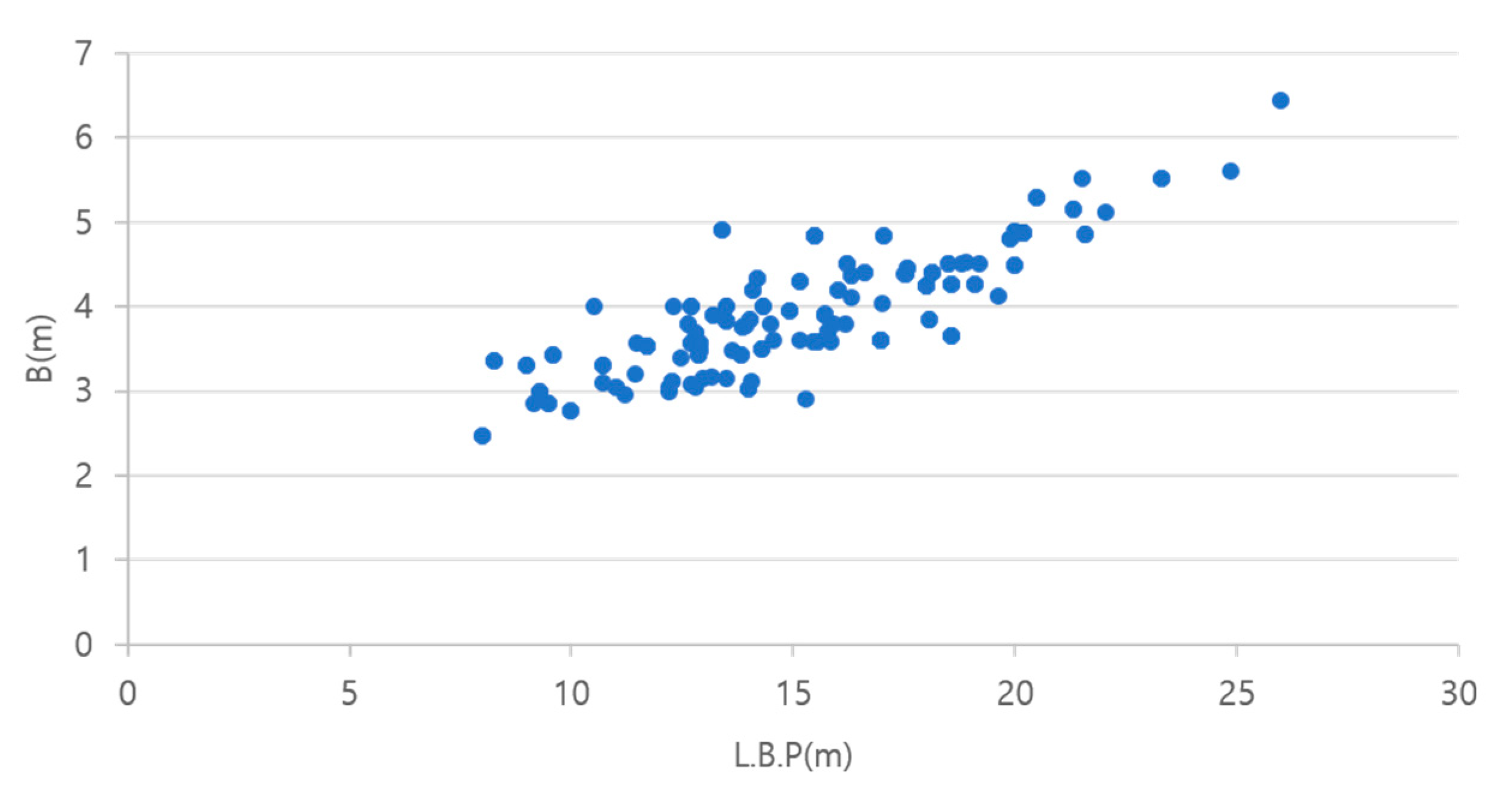
The distribution of vessel size, measured by gross tonnage, is shown in Figure 2. As shown, small vessels under 10 gross tons account for approximately 64% of the total dataset. The principal dimensions of the vessels range from 7 to 26 m in length and 2 to 6 m in breadth.

3.2. Ship Stability Data Distribution

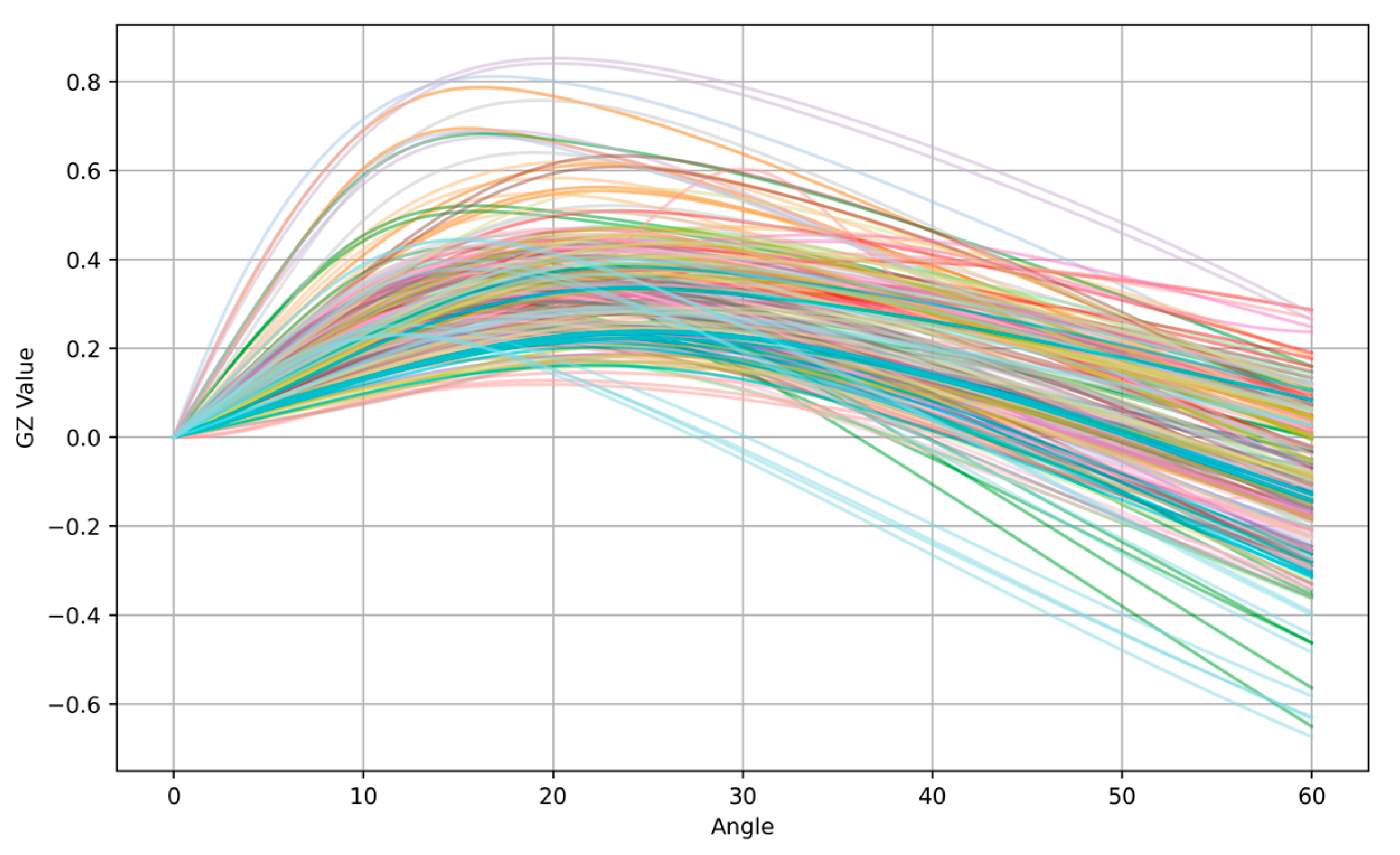
The overall distribution of stability performance for the vessels used in this study was analyzed in Figure 3. First, the GZ curves, a key indicator of stability, were plotted for all vessels. Compared to those of merchant ships, the GZ curves of fishing vessels exhibit certain differences. As shown in Figure 3, for most of the fishing vessels included in this study, the angle of vanishing stability—where the righting arm drops to zero—occurs between 30° and 40°. Additionally, the maximum GZ value typically occurs at an angle slightly above 20°. With the exception of some curves, it is rare for this value to exceed 25°.
These characteristics suggest that small fishing vessels may have weaker righting ability compared to merchant vessels at similar heel angles, highlighting the need for more careful consideration of their stability performance.
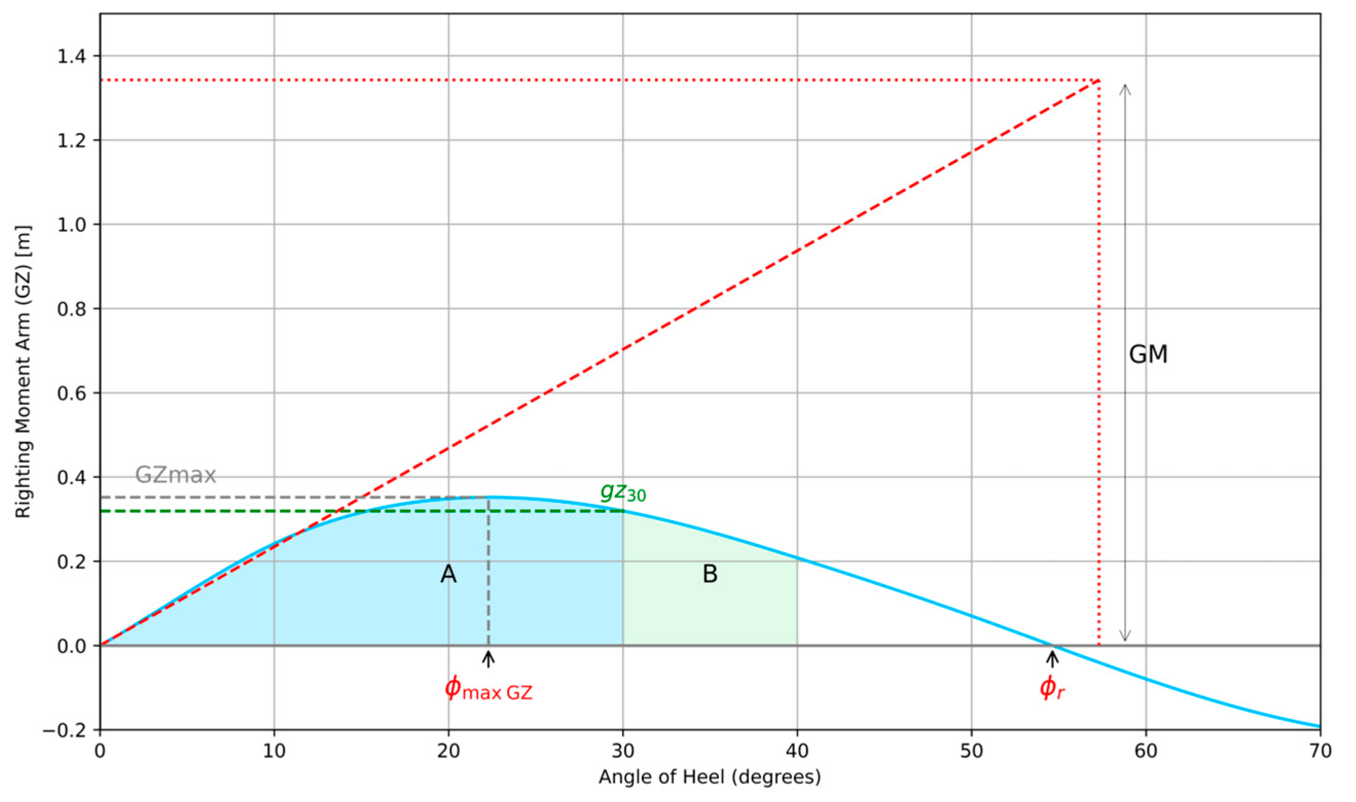
To more precisely quantify the stability performance of the fishing vessels represented by the plotted GZ curves, an average GZ curve was constructed and is shown in Figure 4. As presented, the maximum GZ value approaches 0.4 m, and the angle of vanishing stability is approximately 55 degrees. The angle at which the righting lever reaches its maximum is around 22 degrees, and the average metacentric height (G0M) is estimated to exceed 1.3 m. The DNN model developed in this study was trained using vessel data that exhibit these stability characteristics.

4. DNN Model for Estimating the Metacentric Height

This chapter provides a detailed overview of the deep neural network (DNN) model developed for estimating the metacentric height (G0M). It describes the model architecture, input and output variables, as well as the training and validation processes involved in the model development.

4.1. DNN Structure

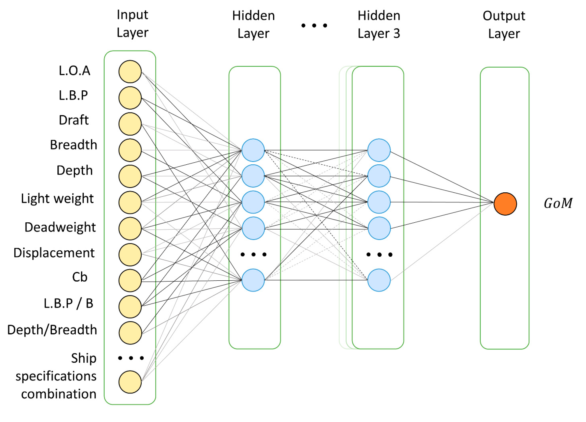
The G0M estimation model developed in this study consists of an input layer, three hidden layers, and a single output layer. The hidden layers comprise 128, 256, and 128 neurons, respectively, and are interleaved with Dropout layers to prevent overfitting, with the dropout rate set to 0.3. The architecture of the model is illustrated in Figure 5. As shown in the figure, the model produces a single output value representing the metacentric height (G0M), based on various ship specification parameters provided as input.
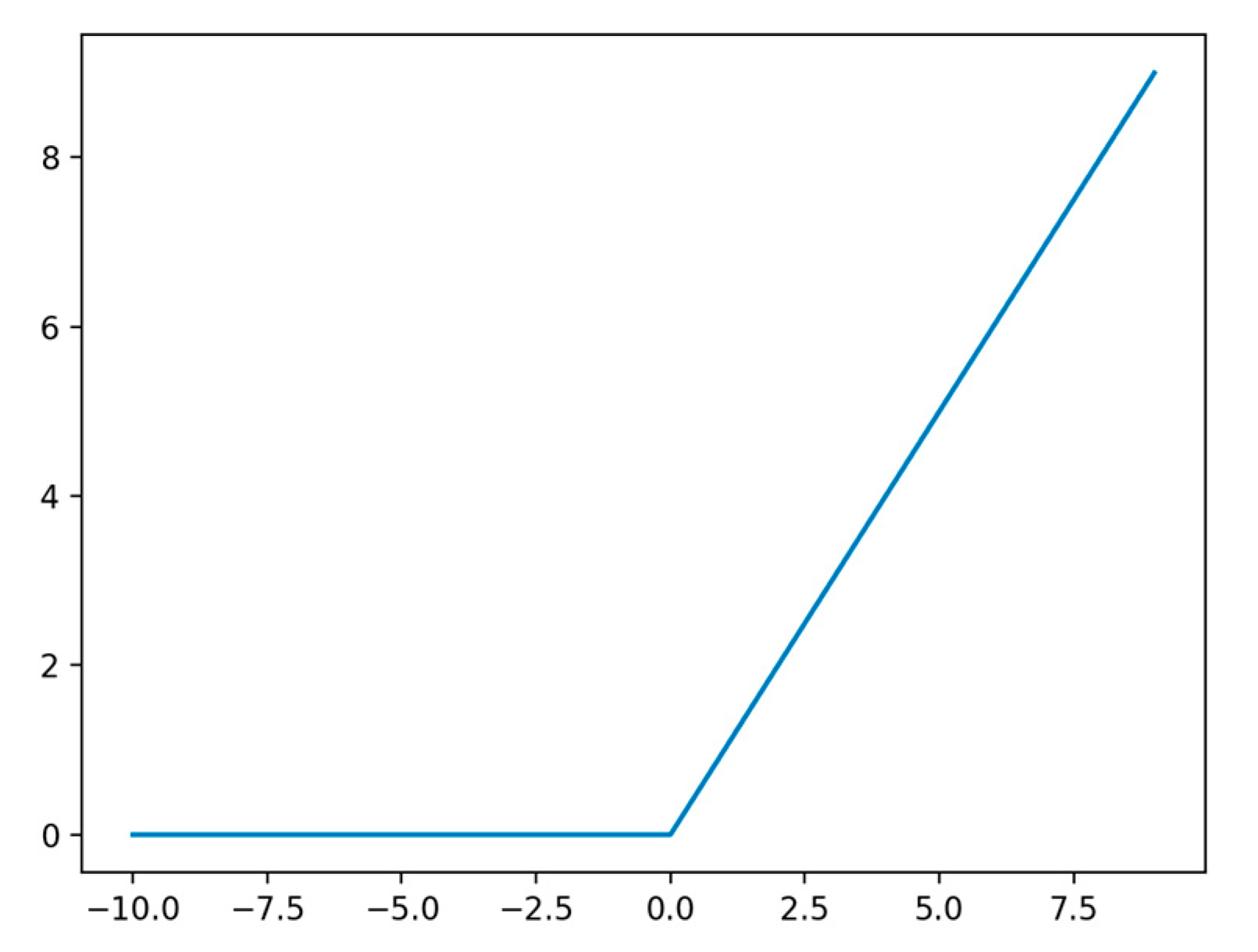
Each hidden layer utilizes the Rectified Linear Unit (ReLU) activation function, which introduces non-linearity and enables the network to learn complex relationships by allowing only positive values to pass through while setting negative values to zero. Specifically, the ReLU (Rectified Linear Unit) function outputs zero when the input is less than or equal to zero and returns the input value itself when it is greater than zero. The graph of the ReLU function is shown in Figure 6. The final output layer uses a linear activation function, which is a simple identity function that passes the input directly to the output without any transformation.
In this DNN architecture, the input features consist of various ship specification parameters. A total of 16 features is used, including basic geometric dimensions such as length, beam, and draft, as well as derived ratios such as length-to-beam (L/B) and beam-to-draft (B/d). The detailed list of input features is presented in Table 3. These parameters represent key design variables that can be defined during the early stages of ship design. In addition, since draft and displacement may vary depending on the loading condition—even for the same vessel—these variations were considered in the selection of input features to ensure that the model captures such dynamic changes effectively.

4.2. Data Preprocessing

The first step in model development involves preprocessing the input data obtained from ship specifications for use in the model. Preprocessing refers to the process of transforming raw data into a format suitable for model estimation. This step improves data quality and enhances the accuracy of the model.
The dataset used in this study did not contain inconsistent data or missing values; thus, data cleaning procedures were not necessary. Instead, the preprocessing primarily focused on the treatment of target values and input features.
The standardization of input features was performed using Equation (3), which represents the StandardScaler function provided by the Python package scikit-learn. This function adjusts the feature values so that the dataset has a mean of 0 and a standard deviation of 1. We applied this method because ship particulars, which cover a wide range of values and diverse parameters, required a scaling approach that preserves their distributional characteristics.
x i mean x stdev x
where
x i : original feature data
mean x : average of feature dataset
stdev x : standard deviation of feature dataset
To normalize the target value within a specific range, Equation (4) was used. This equation corresponds to the MinMaxScaler, which transforms each data point into a value between 0 and 1 by scaling it proportionally between the minimum and maximum values in the dataset. We applied this method because the target output, namely the ship’s metacentric height (G0M), has a relatively narrow value range and therefore required adjustment to a consistent [0, 1] interval.
y i min y max y min y
where
y i : original feature data
min y : minimum value of feature dataset
max y : maximum value of feature dataset
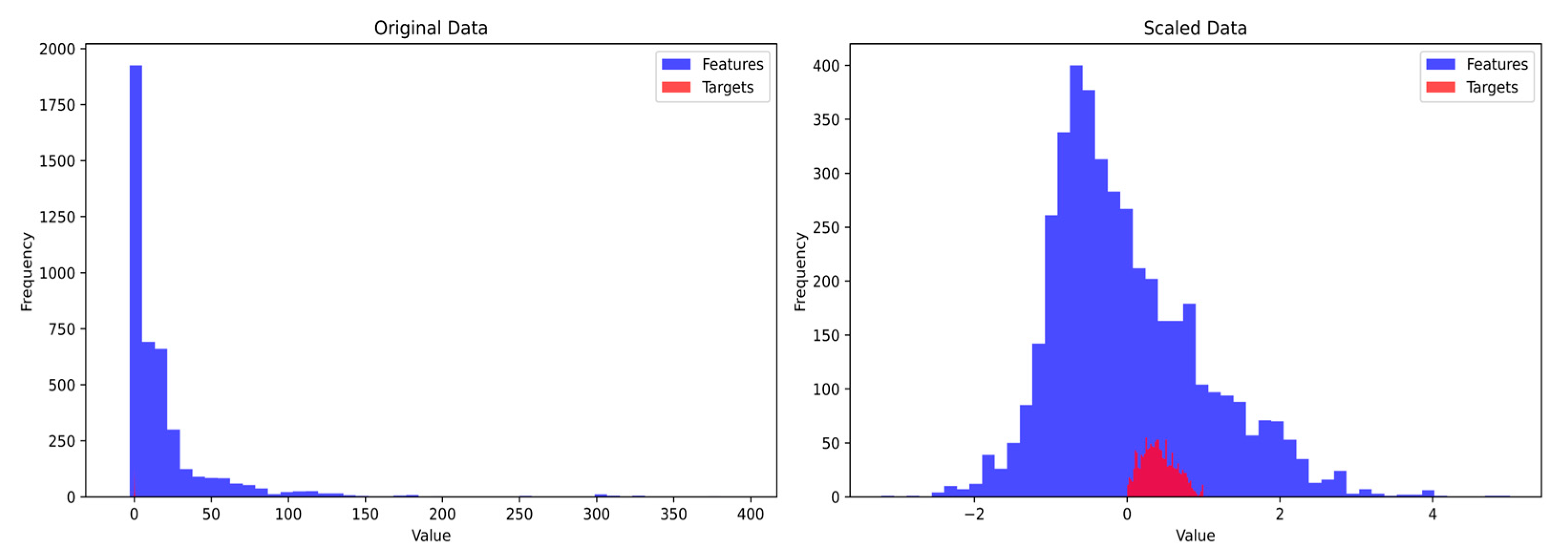
Figure 7 visually illustrate the state of the data before and after preprocessing. In the left of Figure 7, the blue feature values used for restoring stability are widely distributed, while the red target values appear in a very narrow range. After pre-processing, the right of Figure 7 shows that the feature values have been standardized to have a mean of 0 and a standard deviation of 1, while the target values have been normalized to lie within the range of 0 to 1. These results confirm that StandardScaler and MinMaxScaler were effectively applied to normalize the dataset within a consistent range.

4.3. Training Process

All model training and evaluation were conducted using Python 3.11.6. In this study, various combinations of hyperparameters were tested during the model training process. Among the resulting models, the configuration that exhibited the best performance on the validation dataset was selected as the final model. The specific hyperparameter settings used for the final model are summarized in Table 4.
The dataset was split in a ratio of 8:2 for training and testing, respectively. The network architecture consisted of three hidden layers with 128, 256, and 128 neurons, respectively. A dropout rate of 0.3 was applied to prevent overfitting.
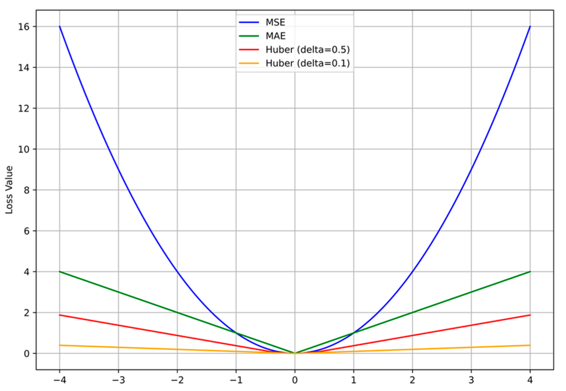
The loss function is a mathematical tool used to quantify the discrepancy between the model’s predicted outputs and the actual target values. In this study, the Huber loss function was selected for its robustness to outliers and its effectiveness in regression problems. This function integrates the characteristics of both mean squared error (MSE) and mean absolute error (MAE): it behaves quadratically for small errors to ensure stable convergence, and linearly for large errors to minimize the impact of outliers.
For optimization, the Adam algorithm was employed with a learning rate of 0.001, enabling efficient and adaptive updates of model parameters during training. The model was trained with a batch size of 32 for 1000 epochs to ensure convergence and performance stability.
The Huber loss function integrates the advantages of both MSE and MAE by behaving quadratically for small errors and linearly for large ones. To illustrate this characteristic, Figure 8 compares the shape of the Huber loss function with those of MSE and MAE. As shown in the figure, Huber loss transitions smoothly between the two, combining their strengths while mitigating their respective limitations.
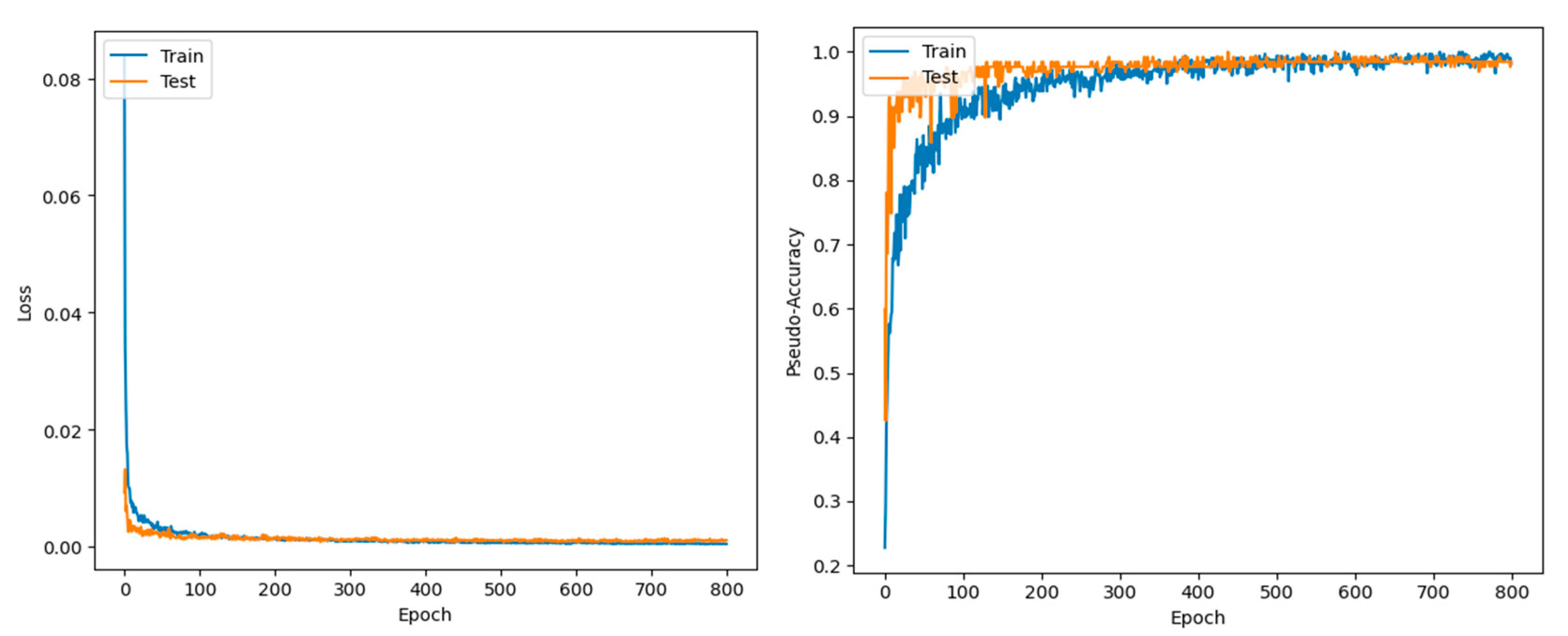
The training behavior of model is presented in Figure 5. The plot on the left shows the loss function values across epochs for both the training and test datasets. As observed, the loss remains consistently low throughout the training process, indicating rapid convergence and stable learning performance.
The plot on the right depicts a pseudo-accuracy curve, which evaluates model performance based on the proportion of predictions with an absolute error less than 0.1. The pseudo-accuracy rises sharply during the early epochs, surpassing 0.9 after approximately 100 epochs, and remains consistently high thereafter. These results demonstrate that the model generalizes well to unseen data and maintains a high level of predictive reliability. As shown in Figure 9, the training and test data demonstrate the learning performance well. In this study, the developed model was trained exclusively on the training data, and although Figure 5 presents the results for the test dataset, these results were not incorporated into the model and are provided for reference only.

4.4. Model Evaluation

In this study, the dataset was divided into training and test sets in an 80:20 ratio. In place of a separate validation set, model performance was assessed using the held-out 20% test set, which comprised 73 loading condition cases. This approach was considered appropriate given the practical focus of this study on early-stage vessel design support rather than model optimization. Upon completion of model training, the predictive performance was evaluated using the test dataset. Several statistical indicators were used to assess the model accuracy, including the coefficient of determination (R2), mean squared error (MSE), root mean squared error (RMSE), and mean absolute error (MAE). The mathematical expressions for these metrics are provided below. R 2 , MSE, RMSE, and MAE are presented in Equations (5)–(8), respectively.
R 2 = S S R S S T = 1 y i ^ y ¯ 2 y i y ¯ 2
where
S S R : Sum of Squares for Regression, representing the squared differences between the predicted values and the mean of the observed values;
S S T : Total Sum of Squares, representing the squared differences between the observed values and their mean;
y i : the actual observed value of the dependent variable;
y i ^ : the predicted value from the regression model;
y ¯ : the mean of the dependent variable;
M S E = 1 N i = 1 N y i y i ^ 2
R M S E = 1 N i = 1 N y i y i ^ 2
M A E = 1 N i = 1 N y i y i ^
where
y i : the actual (true) value at the i-th data point;
y i ^ : the estimated (predicted) value at the i-th data point;
N : the total number of data samples.
In estimating the model, the R 2 value is typically used to evaluate the goodness-of-fit of a predictive model. The other metrics—MSE, RMSE, and MAE—quantify prediction error. MSE represents the average of the squared differences between predicted and actual values, while RMSE is the square root of MSE, making the error more interpretable in the original scale. MAE indicates the average of the absolute differences between predictions and actual values.
The results of model validation are summarized in Table 5. The R2 value for the test dataset was 0.8701, indicating that the model explains a substantial portion of the variance in the target variable. The calculated values for MSE, RMSE, and MAE were 0.0577, 0.2402, and 0.1647, respectively. While the RMSE value suggests some degree of error—particularly when considering that most G0M values for small vessels are below 1—the overall predictive performance of the model can be considered satisfactory.
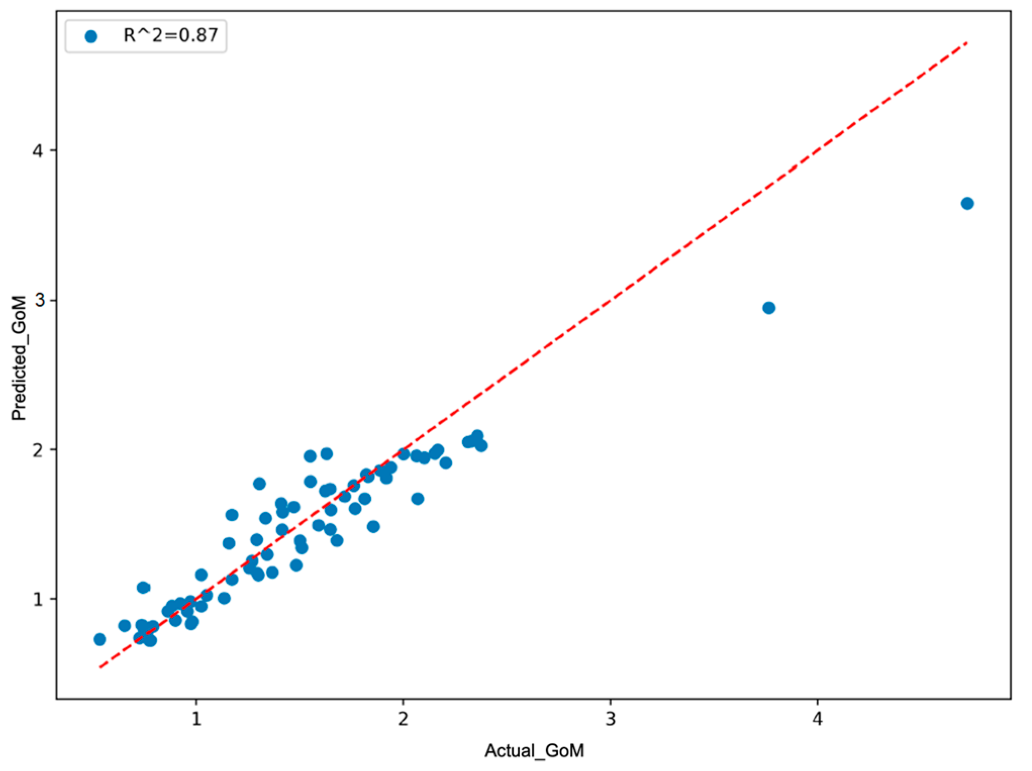
Figure 10 presents the scatter plot comparing the actual metacentric height (G0M) values with those predicted by the model on the test dataset. The red dashed line represents the ideal 1:1 correspondence line, where predicted values would exactly match the actual values. The distribution of the points along this line indicates the model’s overall accuracy. The coefficient of determination R2 = 0.87, as shown in the figure, suggests a high level of agreement between the predicted and actual values, confirming that the model captures the underlying trend of the data.
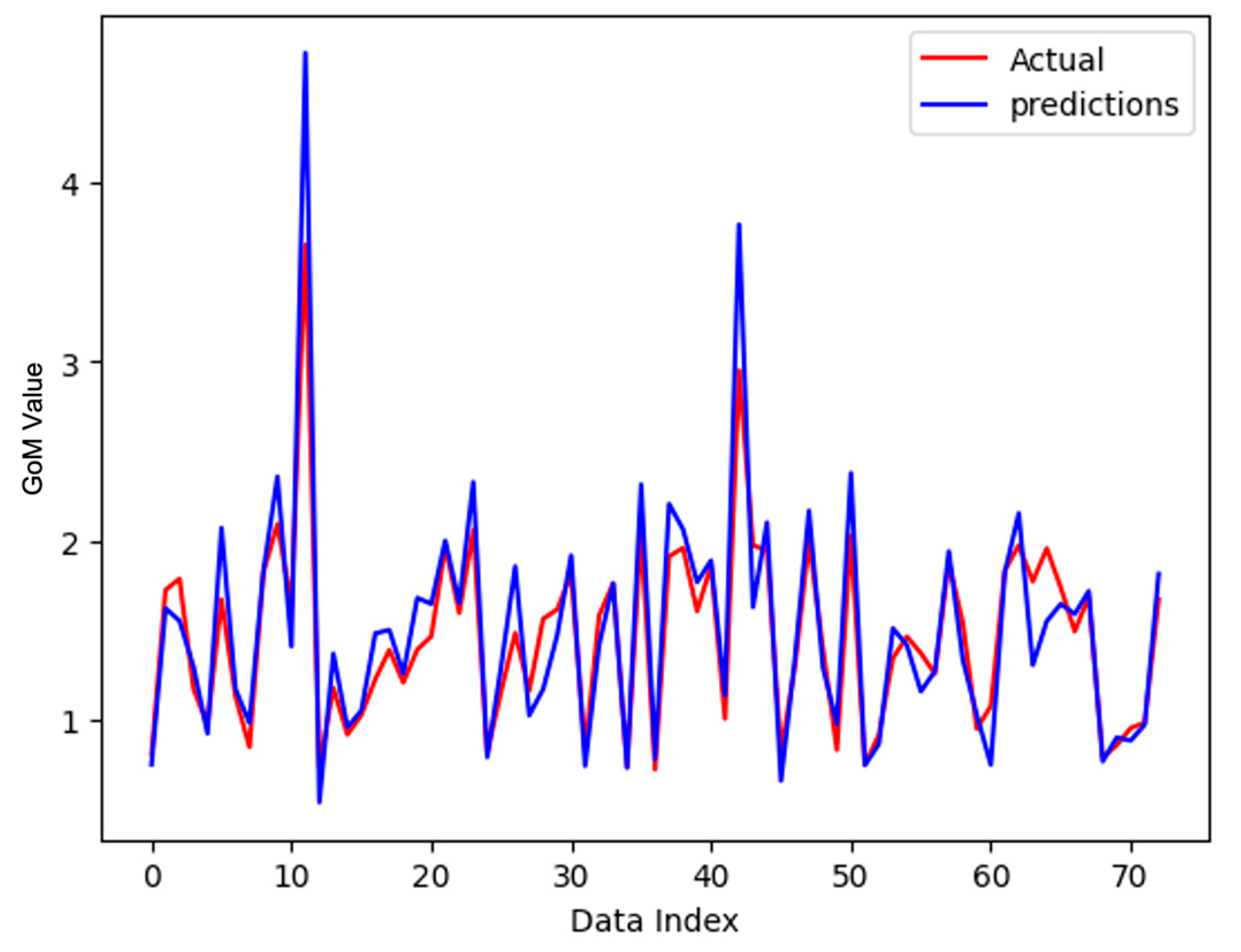
Figure 11 compares the predicted G0M values with the actual values for all 73 test cases. As shown, the model achieves good prediction accuracy across most data points. However, larger errors were observed in a few instances where the actual G0M exceeded 3, indicating potential challenges in handling outlier cases.
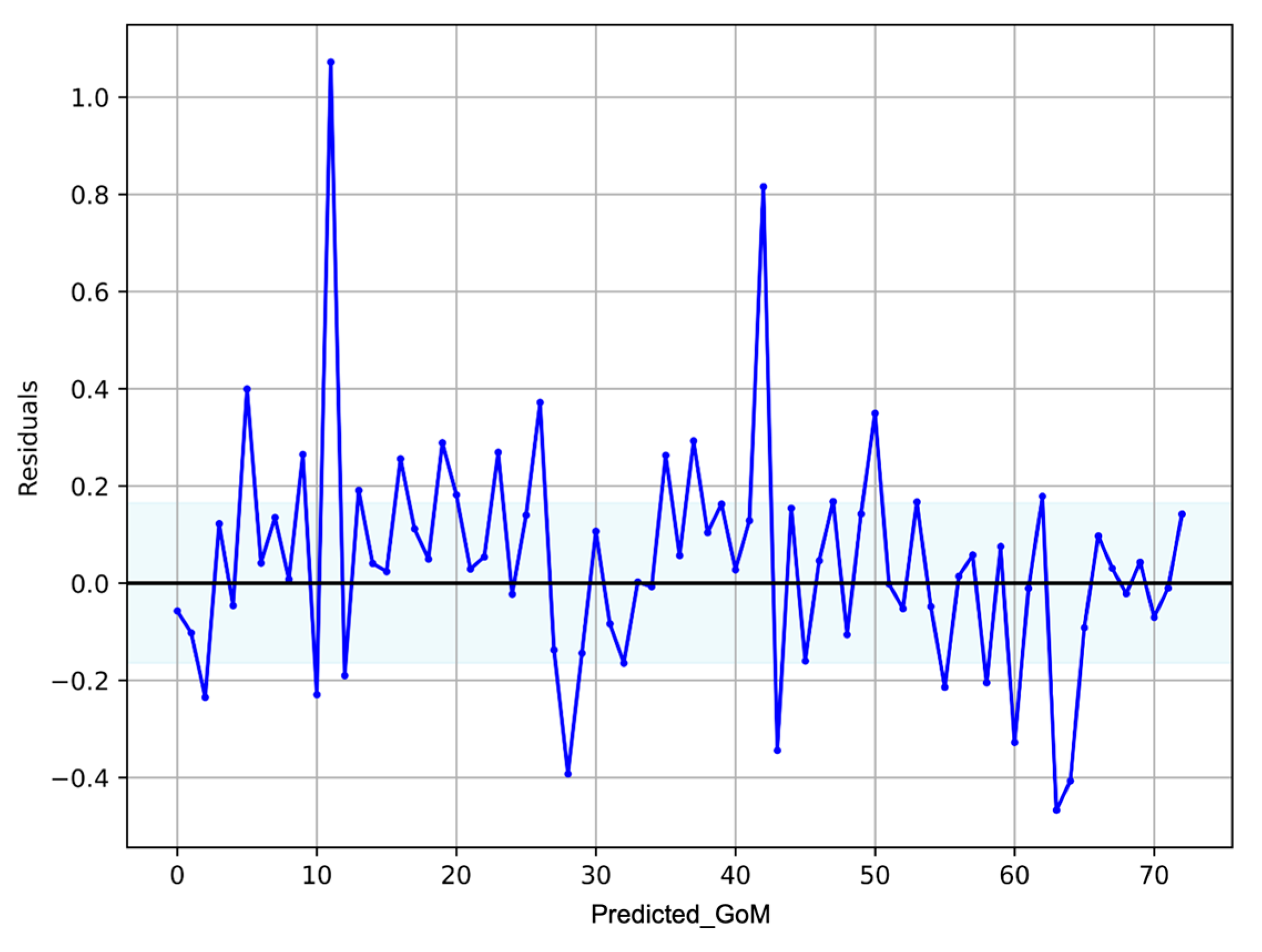
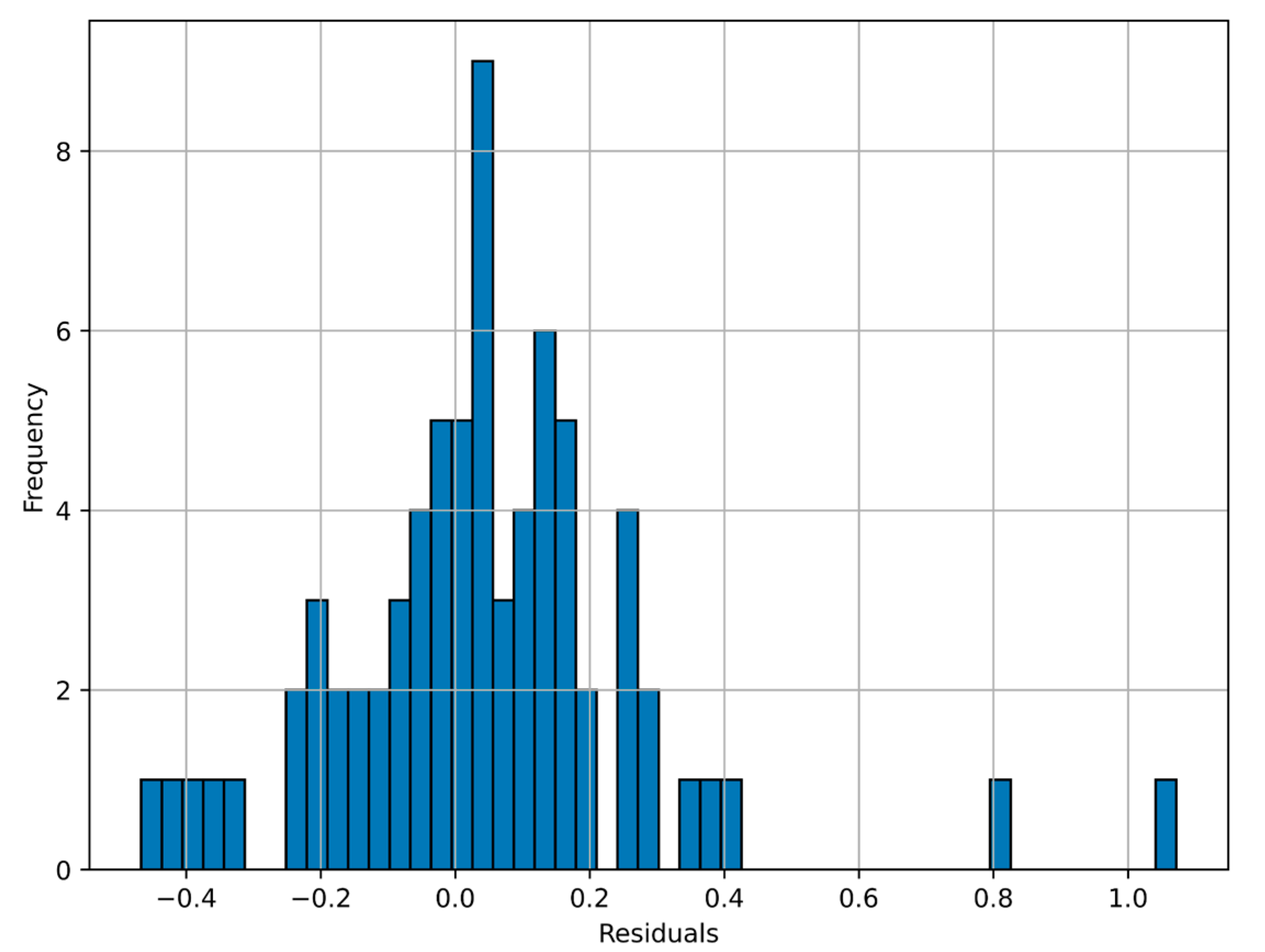
To further assess the model’s error behavior, Figure 12 and Figure 13 illustrate the absolute prediction error and error distribution, respectively. As observed in Figure 10, the model performs reliably for vessels with a G0M of 2 or less, while higher deviations occur for larger G0M values. Figure 11 shows the distribution of absolute errors, with the majority of prediction errors falling below 0.2, suggesting that the model maintains a reasonably tight error margin in most cases.
Based on the validation results described above, it can be concluded that the DNN-based G0M prediction model developed in this study generally demonstrates strong predictive performance. However, the model shows relatively lower accuracy in specific cases, particularly for fishing vessels with actual G0M values exceeding 3.0. Therefore, the model is expected to provide more reliable predictions when applied to vessels with G0M values below 2.0, which aligns with the stability range commonly observed in small fishing vessels. The basis for this assessment is shown in Figure 13, where relatively large errors occur at data indices 11 and 42. In these two cases, the G0M values of the fishing vessels are around 4 m, which are comparatively high. In contrast, the errors are relatively small in the other cases. Furthermore, as illustrated in Figure 9, approximately 80% of the cases show residuals within ±0.2. Considering these points, it can be inferred that the model developed in this study performs more effectively when the G0M values are 2.0 m or less.

5. Conclusions

This study developed a deep neural network (DNN)-based predictive model to estimate the metacentric height (G0M) of small fishing vessels during the early design stage, when only basic hull dimensions are available. Unlike previous research that typically relied on detailed structural drawings or operational data, this model enables preliminary stability assessment using fundamental parameters such as length, breadth, and draft—along with derived ratios—without requiring complete ship plans.
A dataset of 118 Korean fishing vessels under 359 loading conditions was compiled to train and validate the model. The results demonstrate strong predictive performance, with an R2 value of 0.87 and low error levels across MSE, RMSE, and MAE metrics. The model proved especially accurate for vessels with G0M values under 2.0, which are common among small fishing vessels.
This research provides a practical tool for naval architects and designers, enabling early-stage assessment of regulatory compliance and improving design decision-making for small vessels. By integrating AI-based estimation into the design phase, this approach contributes to enhancing vessel safety, efficiency, and adherence to stability standards from the outset. Furthermore, the model’s ability to support efficient, data-driven stability assessment suggests potential applications beyond ship design—particularly in smart port and maritime logistics systems, where automated vessel evaluation can improve planning, safety, and operational integration. Such applicability reinforces the model’s relevance not only to vessel-specific design workflows but also to broader efforts in port automation and intelligent maritime logistics. Such applicability reinforces the model’s relevance not only to vessel-specific design workflows but also to broader efforts in port automation and intelligent maritime logistics.
However, several limitations remain. The present study focused primarily on small vessels, especially fishing vessels designed in Korea, and the dataset was therefore limited in both vessel type and size range. Future work will extend this approach beyond Korean small fishing vessels to include a wider variety of ship sizes and types, enabling broader applicability and validation of the proposed AI-based estimation model.

Author Contributions

Conceptualization, N.I. and Y.J.; validation, Y.J.; writing—original draft preparation, Y.J.; writing—reviewing and editing, N.I. All authors have read and agreed to the published version of the manuscript.

Funding

This research was supported by the Regional Innovation System & Education (RISE) program through the Jeollanamdo RISE center, funded by the Ministry of Education (MOE) and the Jeollanamdo, Republic of Korea (2025-RISE-14-002).

Conflicts of Interest

The authors declare no conflict of interest.

References

  1. International Labour Office; International Maritime Organization; Food and Agriculture Organization of the Uniited Nations. Safety Recommendations for Decked Fishing Vessels of Less than 12 Metres in Length and Undecked Fishing Vessels; International Labour Organization: Genève, Switzerland, 2012; ISBN 978-92-5-107397-1. [Google Scholar]
  2. Enforcement Rules of the Fishing Vessel Safety Operation Act. Available online: https://www.law.go.kr/admRulInfoP.do?admRulSeq=2000000100025 (accessed on 1 September 2025).
  3. Melo, R.F.; Figueiredo, N.M.d.; Tobias, M.S.G.; Afonso, P. A Machine Learning Predictive Model for Ship Fuel Consumption. Appl. Sci. 2024, 14, 7534. [Google Scholar] [CrossRef]
  4. Ren, Y.; Li, X.; Xu, H. Extracting Ship’s Size from SAR Images by Deep Learning. In Artificial Intelligence Oceanography; Li, X., Wang, F., Eds.; Springer: Singapore, 2023. [Google Scholar] [CrossRef]
  5. Latinopoulos, C.; Zavvos, E.; Kaklis, D.; Leemen, V.; Halatsis, A. Marine Voyage Optimization and Weather Routing with Deep Reinforcement Learning. J. Mar. Sci. Eng. 2025, 13, 902. [Google Scholar] [CrossRef]
  6. Balas, E.A.; Balas, C.E. Maritime Risk Assessment: A Cutting-Edge Hybrid Model Integrating Automated Machine Learning and Deep Learning with Hydrodynamic and Monte Carlo Simulations. J. Mar. Sci. Eng. 2025, 13, 939. [Google Scholar] [CrossRef]
  7. Chen, Z.S.; Lam, J.S.L.; Xiao, Z. Prediction of harbour vessel emissions based on machine learning approach. Transp. Res. Part D Transp. Environ. 2024, 131, 104214. [Google Scholar] [CrossRef]
  8. Hasan, S.M.; Islam, M.S.; Awal, Z.I. A Machine Learning Framework for Predicting Efficient Ship Design Parameters. In Proceedings of the 14th International Conference on Marine Technology (MARTEC), Johor Bahru, Malaysia, 24–26 September 2024. [Google Scholar]
  9. He, G.; Xue, J.; Zhao, C.; Cui, T.; Liu, C. Deep learning based short-term motion prediction of floating wind turbine under shutdown condition. Appl. Ocean Res. 2024, 151, 1014147. [Google Scholar] [CrossRef]
  10. Terada, D.; Tamashima, M.; Nakao, I.; Matsuda, A. Estimation of metacentric height using onboard monitoring roll data based on time series analysis. J. Mar. Sci. Technol. 2018, 24, 285–296. [Google Scholar] [CrossRef]
  11. Krata, P.; Wawrzyński, W. Method for ship’s rolling period prediction with regard to non-linearity of GZ curve. J. Theor. Appl. Mech. 2016, 4, 1329–1343. [Google Scholar] [CrossRef]
  12. Wilczynski, V.; Knowles, P.; Diehl, W. Uncertainty Analysis of a Vessel’s Metacentric Height. In Proceedings of the Conference: Probabilistic Safety Assessment and Management—1998, New York, NY, USA, 13–18 September 1998. [Google Scholar]
  13. Ruponen, P.; Manderbacka, T.; Lindroth, D. On the calculation of the righting lever curve for a damaged ship. Ocean Eng. 2018, 149, 313–324. [Google Scholar] [CrossRef]
  14. Perrault, D. Correlations of GZ Curve Parameters. In Proceedings of the 15th International Ship Stability Workshop, Stockholm, Sweden, 13–15 June 2016; pp. 1–7. [Google Scholar]
  15. Kim, D.J.; Yeo, D.J. Estimation of drafts and metacentric heights of small fishing vessels according to loading conditions. Int. J. Nav. Archit. Ocean Eng. 2020, 12, 199–212. [Google Scholar] [CrossRef]
  16. Nam-Kyun, I.M.; Hun, C.H.O.E. A quantitative methodology for evaluating the ship stability using the index for marine ship intact stability assessment model. Int. J. Nav. Archit. Ocean Eng. 2021, 13, 246–259. [Google Scholar]
  17. Woo, D.; Choe, H.; Im, N.-K. Analysis of the Relationship between GM and IMO Intact Stability Parameters to Propose Simple Evaluation Methodology. J. Mar. Sci. Eng. 2021, 9, 735. [Google Scholar] [CrossRef]
  18. Woo, D.; Im, N.-K. A Methodology for Simply Evaluating the Safety of a Passenger Ship Stability Using the Index for the Intact Stability Appraisal Module. Sensors 2022, 22, 1938. [Google Scholar] [CrossRef] [PubMed]
  19. Zhang, M.; Taimuri, G.; Zhang, J.; Hirdaris, S. A deep learning method for the prediction of 6-DoF ship motions in real conditions. Proc. Inst. Mech. Eng. Part M J. Eng. Marit. Environ. 2023, 237, 887–905. [Google Scholar] [CrossRef]
  20. Wang, L.; Liao, S.; Wang, S.; Jia, B.; Yin, J.; Li, R. Real-time prediction of metacentric height of ro-ro passenger ships in Qiongzhou strait based on improved RBF neural network. Ocean Eng. 2024, 312, 119067. [Google Scholar] [CrossRef]
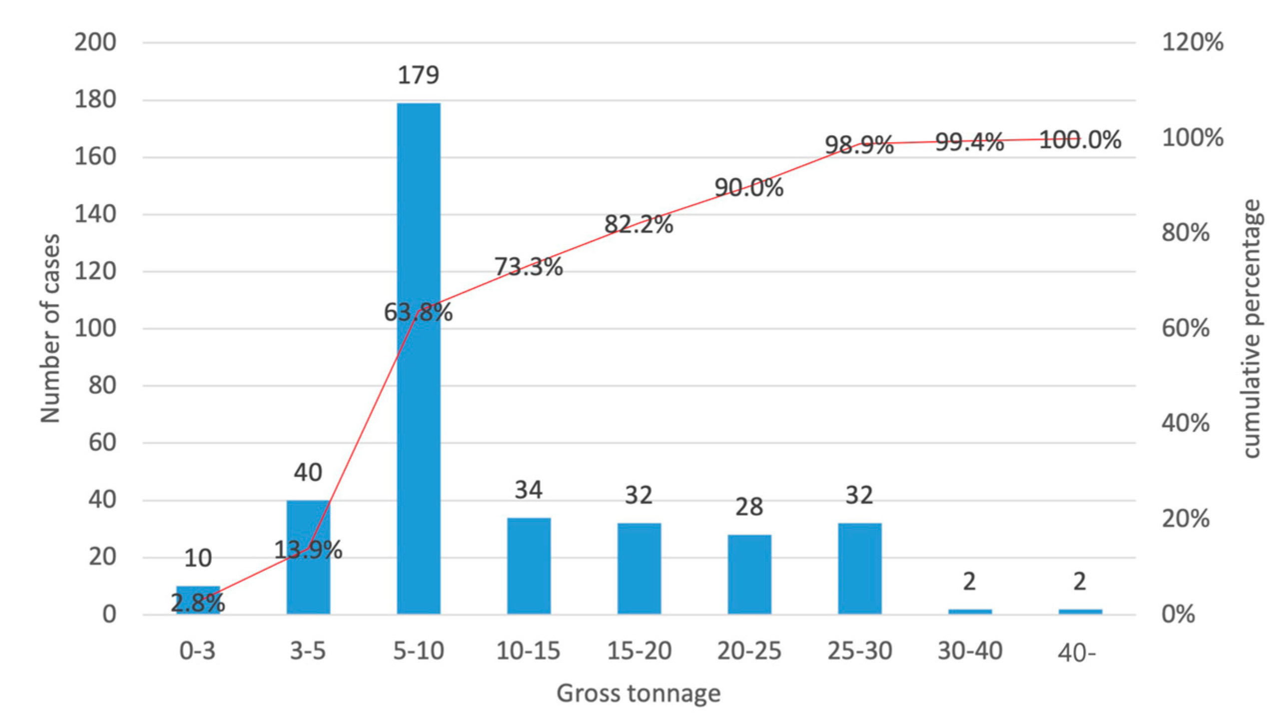
Figure 1. Gross Tonnage of model ships.
Jmse 13 01779 g001
Figure 2. Range of Length and Beam of Ships.
Jmse 13 01779 g002
Figure 3. GZ Curve data for DNN Model.
Jmse 13 01779 g003
Figure 4. Averaged GZ Curve data for DNN Model.
Jmse 13 01779 g004
Figure 5. DNN model structure for G0M Estimation.
Jmse 13 01779 g005
Figure 6. ReLU Activation Function.
Jmse 13 01779 g006
Figure 7. Results of data pre-processing.
Jmse 13 01779 g007
Figure 8. Comparison of Loss Values by Loss Functions (MSE, MAE, Huber).
Jmse 13 01779 g008
Figure 9. Model Loss and Accuracy Graph for Training.
Jmse 13 01779 g009
Figure 10. Comparison between actual and predicted G0M values on the held-out test dataset.
Jmse 13 01779 g010
Figure 11. Comparison of Actual and Predicted Values of G0M Values.
Jmse 13 01779 g011
Figure 12. Residual Errors of G0M Model.
Jmse 13 01779 g012
Figure 13. Residual Histogram for The G0M Prediction Model.
Jmse 13 01779 g013
Table 1. Stability Criteria of the Torremolinos International Convention.
CriteriaMinimum Requirement
G0M (metacentric height)0.35 m
(0.15 m for vessels ≥ 70 m in length or with significant upper structures)
GZ (Righting Lever) at 30° heel angle0.2 m
Angle Max GZ25°
GZ Curve AreaBetween 0° and 30°0.055 m-rad
Between 0° and 40° or ϕ f   10.090 m-rad
Between 30° and 40° or ϕ f 0.030 m-rad
1  ϕ f : The angle at which water ingress begins (the angle at which openings in the hull, superstructure, or deckhouse—that cannot be rapidly and effectively closed to ensure watertight integrity—start to become submerged).
Table 2. Domestic Stability Regulations for Fishing Boat.
Vessel TypeCriteria
Vessels 24 m or more but less than 40 m in length 0.04 B + α B D β   ° m ≤ G0M
Vessels 40 m or more in length0.35 m ≤ G0M
(0.15 m for vessels with traditional superstructures or those 70 m or more in length)
G Z 30 0.2 m
Maximum GZ Angle25°
GZ Area0–30°0.055 m-rad
0–40°0.090 m-rad
Weather
Criterion
30–40°0.030 m-rad
Area Ratio
(b/a)
1
Heel angle under steady windLimit of heel angle or not exceeding 16°
Table 3. Details of ship specification Features in DNN model.
NoFeatures (Unit)
1LOA (m)
2LBP (m)
3Draft (m)
4Breadth (m)
5Depth (m)
6Light Weight Tonnage (ton)
7Dead Weight Tonnage (ton)
8Displacement (ton)
9Cb (-)
10LBP × B (m × m)
11LBP × D (m × m)
12B × d (m × m)
13L/B (-)
14B/d (-)
15L/d (-)
16D/B (-)
Table 4. Training Hyperparameter.
HyperparameterValue
Train:Test8:02
Hidden Layer128:256:128
Dropout0.3
Loss FunctionHuber
OptimizerAdam
Learning rate0.001
Batch size32
epoch1000
Table 5. Evaluation Metrics for Estimation G0M Model.
MetricDescriptionValue
R 2 scoreCoefficient of determination0.8701
MSEMean Squared Error0.0577
RMSERoot Mean Squared Error0.2402
MAEMean Absolute Error0.1647
Disclaimer/Publisher’s Note: The statements, opinions and data contained in all publications are solely those of the individual author(s) and contributor(s) and not of MDPI and/or the editor(s). MDPI and/or the editor(s) disclaim responsibility for any injury to people or property resulting from any ideas, methods, instructions or products referred to in the content.