Article

Estuary-Tidal Residual Water Level Forecasting Method Based on Variational Mode Decomposition and Back Propagation Neural Network

by
Min Zhai
1,
Qihang Cao
1,
Pengfei Huo
1,
Xintong Du
1 and
Mingzhen Xin
1,2,*
1
College of Geodesy and Geomatics, Shandong University of Science and Technology, Qingdao 266590, China
2
Key Laboratory of Ocean Geomatics, Ministry of Natural Resources of China, Qingdao 266590, China
*
Author to whom correspondence should be addressed.
J. Mar. Sci. Eng. 2025, 13(9), 1755; https://doi.org/10.3390/jmse13091755
Submission received: 15 July 2025 / Revised: 6 September 2025 / Accepted: 9 September 2025 / Published: 11 September 2025
(This article belongs to the Section Coastal Engineering)

Abstract

The water level changes in the estuarine area are influenced by various factors with different mechanisms and periodicities, including runoff, astronomical tides and storm surges, resulting in relatively low forecasting accuracy of the residual water level. To improve the forecast accuracy of residual water levels, an estuary-tidal residual water level forecasting method based on VMD-BPNN (variational mode decomposition and back propagation neural network) is proposed. By conducting tidal harmonic analysis on the long-term water level data of estuarine areas, astronomic water levels and residual water levels can be obtained. The residual water level is subjected to VMD, obtaining multiple intrinsic mode functions of the residual water level in the time series. Then, the BPNN is used to train each intrinsic mode function, and an accurate forecast of residual water levels in the estuary area is achieved through the forecast and superposition of each intrinsic mode function. Water level data from four typical tidal stations in estuarine areas of the United States and France were used for experimental analysis. The method was verified by using Root Mean Square Error (RMSE), Mean Absolute Error (MAE) and Nash-Sutcliffe Efficiency (NSE) as evaluation indicators, and the results showed that it had a good comprehensive performance, and high stability and accuracy in the forecasting of the residual water level. This study thereby provides a valuable foundation and insightful reference for future research into the complex mechanisms driving water level changes and the development of high-precision tidal forecasting systems in estuarine environments.

1. Introduction

Tides are a periodic deformation and oscillation phenomenon of the sea level [1], the Earth’s crust, and the atmosphere caused by the combined effects of the gravitational forces of celestial bodies (primarily the Moon and the Sun) and the centrifugal force caused by the Earth’s orbital motion around its center of mass. They play a crucial role in the Earth’s ecosystem and economic activities, as well as in disaster warning. Tidal fluctuations are composed of multiple components, among which the astronomical tides (including solar tides, lunar tides, etc.) are the most significant periodic changes [2], while non-periodic influences, such as storm surges, pressure changes, variations in watershed water volume, and other factors, may cause sudden, unexpected changes in water levels or fluctuations [3]. The residual water level of tides refers to the residual water level after removing the effects of regular astronomical tides or influenced by tidal fluctuations. Its formation is related to topography, weather, and climate factors, and it is also known as the disturbed water level, which can reflect additional water level changes beyond the tides [4]. Tidal-induced basal water level changes can significantly amplify extreme water level events caused by storm surges, rainfall, and sea-level rise, and are key contexts and amplifying factors for assessing coastal flood risk. Magoulick et al. [5] developed a novel ENSO-incorporated statistical model (ENSO-JPMM) that significantly improves extreme water level forecast accuracy in Annapolis, revealing climate-related flood risks that are potentially underestimated by conventional methods.
The water level changes in estuarine areas are influenced not only by astronomical tides but also by a combination of factors such as inland runoff, meteorological conditions (like air pressure, wind strength, wind direction, etc.), and topography. The interactions among these irregular change factors are complex and variable, making it difficult to accurately grasp the patterns of tidal residual water levels [6], which complicates the forecasting of residual water levels and results in relatively low forecasting accuracy for tidal residual water levels in estuarine areas at this stage.
With regards to tidal analysis, Loh et al. [7] used empirical mode decomposition (EMD) as a decomposition method and employed artificial neural network forecast models to explore the impact of EMD on water level forecasting. Wu et al. [8] studied the calculation of storm surges based on the ensemble empirical mode decomposition (EEMD) algorithm, discussing the possibility of separating storm surges in a short-term time series evaluation of the sea level. However, a large number of studies have shown that EMD can encounter issues such as mode mixing, endpoint effects, and tidal period overlap, which pose limitations for tidal extraction, noise suppression, and long-term trend analysis [9]. Although EEMD partially resolves the modal aliasing problem of EMD, it still has issues with computational efficiency, residual noise, and physical interpretability [10]. Variational mode decomposition (VMD) is a completely non-recursive signal decomposition method that achieves signal decomposition through mathematical optimization of constrained modal bandwidth and center frequency. On the one hand, VMD enforces the independent distribution of different frequency components by presetting the number of modes and bandwidth constraints, effectively addressing the issue of modal aliasing [11]. On the other hand, the VMD process is based on the intrinsic frequency characteristics of the signal, making it highly robust to noise [12]. Therefore, compared to EMD and EEMD, VMD can suppress random noise while preserving weak tidal components such as shallow water tidal and long-period tidal components [13], which is crucial for tidal analysis in areas with low signal-to-noise ratios such as estuaries or nearshore shallow waters.
In terms of tidal water level forecasting, the interactions between ocean currents, tides, and the seabed topography are very complex, which means that the forecasting models for tidal residual levels are often affected by many uncertainties [14]. Although some existing numerical simulation methods (such as finite element methods, three-dimensional hydrodynamic models, etc.) can partially forecast tidal residual levels [15], they typically require a large amount of measured data and high-performance computing resources. Tidal harmonic analysis is a classic water level forecasting method based on astronomical tidal components and tidal frequencies [16]. However, it cannot accurately reflect changes in water levels caused by non-astronomical factors and relies on long-term stable tidal patterns, showing lower sensitivity to short-cycle or localized disturbances (such as internal waves and river runoff). In recent years, deep learning technologies have demonstrated stronger adaptability in tidal and water level forecasting [17]. Ueda et al. [18] use a deep learning model based on radar rainfall data to forecast river water levels, building a forecast model that combines two-dimensional convolutional neural networks and long short-term memory networks to leverage the spatial and temporal features of radar rainfall data. Kim et al. [19] established the Long Short-Term Memory (LSTM) model to forecast the water levels at various stations in the southern part of the Nam Ou River basin based on rainfall and water level data observed in previous time periods. Li et al. [20] investigated the application and performance of four different deep learning models in forecasting water levels. Sun et al. [21] proposed a new method called TidalMet-HR, which achieved accurate forecasting of residual water levels by inputting wind speed, wind direction, air pressure, and historical residual water level data into a bidirectional long short-term memory network. Stojković et al. [22,23] assessed the impact of climate change on water resources, identified significant trend harmonics using discrete spectral analysis, and proposed a new trend evaluation method that takes into account the long-term periodicity of annual flow.
The difficulty of forecasting the residual water level in an estuary lies in the nonlinear coupling of runoff, tide and meteorological factors, the large spatiotemporal variation in meteorological forcing (wind and pressure), the complex separation and modeling of non-astronomical tidal components, and the uncertainty of model parameterization. In order to further improve the forecast accuracy of the residual water level in estuary areas, an analysis and forecasting method based on VMD-BPNN is proposed. The variational mode decomposition of the residual water level is carried out to obtain the intrinsic mode function of the residual water level in the time series. Then, the fast Fourier transform (FFT) is used to analyze the spectral characteristics of each intrinsic modal function, and then the back propagation neural network is used to train each intrinsic modal function to forecast the residual water level in different time periods. The organization of the paper is as follows: Section 2 describes the VMD-BPNN analysis and forecast methods for estuarine tidal residual water levels, as well as the specific estuarine areas studied and the tidal and water level data sources used. In Section 3, the experimental analysis of VMD and the forecast of residual water level was carried out. Section 4 summarizes the role of the VMD-BPNN combined model in forecasting the tidal residual water level in estuarine areas.

2. Data and Method

2.1. Research Areas and Data

The experiment selected tidal water level data from two tide gauge stations in the United States, Sabine Pass and Pilottown, from 1 January 2022 to 31 December 2023, as well as tidal water level data from two tide gauge stations in France, Saint-Nazaire and Saint-Malo, from 1 January 2017 to 31 December 2018. Figure 1 shows the locations of the two tide gauge stations in the United States and the two in France.
(1)
The Sabine Pass tidal gauge station is located in the southeastern part of Texas, at the confluence of Sabine Lake and the Gulf of Mexico, close to the Louisiana border. It is a typical estuarine wetland environment, characterized by low-lying terrain influenced by the Mississippi River delta plain.
(2)
The Pilottown tidal gauge station is located at the southernmost tip of the Mississippi River Delta in Louisiana, close to the river’s mouth. This station is situated in a highly dynamic sedimentary environment, surrounded by ever-changing river channels, swamps, and lagoons, with very low terrain significantly affected by river sedimentation and erosion.
(3)
The Saint-Nazaire tidal gauge station is located on the southern bank of the Loire estuary on the west coast of France, adjacent to the Bay of Biscay. The station is situated in the open waters of the eastern Atlantic, affected by both Atlantic swells and estuarine topography.
(4)
The Saint-Malo tidal gauge station is located on the northern coast of the Brittany region in France, at the junction of the English Channel and Saint-Malo Bay. The narrow topography of the bay and the resonance effect enhance the tidal amplitude.
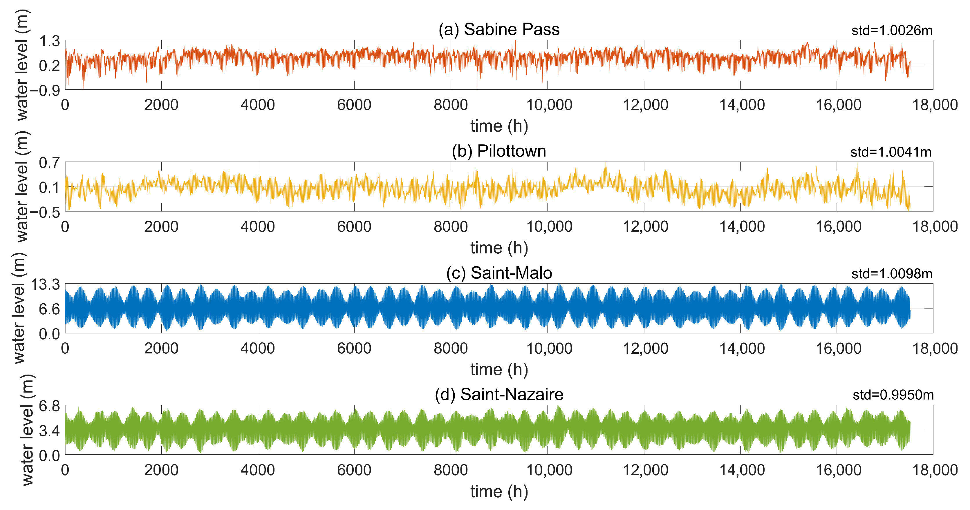
Figure 2 shows the original water level data from four tidal gauge stations.

2.2. Tide Harmonic Analysis

The basic principle of tidal harmonic analysis is to use mathematical models to break down complex tidal phenomena into a series of periodic constituent tides [24]. These constituents are caused by the gravitational effects of celestial bodies, with each constituent having specific periods, amplitudes, and phases. Through tidal harmonic analysis, the main factors influencing tides can be identified and the corresponding harmonic constants can be calculated.
The observed water level h ( t ) can be represented as a linear superposition of multiple tidal components:
h t = M S L + i = 1 m H i cos V i t g i + R t + Δ t
where M S L is the mean sea level; m is the number of tidal constituents; H and g are the harmonic constants of the tidal constituents; V ( t ) is the astronomical phase angle of the tidal constituents at time t ; R ( t ) is the residual water level; Δ t is the measurement error expected to be zero.
The goal of harmonic analysis is to calculate the harmonic constants H and g of each tidal component from the above equation with M S L . Considering the water level changes as a signal, the harmonic constants H and g of the tidal components can be viewed as the amplitude and phase delay of fluctuations with known periods, while the average sea level at the zero point of the water level M S L can be seen as the systematic deviation of the fluctuations. By using the method of least squares fitting to solve for H and g , the residual water level can be obtained.
R t = h t M S L i = 1 m H i cos V i t g i
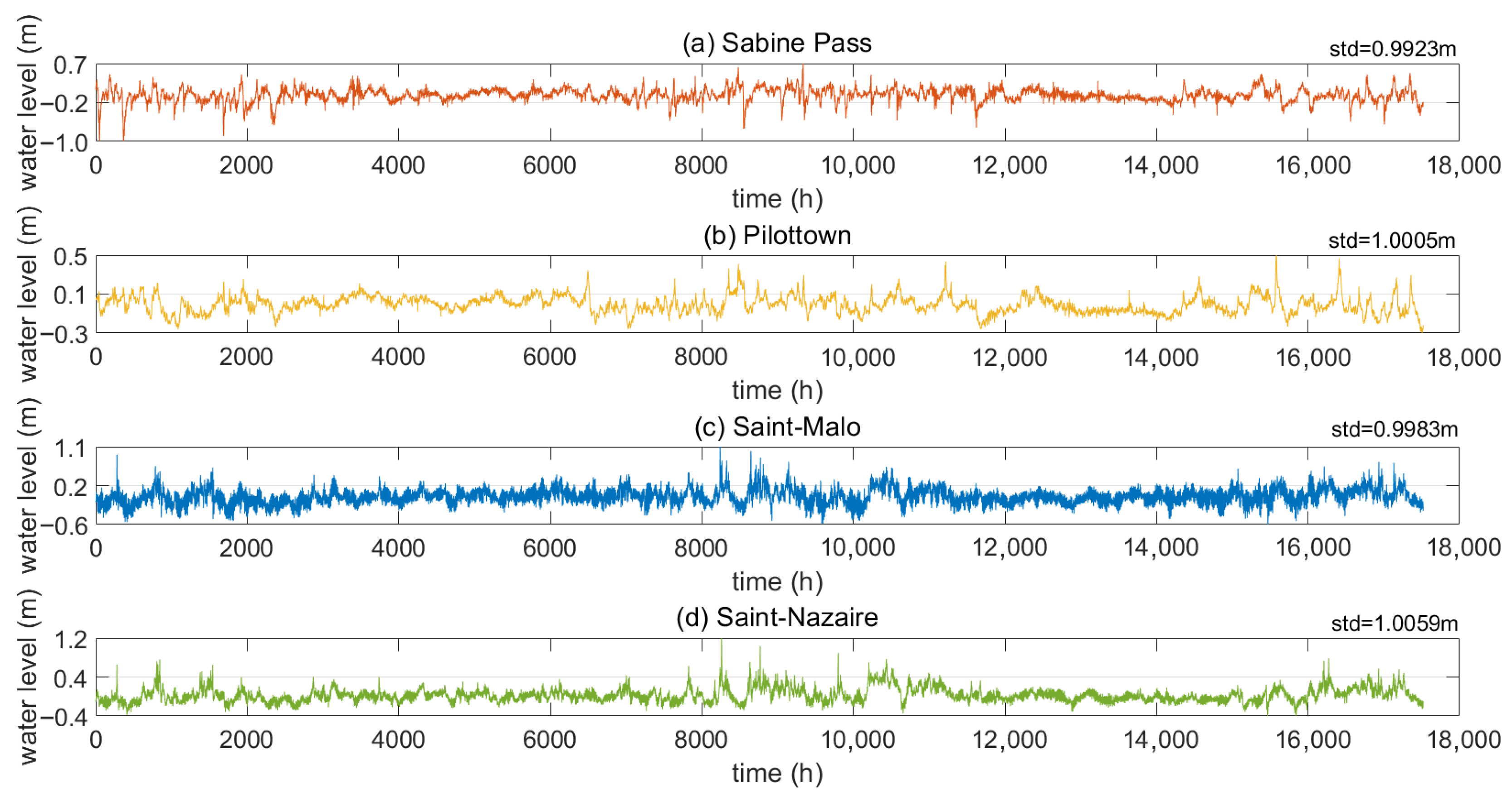
A classical harmonic analysis of the water level data of each station for 2 years was carried out, and 68 harmonic components such as half-diurnal tide, diurnal tide, shallow water tide, and long-period tide were extracted, which effectively eliminated the tidal in-fluence in the original water level data within a 95% confidence interval. Among them, the 13 major ones are as follows: Principal Lunar Semidiurnal Constituent (M2), Principal Solar Semidiurnal Constituent (S2), Lunar Elliptical Semidiurnal Constituent (N2), Luni-Solar Semidiurnal Constituent (K2), Luni-Solar Diurnal Constituent (K1), Principal Lunar Diurnal Constituent (O1), Principal Solar Diurnal Constituent (P1), Lunar Elliptical Diurnal Constituent (Q1), Principal Lunar Long-Period Constituent (Mf), Lunar Monthly Long-Period Constituent (Mm), Solar Semi-annual Long-Period Constituent (Ssa), Solar Annual Long-Period Constituent (Sa), and Principal Lunar Quarter-Diurnal Constituent (M4). In classical tidal harmonic analysis, these 13 major components form the core of tidal motion, while the rest are mostly minor or shallow water components that contribute little to total tidal variation. Subsequently, by calculating the difference between the observed water levels and the astronomical tidal forecasts, the residual water levels were obtained. Figure 3 displays the residual water level data from the four tidal gauge stations.

2.3. Variational Modal Decomposition

The principle of VMD is mainly based on the variational framework in signal processing, used to decompose complex signals into multiple Intrinsic Mode Functions (IMFs) with fixed center frequencies and finite bandwidths [25]. This method assumes that any signal is composed of a series of sub-signals with specific center frequencies and finite bandwidths.
The constructed VMD constrained variational model is as follows:
min u k , ω k k = 1 K t δ t + j π t u k t e j ω k t 2 2
The constraints are as follows:
k = 1 K u k t = f t
where u k t is the k-th modal component; ω k is the center frequency of the k-th mode; K is the number of modes; t is the partial derivative computation symbol; δ t is the Dirac delta function; t + j π t u k t represents the Hilbert transform of u k t , obtaining the analytic signal; e j ω k t shifts the modal spectrum to baseband to facilitate bandwidth calculation.
Introduce the constraints into the objective function to construct the augmented Lagrangian function.
L u k , ω k , λ = α k = 1 K t δ t + j π t u k t e j ω k t 2 2 + f t k = 1 K u k t 2 2 + λ t , f t k = 1 K u k t
where λ t is the Lagrange multiplier, and α is the quadratic penalty parameter.
For each modality u k , update in the frequency domain using Wiener filtering:
u ^ k n + 1 ω = f ^ ω i k u ^ i ω + λ ^ ω 2 1 + 2 α ω ω k 2
where f ^ ω , u ^ i ω , and λ ^ ω are the Fourier transforms.
Take the mean of the instantaneous frequency of the modal as the new center frequency:
ω k n + 1 = f 0 ω | u ^ k ω | 2 d ω f 0 | u ^ k ω | 2 d ω
Finally, obtain K modal components u k t k = 1 K and their center frequencies ω k k = 1 K , ensuring that each mode is compactly distributed around ω k in the frequency domain, and that the sum of all modes precisely reconstructs the original signal.

2.4. Back Propagation Neural Network

The back propagation neural network is one of the most commonly used artificial neural networks [26], widely applied in areas such as pattern recognition, data forecasting, and image processing. It is a type of feedforward neural network consisting of an input layer, hidden layers, and an output layer. The input layer is designed to receive input data, with each node representing an input feature. One or more hidden layers are employed to learn the complex features of the data. The number of nodes in the hidden layers and the number of layers themselves are hyper-parameters determined during the design phase, which affect the learning capability of the network. Depending on the specific task, the number of nodes in the output layer dictates the dimensionality of the output. The core idea of the back propagation neural network is to optimize the weights and biases in the network through the back propagation algorithm, thereby making the network outputs closer to the expected values.
L-layer neuronal weighted inputs:
z ( l ) = w ( l ) a ( l 1 ) + b ( l )
Activation output:
a ( l ) = σ ( z ( l ) )
where w ( l ) is the weight matrix, a ( l 1 ) is the front-layer output, and σ is the activation function.
Output layer error term:
δ ( L ) = a C σ ( z ( L ) )
Hidden layer error term:
δ ( l ) = ( W ( l + 1 ) ) T δ ( l + 1 ) δ ( z ( l ) )
where C is the loss function, a C is the gradient of the loss to the output, and is the element-by-element multiplication, and the error is transmitted layer by layer through the chain rule.
Weight update:
Δ W ( l ) = η δ ( l ) ( a ( l 1 ) ) T
where η is the learning rate, and the weight is adjusted by gradient descent to minimize the loss function.
Forward propagation calculates the output, back propagation is based on the loss gradient, the weight gradient is calculated layer by layer using the chain rule, and finally the parameters are updated by gradient descent.

2.5. Evaluation Indicators

RMSE, MAE and NSE indicators are used for accuracy assessment, as shown in the following formulas.
R M S E = 1 N i = 1 N y i y ^ i 2
M A E = 1 N i = 1 N | y i y ^ i |
N S E = 1 i = 1 N y i y ^ i 2 i = 1 N y i y ¯ 2
where y is the observed value; y ^ is the forecasted value; y ¯ is the average of observations; N is the number of samples.
RMSE is the standard deviation of forecast error, which has a stronger penalty effect on larger forecast errors and is the most commonly used index to measure forecast accuracy. MAE is the average of the absolute value of the forecast errors for all individuals, which can intuitively reflect the overall level of forecast errors. NSE measures the forecasting power of a model by comparing model forecasts with simply using the mean to measure the pros and cons of forecasts, with values closer to 1 indicating that the model is more effective.

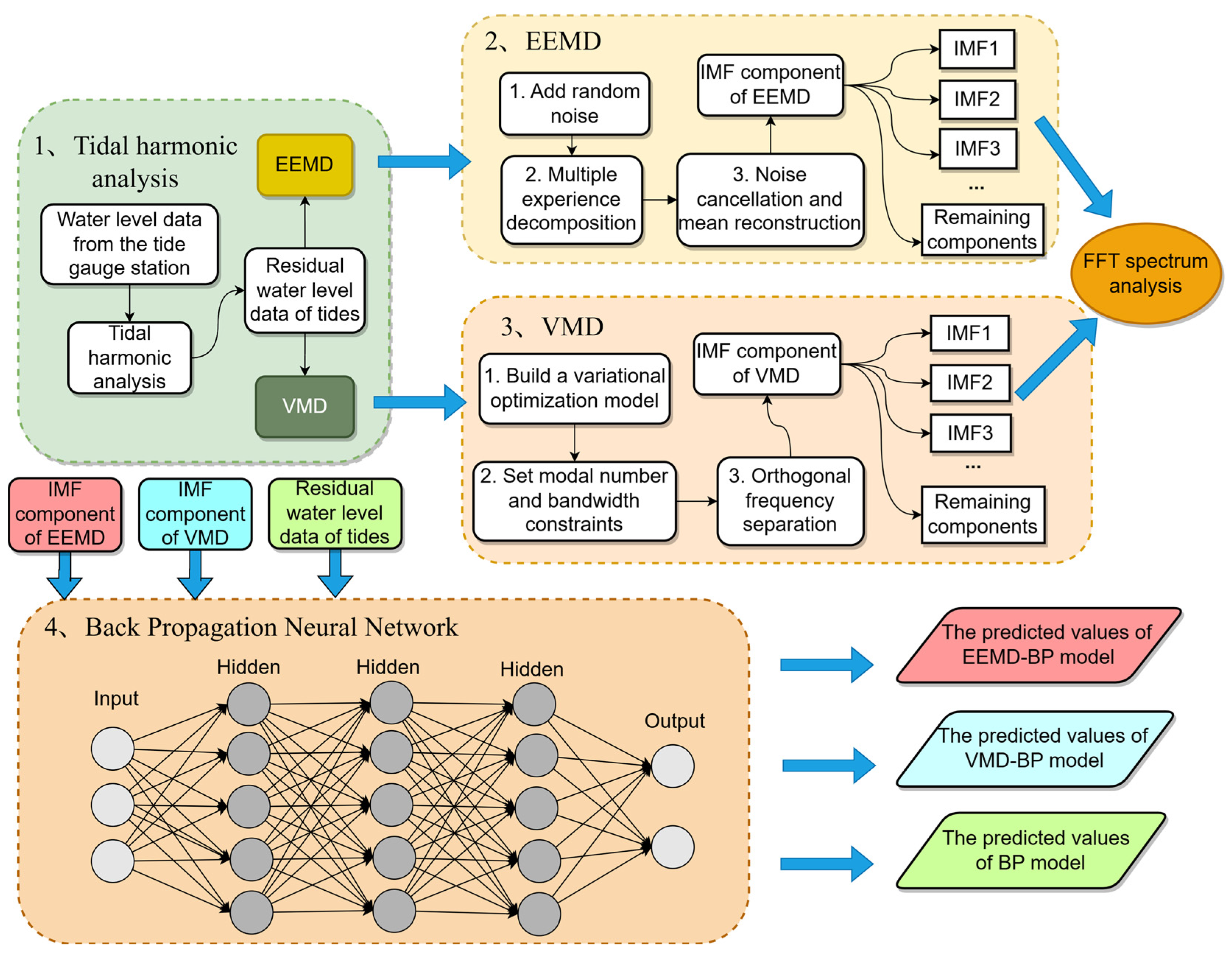
2.6. Processing Flow of VMD-BPNN

An estuary-tidal residual water level forecasting method based on VMD and BPNN is proposed, and the process of the method is as follows:
(1)
Conduct tidal harmonic analysis on the water level data of the tide gauge station.
(2)
Use VMD and EEMD methods to decompose the sequence, resulting in several IMFs and a residual component.
(3)
Analyze the spectral characteristics of each component.
(4)
Finally, train these components using a back propagation neural network and forecast backward. The forecasted results of each component are added to obtain the forecasted value of the residual water level.
The specific process is shown in Figure 4.

3. Results and Discussion

3.1. VMD Experimental Analysis

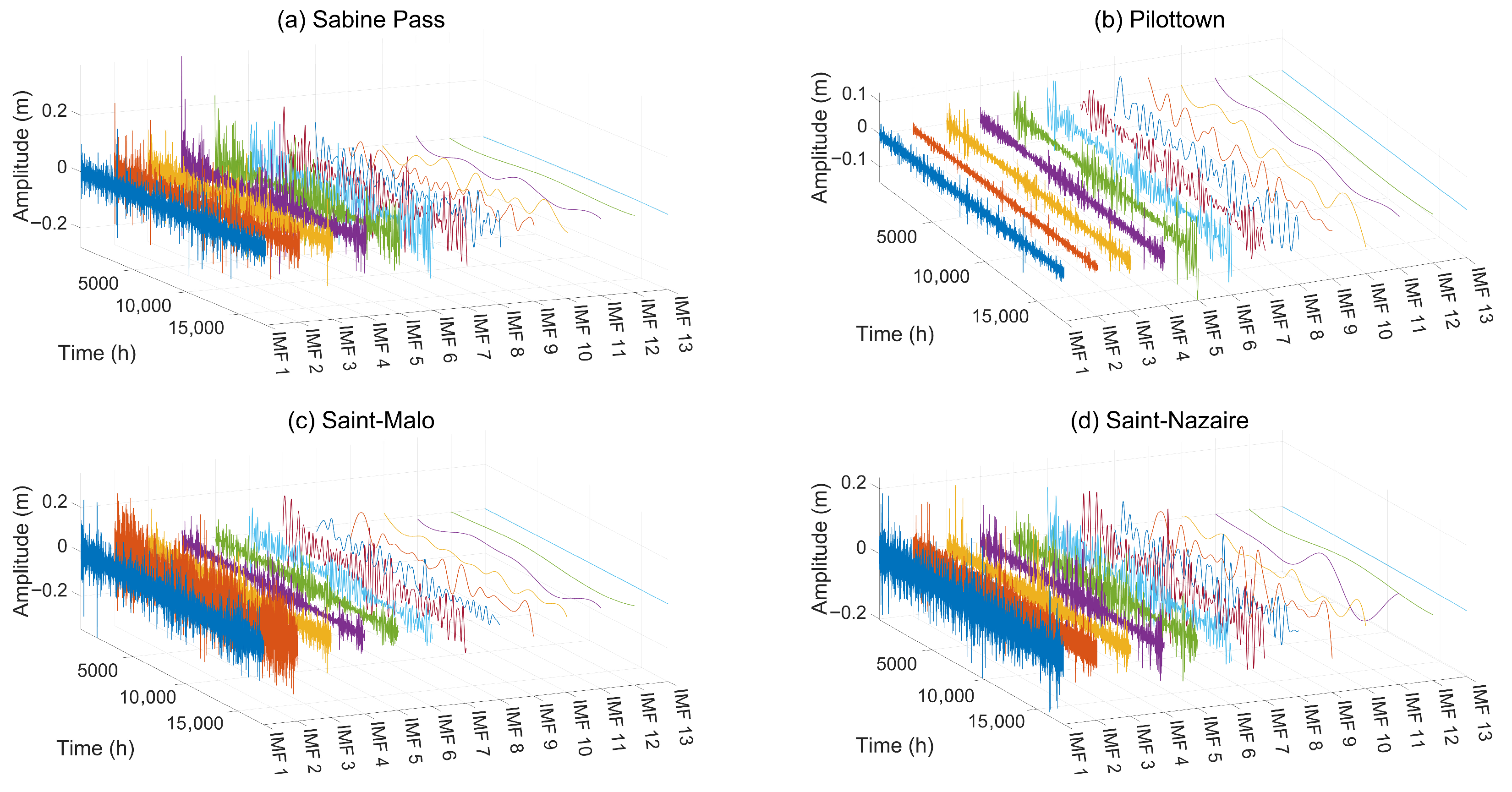
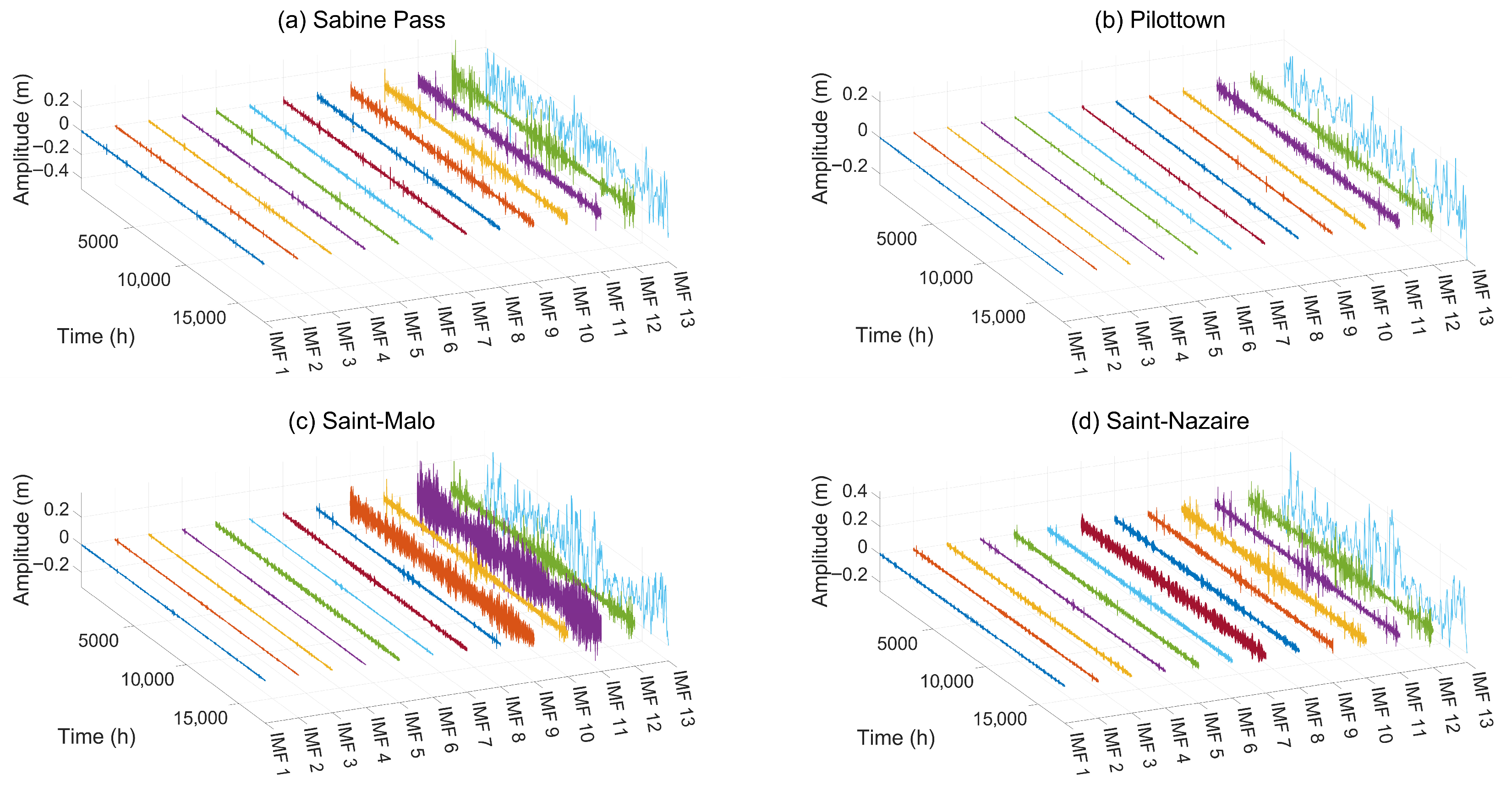
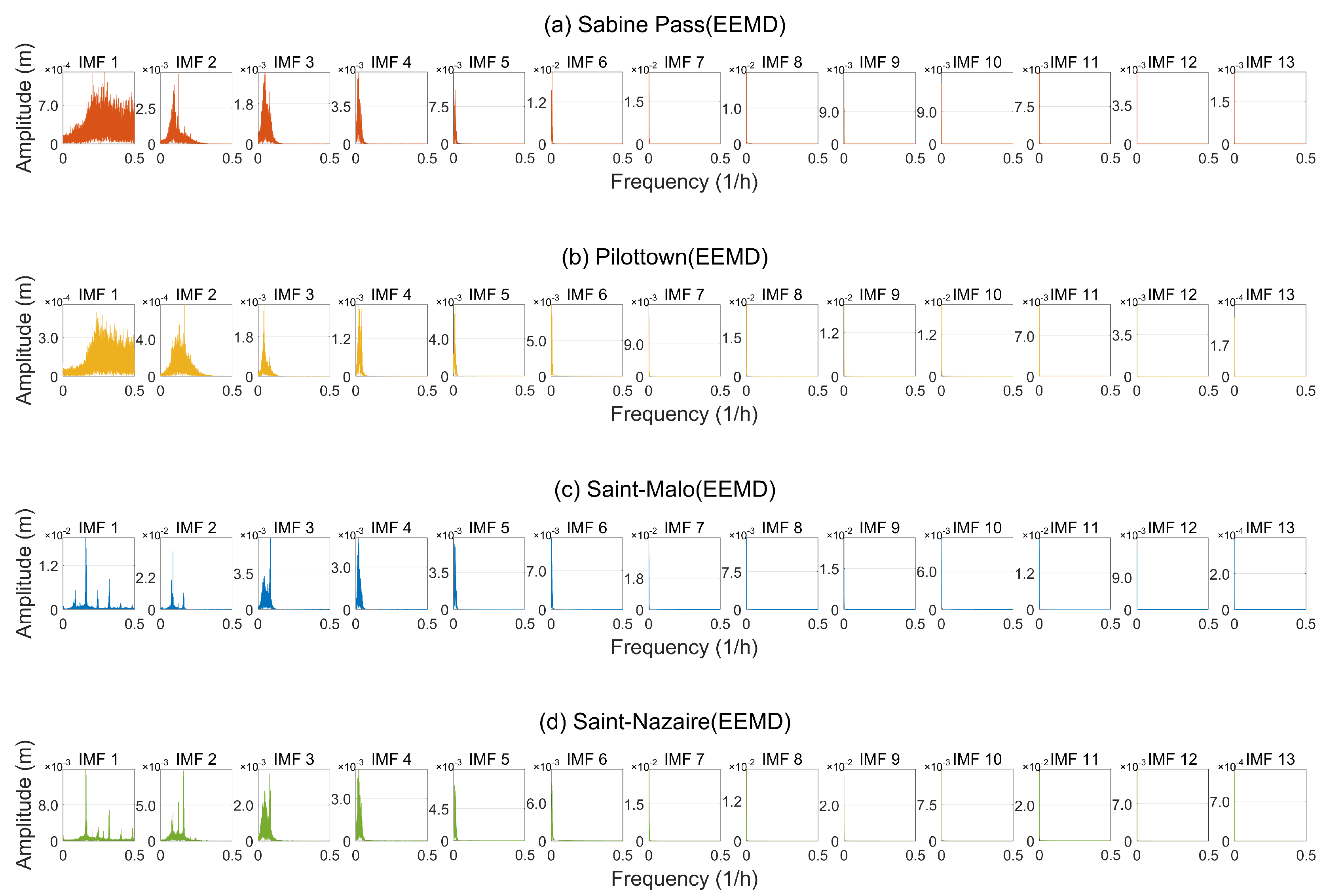
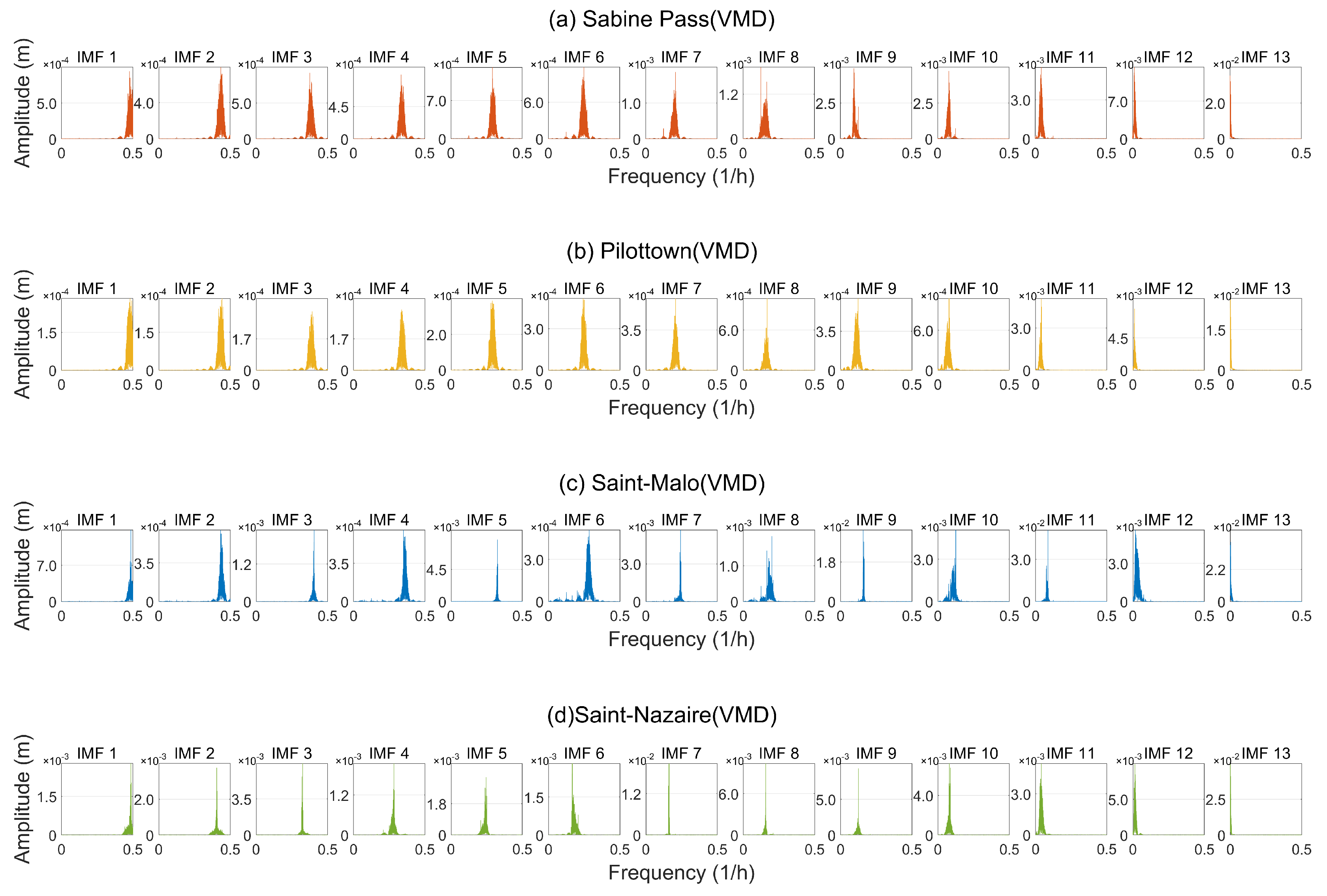
By decomposing the residual water level signal using EEMD and VMD, we obtain thirteen IMFs and one residual component. Each IMF corresponds to a frequency component of the residual water level, usually exhibiting different frequency characteristics. At this point, FFT analysis can be performed on each IMF to understand its frequency characteristics. By observing the frequency spectrum of each mode, we can derive the distribution of its frequency components. FFT is an efficient algorithm for computing Fourier transforms, enabling the conversion of signals from the time domain to the frequency domain. FFT provides a representation of the signal in frequency space, revealing the spectral characteristics of the signal. Figure 5 and Figure 6 are the EEMD graph and the VMD graph, respectively; Figure 7 and Figure 8 show the frequency graphs after FFT of EEMD and VMD, respectively.
The analysis of the experimental results is as follows:
(1)
From Figure 5, it can be seen that the residual water level signal obtained multiple IMFs after EEMD. Each mode exhibits a certain adaptability in the time–frequency domain, but there is a modal aliasing phenomenon in the high-frequency part, manifested as overlapping frequency bands of adjacent modes, and some IMFs contain residual noise. This indicates that while EEMD suppresses the instability of single EMD through noise perturbation, its decomposition results are still affected by the number of ensemble averages and the amplitude of noise, which may lead to the loss of detailed information.
(2)
As shown in Figure 6, VMD achieves accurate separation of signals through preset modal numbers and constrained variational problems. The amplitude and frequency distribution of low-frequency and high-frequency modes show significant differences, indicating that VMD has stronger robustness in processing non-stationary signals, effectively preserving local features of the signal.
(3)
Comparing Figure 5 and Figure 6, it can be observed that, compared to EEMD, VMD adaptively optimizes the central frequency and bandwidth of modes through a variational framework, avoiding the modal uncertainty introduced by noise-assisted methods. Furthermore, it can still accurately separate tidal multi-scale periodic components under strong noise interference, with significantly better physical interpretability and resistance to modal aliasing than EEMD.
(4)
From Figure 7, it can be seen that each IMF of EEMD exhibits a multi-peak distribution characteristic in the frequency domain, reflecting the complex periodic fluctuations in the signal (such as tidal and runoff superposition). Some IMFs show overlapping spectra, manifested as overlapping peaks in adjacent frequencies or noise interference. The main frequency components are identifiable, but background noise is quite pronounced.
(5)
As indicated in Figure 8, the frequency graph of VMD after FFT shows a higher degree of frequency separation, with each mode having a clear central frequency in the frequency domain, and the bandwidth being controllable, effectively avoiding the issue of modal aliasing. This demonstrates that VMD, through its framework of constrained bandwidth optimization, can more effectively extract the inherent modal components of the signal, suppressing modal aliasing and unrelated noise interference.
(6)
Comparing Figure 7 and Figure 8, it can be seen that EEMD, relying on multiple averaging of random noise, leads to the loss of high-frequency details and introduces additional noise, while VMD shows clearer modal separation characteristics, with defined frequency boundaries for each component and significantly reduced modal aliasing. At the same time, VMD effectively suppresses noise interference through preset bandwidth constraints, resulting in stronger frequency energy focusing and enabling a more precise extraction of the multi-scale periodic characteristics of tidal residual water levels.

3.2. Experimental Analysis of the Forecast of Residual Water Level

In this study, the time series data, with a total length of 17,520 h, was divided into three parts: the first 68% of the data was used as the training set for model training; the middle 12% of the data was used as the validation set for hyper-parameter tuning and early stop; and finally, the last 20% of the data was used as a test set to evaluate the general performance of the model, which was not used at all during the training process. All performance metrics reported in this article were calculated based on this test sequence. The activation function for the hidden layer is ‘Tansig’, and for the output layer, it is ‘Purelin’. The minimum global error was set to 0.0001, the learning rate was 0.01, the number of hidden layer nodes was 30, and the maximum number of training iterations was 500. BPNN, EEMD-BPNN, and VMD-BPNN were used for forecasting residual water levels.
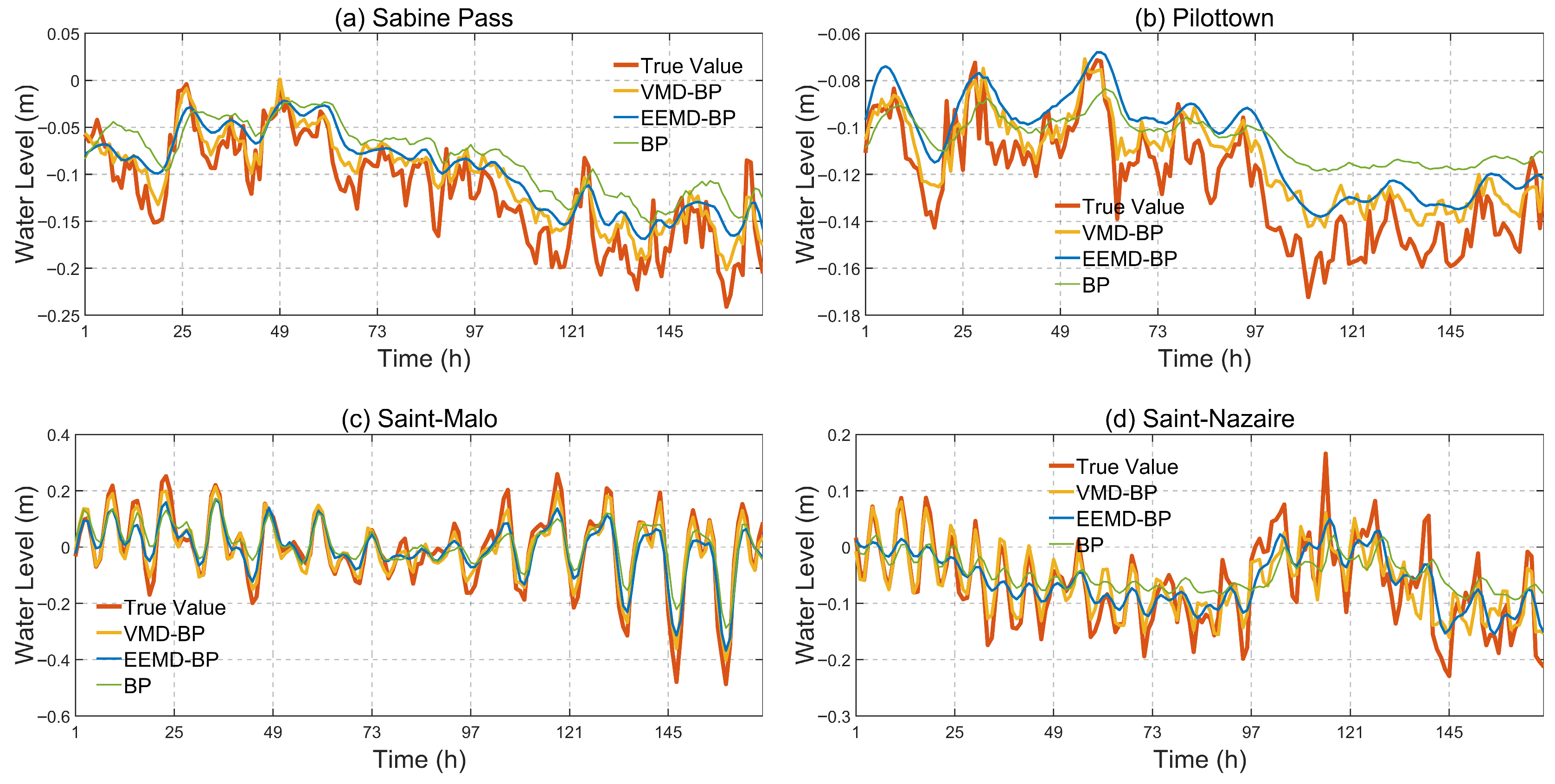
The forecasted values of three residual water levels obtained were compared with the residual water level values obtained through tidal harmonic analysis, resulting in comparison graphs for the three forecasted values and true values over a month for four stations, as well as tables showing the forecast accuracy of residual water levels at each station. Figure 9, Figure 10 and Figure 11 show the comparison of forecasted and true values for four tidal stations over the course of a month, a week, and a day, respectively. Table 1 shows the forecast accuracy of the residual water levels at each station.
The analysis of the experimental results shows that:
(1)
As the baseline model, the overall performance of the BPNN model is relatively the lowest among the three. The BPNN model had the highest RMSE and MAE values across all sites and on all time scales. This indicates that the single BPNN model has limited ability to capture and fit complex nonlinear, nonstationary properties in the residual water level sequence. The model is susceptible to interference from noise, trends, and the mixing of multiple periodic components in the data, resulting in large forecast bias. The NSE value of the BPNN model is significantly lower than that of the two mixed models, especially at the Saint-Nazaire station, where the NSE is only 0.266. This shows that the stability of a single BPNN model is very poor for forecasting, and it cannot effectively capture the change law of residual water level. There are obvious limitations in the direct application of the BPNN model to non-stationary hydrological time series forecasting, and its performance cannot meet the accuracy requirements of scientific research and practical application.
(2)
The performance of the EEMD-BPNN model is better than that of the BPNN model, but it is generally inferior to the VMD-BPNN model. The error value of the EEMD-BPNN model is between the BPNN and VMD-BPNN models in most cases. For example, in the monthly forecast for Sabine Pass station, its RMSE (4.03 cm) is 27% lower than the BPNN model (5.53 cm), but still 36% higher than the VMD-BPNN model (2.95 cm). This proves that EEMD preprocessing effectively strips away part of the noise and fluctuations at different scales by decomposing the original sequence, providing BPNN with a more stable subsequence for learning, thereby improving the forecast accuracy. Its NSE value also reflects the same trend, which is significantly higher than BPNN but lower than VMD-BPNN. At Saint-Malo station, its monthly forecast NSE of 0.8276 is in the “good” range, but there is still a gap compared to the VMD-BPNN model’s 0.9358. This suggests that EEMD improves the stationarity of the sequence to a certain extent, but there may be pattern aliasing problems, with the result that the decomposed IMFs are not pure enough and still contain components at different time scales. The EEMD-BPNN model is effective as a hybrid model, but its upper limit of performance improvement may be constrained by the limitations of the EEMD algorithm itself.
(3)
The VMD-BPNN model shows the best and most stable forecast performance. This model achieved the lowest RMSE and MAE values at all four stations and all three time scales (monthly, weekly, and daily). This is a very strong conclusion. In particular, the advantages are extremely obvious in short-term (daily) forecasting, such as in Pilottown and Saint-Nazaire, where the daily forecast RMSE is as low as 0.92 cm and 1.21 cm, respectively, which is far more accurate than the other two models. This proves that the VMD algorithm can more thoroughly and accurately decompose the original water level sequence into a series of IMFs with non-interfering central frequencies, greatly reducing non-stationarity, and providing the most well-characterized and easy-to-learn data basis for BPNN. Similarly, its NSE value was the highest in all cases, indicating that the VMD-BPNN model had high forecasting stability. The VMD-BPNN model successfully solves the core problems of single BPNN and non-stationary sequence processing. The adaptive and quasi-orthogonal decomposition characteristics of VMD give it an advantage over EEMD in the preprocessing stage, which lays the best foundation for a subsequent neural network forecast.
(4)
In terms of time span, short-term forecasts are generally better than long-term forecasts. Short-term water level changes are mainly directly affected by recent historical water level data, and BPNN can capture this short-term, strongly correlated nonlinear mapping relationship more accurately. The long-term water level change is affected by more complex external factors (such as long-term rainfall, evaporation, human activities, etc.), and the mapping relationship between these factors and the final water level is weaker and more complex, resulting in a decrease in the learning and generalization ability of the neural network, and the accumulation and amplification of errors.
In summary, the VMD-BPNN model has a good overall performance in the forecast accuracy of residual water level and has high stability and accuracy. The BPNN model produces a large number of errors and has poor stability. The performance of the EEMD-BPNN model falls somewhere in between, fluctuating across sites and time spans.

3.3. Discussion

(1)
In non-stationary and nonlinear estuary water level signal processing, the excellence of VMD comes from its non-recursive variational framework and preset modal number (K value), which can adaptively realize the precise separation of the frequency domain, and effectively suppress the modal aliasing and endpoint effects caused by the white noise injection and recursive screening of EEMD. In this study, the IMFs decomposed by VMD had more physical significance, which provides purer input features for the subsequent forecast model, thereby improving the forecast accuracy.
(2)
BPNN is a multi-layer feedforward network trained by an error back propagation algorithm, and its core advantage is that it has a strong nonlinear mapping ability and can learn complex-function relationships implicitly. This method is mainly used because its architecture is simple and stable, and it can effectively learn the complex nonlinear dynamic coupling mechanism between IMFs and residual water level after VMD, and is easy to implement, providing a reliable benchmark model for research.
(3)
The limitations of this study are mainly reflected in two aspects: In terms of methodology, only the basic BP neural network is used, and it is not compared with more advanced temporal deep learning models such as LSTM and Transformer. In terms of data, only relying on the data of four coastal tide gauge stations. The spatial coverage is insufficient, and there is a lack of spatial remote sensing information such as satellite altimetry data to capture a wider range of estuary water level spatial variability.
(4)
Future work can be carried out in multiple directions: testing different neural network architectures (e.g., time series convolutional network TCN, attention mechanism model) to optimize forecast performance; integrating multi-source data (such as satellite altimeters, reanalysis of meteorological fields) to improve spatial characterization capabilities; the observation time scale can be extended, and more comprehensive error evaluation indicators can be introduced to systematically improve the forecast accuracy and robustness for the residual water levels of estuaries under extreme weather.

4. Conclusions

Tidal forecasting is a key technology to ensure coastal economic activities and ecological security. In estuarine areas, tidal changes directly affect the navigational safety of waterways, the efficiency of port dispatching, and the flood control design of coastal projects. The residual water level of an estuary is coupled with multiple factors such as astronomical tide, runoff, and meteorology, showing multi-scale and non-stationary characteristics, and the forecast accuracy is low at this stage. In this paper, a combined VMD-BPNN model is proposed: Firstly, the astronomical tide and residual water level are separated by harmonic analysis. Variational mode decomposition is used to decompose the residual water level into multiple eigenmode functions, which suppresses modal aliasing and retains the multi-scale features. Then, BPNN is used to train and forecast each IMF independently, and the final forecast value is obtained by superimposing the results. This method combines the advantages of signal decomposition and deep learning to significantly improve the analysis ability of complex signals. The water level data of four estuarine tide gauge stations in Sabine Pass and Pilottown in the United States and Saint-Malo and Saint-Nazaire in France were selected for a period of two years, and the residual water level series was extracted through reconciliation and analysis. The decomposition effect of VMD and EEMD were compared, and the advantages of VMD in frequency domain resolution and noise suppression were verified. RMSE and MAE were used as indicators to evaluate the forecasting performance of different models at the scale of 1 day, 1 week and 1 month. The experimental results showed that the VMD-BPNN model performed best at all sites, with RMSE reduced by about 52% and 37% compared with BPNN and EEMD-BPNN, MAE decreased by about 53% and 39% compared with BPNN and EEMD-BPNN models, and NSE increased by 70% and 13% compared with BPNN and EEMD-BPNN models, respectively. The evaluation indicators of the VMD-BPNN model are as follows: the average daily forecast RMSE can reach 1.84 cm, the average weekly forecast RMSE is 2.64 cm, and the average monthly forecast RMSE is 2.57 cm. The average daily MAE can reach 1.53 cm, the average weekly MAE is 2.12 cm, and the monthly MAE average is 1.98 cm. NSE can reach 0.925 on average. It shows that the VMD-BPNN model has strong robustness in the forecasting of tidal residual water level and is especially suitable for complex estuarine environments with multi-factor interference. This study provides a high-precision and low-cost solution for estuary residual water level forecast, breaking through the limitations of traditional methods for non-stationary signals. The results can be applied to port safety operations, storm surge warning, and ecological protection, helping smart ocean management.

Author Contributions

Conceptualization, M.Z. and M.X.; methodology, M.X.; software, Q.C.; validation, P.H. and X.D.; formal analysis, Q.C., P.H. and X.D.; writing—original draft preparation, M.Z. and Q.C.; writing—review and editing, M.X.; project administration, M.X. All authors have read and agreed to the published version of the manuscript.

Funding

This work was funded by the National Natural Science Foundation of China (42374052), the Shandong Natural Science Foundation (ZR2024QD066).

Data Availability Statement

The tidal level data used in this article are from the National Oceanic and Atmospheric Administration (NOAA) and the University of Hawaii (U Hawaii). NOAA: NOAA Tides and Currents; U Hawaii: University of Hawaii System.

Conflicts of Interest

The authors declare no conflicts of interest.

Abbreviations

The following abbreviations are used in this manuscript:
VMD-BPNNVariational Mode Decomposition and Back Propagation Neural Network
RMSERoot Mean Square Error
MAEMean Absolute Error
NSENash-Sutcliffe Efficiency
VMDVariational Mode Decomposition
BPNNBack Propagation Neural Network
EMDEmpirical Mode Decomposition
EEMDEnsemble Empirical Mode Decomposition
LSTMLong Short-Term Memory
IMFsIntrinsic Mode Functions
FFTFast Fourier Transform

References

  1. Lee, H.C.; Moon, W.M. Ocean tidal loading displacement around Korean peninsula. Geosci. J. 2001, 5, 319–326. [Google Scholar] [CrossRef]
  2. Shi, S.; Cheng, H.; Xuan, X.; Hu, F.; Yuan, X.; Jiang, Y.; Zhou, Q. Fluctuations in the tidal limit of the Yangtze River estuary in the last decade. Sci. China Earth Sci. 2018, 61, 1136–1147. [Google Scholar] [CrossRef]
  3. Pan, H.; Xu, T.; Wei, Z. Observing ENSO-modulated tides from space. Prog. Oceanogr. 2025, 231, 103410. [Google Scholar] [CrossRef]
  4. Hess, K. Water level simulation in bays by spatial interpolation of tidal constituents, residual water levels, and datums. Cont. Shelf Res. 2003, 23, 395–414. [Google Scholar] [CrossRef]
  5. Magoulick, P.F.; Sung, L.P. Enhancing Joint Probability of Maxima Method Through ENSO Integration: A Case Study of Annapolis, Maryland. J. Mar. Sci. Eng. 2025, 13, 802. [Google Scholar] [CrossRef]
  6. Bell, J.W.; Amelung, F.; Ferretti, A.; Bianchi, M.; Novali, F. Permanent scatterer InSAR reveals seasonal and long-term aquifer-system response to groundwater pumping and artificial recharge. Water Resour. Res. 2008, 44, W02407. [Google Scholar] [CrossRef]
  7. Loh, E.C.; Ismail, S.B.; Khamis, A. Empirical mode decomposition couple with artificial neural network for water level prediction. Civ. Eng. Archit. 2019, 7, 19–32. [Google Scholar] [CrossRef]
  8. Wu, L.-C.; Kao, C.C.; Hsu, T.-W.; Jao, K.-C.; Wang, Y.-F. Ensemble empirical mode decomposition on storm surge separation from sea level data. Coast. Eng. J. 2011, 53, 223–243. [Google Scholar] [CrossRef]
  9. Li, J.; Wang, J.; Zhang, X.; Tang, W. Empirical mode decomposition based on instantaneous frequency boundary. Electron. Lett. 2017, 53, 781–783. [Google Scholar] [CrossRef]
  10. Qi, G.; Zhao, Z.; Zhang, R.; Wang, J.; Li, M.; Shi, X.; Wang, H. Optimized VMD algorithm for signal noise reduction based on TDLAS. J. Quant. Spectrosc. Radiat. Transf. 2024, 312, 6. [Google Scholar] [CrossRef]
  11. Yang, Y.; Dorn, C.; Mancini, T.; Talken, Z.; Nagarajaiah, S.; Kenyon, G.; Farrar, C.; Mascareñas, D. Blind identification of full-field vibration modes of output-only structures from uniformly-sampled, possibly temporally-aliased (sub-Nyquist), video measurements. J. Sound Vib. 2017, 390, 232–256. [Google Scholar] [CrossRef]
  12. Zhang, Z.; Zhang, D.; Yang, J.; Che, S.; Shu, X.; Liang, C. Bias control approach based on VMD and LIA demodulation of a lithium niobate polarization controller. Appl. Opt. 2023, 62, 6571–6576. [Google Scholar] [CrossRef]
  13. Zheng, L.; Sun, Y.; Wang, S. A novel interval-based hybrid framework for crude oil price forecasting and trading. Energy Econ. 2024, 130, 107266. [Google Scholar] [CrossRef]
  14. Zhao, K.; Wang, H.; Guo, T. Small time-scale network tidal water level forecasting based on quantum neural network. J. Coast. Res. 2015, 73, 815–822. [Google Scholar] [CrossRef]
  15. Cai, J.-H. Settlement and prediction of subgrades in tidal flat areas under repeated water levels. J. Highw. Transp. Res. Dev. (Engl. Ed.) 2019, 13, 22–32. [Google Scholar] [CrossRef]
  16. Pawlowicz, R.; Beardsley, B.; Lentz, S. Classical tidal harmonic analysis including error estimates in MATLAB using T_TIDE. Comput. Geosci. 2002, 28, 929–937. [Google Scholar] [CrossRef]
  17. Lecun, Y.; Bengio, Y.; Hinton, G. Deep learning. Nature 2015, 521, 436–444. [Google Scholar] [CrossRef]
  18. Ueda, F.; Tanouchi, H.; Egusa, N.; Yoshihiro, T. A transfer learning approach based on radar rainfall for river water-level prediction. Water 2024, 16, 607. [Google Scholar] [CrossRef]
  19. Kim, C.-S.; Kim, C.-R.; Kok, K.-H.; Lee, J.-M. Water Level Prediction and Forecasting Using a Long Short-Term Memory Model for Nam Ngum River Basin in Lao PDR. Water 2024, 16, 1777. [Google Scholar] [CrossRef]
  20. Li, H.; Zhang, L.; Zhang, Y.; Yao, Y.; Wang, R.; Dai, Y. Water-Level Prediction Analysis for the Three Gorges Reservoir Area Based on a Hybrid Model of LSTM and Its Variants. Water 2024, 16, 1227. [Google Scholar] [CrossRef]
  21. Sun, Y.; Wang, R.; Qi, C.; Xu, J.; Tu, Z.; Yang, F. An improved tidal prediction method using meteorological parameters and historical residual water levels. Appl. Ocean Res. 2024, 153, 104289. [Google Scholar] [CrossRef]
  22. Stojković, M.; Plavšić, J.; Prohaska, S.; Pavlović, D.; Despotović, J. A two-stage time series model for monthly hydrological projections under climate change in the Lim River basin (southeast Europe). Hydrol. Sci. J./J. Sci. Hydrol. 2019, 65, 387–400. [Google Scholar] [CrossRef]
  23. Stojković, M.; Kostić, S.; Prohaska, S.; Plavšić, J.; Tripković, V. A New Approach for Trend Assessment of Annual Streamflows: A Case Study of Hydropower Plants in Serbia. Water Resour. Manag. 2017, 31, 1089–1103. [Google Scholar] [CrossRef]
  24. Wei, Z.; Fang, G.; Susanto, R.D.; Adi, T.R.; Fan, B.; Setiawan, A.; Li, S.; Wang, Y.; Gao, X. Tidal elevation, current, and energy flux in the area between the South China Sea and Java Sea. Ocean Sci. 2016, 12, 517–531. [Google Scholar] [CrossRef]
  25. Dragomiretskiy, K.; Zosso, D. Variational mode decomposition. IEEE Trans. Signal Process. 2014, 62, 531–544. [Google Scholar] [CrossRef]
  26. Hecht-Nielsen, R. Theory of the backpropagation neural network. In Neural Networks for Perception; Academic Press: Cambridge, MA, USA, 1992; pp. 65–93. [Google Scholar] [CrossRef]
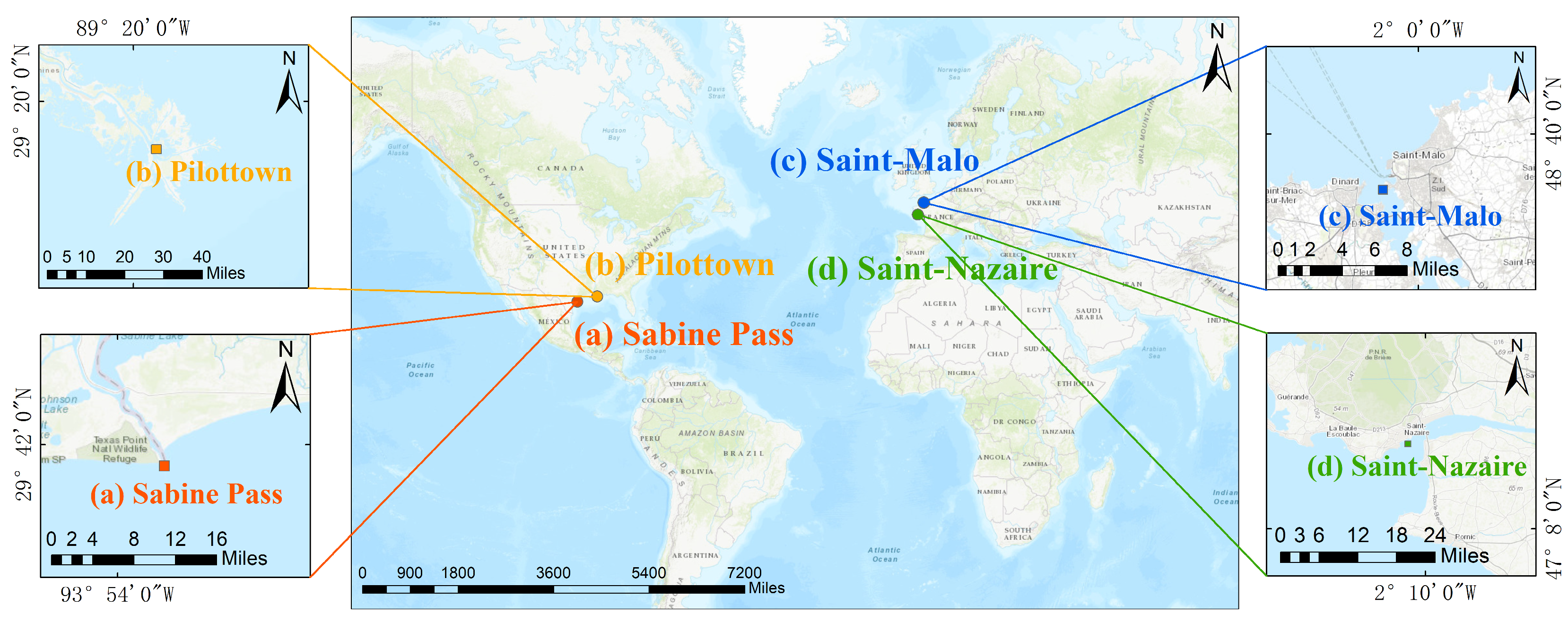
Figure 1. The location of the four tide gauge stations.
Jmse 13 01755 g001
Figure 2. Original water level data from the four tide gauge stations.
Jmse 13 01755 g002
Figure 3. Residual water level data from four tidal gauge stations.
Jmse 13 01755 g003
Figure 4. Experimental flowchart.
Jmse 13 01755 g004
Figure 5. Decomposition diagram of EEMD from the four tide gauge stations (a) Sabine Pass, (b) Pilottown, (c) Saint-Malo and (d) Saint-Nazaire.
Jmse 13 01755 g005
Figure 6. Decomposition diagram of VMD from the four tide gauge stations (a) Sabine Pass, (b) Pilottown, (c) Saint-Malo and (d) Saint-Nazaire.
Jmse 13 01755 g006
Figure 7. Frequency diagram of EEMD after FFT from the four tide gauge stations (a) Sabine Pass, (b) Pilottown, (c) Saint-Malo and (d) Saint-Nazaire.
Jmse 13 01755 g007
Figure 8. Frequency diagram of VMD after FFT from the four tide gauge stations (a) Sabine Pass, (b) Pilottown, (c) Saint-Malo and (d) Saint-Nazaire.
Jmse 13 01755 g008
Figure 9. Comparison of forecasted and true values for four tide gauge stations (a) Sabine Pass, (b) Pilottown, (c) Saint-Malo and (d) Saint-Nazaire over a month.
Jmse 13 01755 g009
Figure 10. Comparison of forecasted and true values for four tide gauge stations (a) Sabine Pass, (b) Pilottown, (c) Saint-Malo and (d) Saint-Nazaire over a week.
Jmse 13 01755 g010
Figure 11. Comparison of forecasted and true values for four tide gauge stations (a) Sabine Pass, (b) Pilottown, (c) Saint-Malo and (d) Saint-Nazaire over a day.
Jmse 13 01755 g011
Table 1. Forecast Accuracy of the Residual Water Levels at Each Station (cm).
Station NameTimeVMD-BPNNEEMD-BPNNBPNN
RMSEMAENSERMSEMAENSERMSEMAENSE
Sabine Passmonth2.952.220.93624.033.090.88105.534.340.7751
week2.251.903.382.864.884.22
day1.951.673.012.504.604.00
Pilottownmonth1.641.220.97101.861.490.96252.722.090.9199
week1.341.141.991.772.492.13
day0.920.761.731.611.751.44
Saint-Malomonth3.192.550.93585.234.250.82766.795.450.7096
week3.412.645.884.717.755.99
day3.272.706.174.967.826.45
Saint-Nazairemonth2.511.920.85573.863.070.65695.654.590.2660
week3.562.794.523.666.405.12
day1.211.004.453.804.113.43
Disclaimer/Publisher’s Note: The statements, opinions and data contained in all publications are solely those of the individual author(s) and contributor(s) and not of MDPI and/or the editor(s). MDPI and/or the editor(s) disclaim responsibility for any injury to people or property resulting from any ideas, methods, instructions or products referred to in the content.