Article

Artificial Texture-Free Measurement: A Graph Cuts-Based Stereo Vision for 3D Wave Reconstruction in Laboratory

College of Intelligent Systems Science and Engineering, Harbin Engineering University, Harbin 150001, China
*
Author to whom correspondence should be addressed.
J. Mar. Sci. Eng. 2025, 13(9), 1699; https://doi.org/10.3390/jmse13091699
Submission received: 27 July 2025 / Revised: 16 August 2025 / Accepted: 19 August 2025 / Published: 3 September 2025
(This article belongs to the Section Ocean Engineering)

Abstract

A novel method for three-dimensional (3D) wave reconstruction based on stereo vision is proposed to overcome the challenges of measuring water surfaces under laboratory conditions. Traditional methods, such as adding seed particles or projecting artificial textures, can solve the image problem caused by the optical properties of the water surface. However, these methods can be costly and complicated to operate. In this paper, the proposed method uses affine consistency as matching invariants, bypassing the need for artificial textures. The method presents new data and smoothness terms within the graph cuts framework to achieve robust wave reconstruction. In a laboratory tank experiment, the wave point clouds were successfully reconstructed using a binocular camera. The accuracy of the method was verified by comparing the reconstruction with theoretical values and the sequences of the wave probe.

1. Introduction

Measuring the spatial-temporal characteristics of wave is becoming increasingly important in marine and coastal engineering [1,2,3], with applications ranging from coastal protection design to offshore structure analysis. In laboratory conditions, measurements of wave surface in tanks are used as the basis for wave modeling studies. However, achieving accurate three-dimensional wave field measurements using stereo vision is fundamentally challenged by the transparent, reflective, and textureless nature of water surfaces. These optical properties make it difficult to establish correspondences between stereo image pairs, which is essential for depth reconstruction through triangulation. The development of imaging hardware and algorithms has led to increased attention from researchers towards measuring the three-dimensional (3D) wave field, which is considered a superior alternative to traditional single-point measurement means. Traditional methods for measuring 3D waves rely on deploying many single-point instruments, such as capacitive and resistive probes, in the water body to obtain instantaneous spatial measurements of waves. For instance, a study used multiple wave probes to acquire precise spatial-temporal data of waves at 1400 specific points [1]. The data were then synthesized to reconstruct the spatial-temporal wave field. However, measuring spatial wave fields using this method is complex and requires multiple repetitions of the experiment to acquire data for each wave condition. In addition, too many wave probes may interfere with the wave field itself. Therefore, it is essential to develop a solution capable of measuring three-dimensional spatial wave fields.
Non-intrusive sensors such as LiDAR and RGB-D cameras [4] typically measure distances based on the time-of-flight principle. In practice, the emission angle of the laser or structured light is strictly required. Additionally, this method may lead to measurement failures when the light is absorbed by transparent objects, especially for objects like waves in flumes or tanks. To improve the adaptability of the imaging system to the water environment and to ensure the photometric consistency of the images, some studies have used structured light-based techniques [5,6,7]. In contrast, stereo vision systems that use multiple cameras are more reliable and easier to use as they calculate depth using triangulation based on the correlation of image intensities. Zhu et al. project laser speckles onto the sand surface, but this method could not be used in the presence of significant waves [8]. Benetazzo et al. [9] proposed the WASS, a public pipeline that utilizes existing computer vision techniques. The pipeline employs feature matching algorithms (such as SIFT [10] and ORB [11]) to calibrate the binocular cameras, successfully reconstructing a large area of three-dimensional ocean waves [2,3,12]. However, observing a wave surface in a laboratory tank presents a significant challenge due to the lack of texture and the presence of curved specular reflection effects. Even if texture is present in some areas of the image, its reflection at different camera viewpoints can result in feature shifts and nonlinear deformations at the pixel level. To tackle this issue, mainstream methods have employed the strategy of introducing artificial textures into the observed scene. This type of schemes enhances the color or texture consistency of the image, thereby facilitating the accuracy of image matching and 3D reconstruction. The artificial textures are typically classified into two categories: particle seeding and projection patterns. Stereo matching or digital image correlation (DIC) is applied directly to the captured image, and the 3D reconstruction results are determined based on the principle of triangulation. Recent advances in stereo vision for fluid measurement have explored various approaches to address the transparency challenge. Machine learning-based methods have shown promise in feature extraction from water surfaces, though they require extensive training data [13,14]. Hybrid approaches combining multiple sensing modalities have been investigated [15,16], but they increase system complexity and cost. Our texture-free approach offers a simpler alternative that leverages geometric consistency rather than appearance-based matching.
The particle seeding methods involve selecting materials based on several factors, including image quality, uniform particle distribution on the water surface, and material degradability, to ensure both experiment feasibility and environmental sustainability. Gomit et al. [17] conducted an experiment to analyze waves generated by the passage of boats in a towing pond. They used polypropylene beads for this purpose but found that the material aggregated on the water surface. Caplier and his team [18] solved the problem of tracer material aggregation by using mineral particles of perlite. Ferreira et al. [19] used cork particles with a diameter of 1 mm as tracers, which provide better contrast with the untextured water surface and can be reused after drying to enhance the sustainability of the experiments. To enhance stereo matching accuracy, Fleming et al. [20] utilized millions of fluorescent flakes and developed specialized algorithms to precisely detect fluorescent features. Han et al. [21] used wax powder as seeds to measure flowing river water surface. Li et al. [22] used foam particles and optimized lighting to reconstruct 3D wave field, integrating threshold segmentation and stereo matching. Despite its effectiveness, the method struggles with particle clustering and displacement during intense fluctuations. To achieve a more stable texture in the wave field, researchers have projected regular patterns, such as python pattern, random patterns and grids, onto the water surface [23,24,25]. This type of method typically requires the use of specific opaque paint and light field settings.
Researchers are seeking more economical and easier-to-implement alternatives to adding artificial textures to experimental environments. This transition is reflected in the intensive study of experimental materials and repetition of experiments. As one of the solutions, researchers have investigated the contour information from the edges of the wave. Viriyakijja et al. [26] measured waves in a transparent tank and used edge detection to locate the edge information in the image. The edge information was triangulated to recover the two-dimensional waveform of the waves. Hernández et al. [27] measured the submerged portion of the vessel by binarizing the image to measure the water level, obtaining experimental data on 2D hydrodynamics. In [27], the blue dye was added to a glass flume to accurately obtain wave height information from binary images. Du et al. [28] developed an efficient algorithm for detecting fluid edges in a specific water surface scenario. Isidoro et al. measured the liquid level from the side of the glass flume to obtain the wave height [27]. Meanwhile, Douglas et al. [27] proposed a color segmentation-based approach to locate the water surface by examining the junction of the wave and trough using a lateral camera. The methods used in these efforts do not qualify as reconstructions based on stereo techniques because they rely on edge detection and area boundaries to recover wave contours and cannot reconstruct three-dimensional point clouds, i.e., the measurements obtained are limited to two-dimensional information. Furthermore, the side view perspective is only available from a glass flume, indicating limited applicability in varied experimental environments. However, the techniques of edge detection and water surface tracking can serve as inspiration. In recent years, the development of deep learning models, such as segment anything model (SAM) [29], has provided new possibilities for texture-free matching.
The main contributions of this study are as follows:
  • We use SAM (version 1.0) as a preprocessing step for water surface segmentation and replace the photometric or color consistency criterion in generalized stereo vision with the concept of affine consistency.
  • Within the framework of Graph Cuts, a global optimization algorithm [30] that has demonstrated superior accuracy and efficiency in computer vision [31,32,33,34], we introduce new data and smoothness terms based on affine consistency and superpixel boundary constraints, respectively.
  • Our approach operates solely at the software level and does not require any configurations or restrictions of the light field environment.
  • We present a proof of concept validated in controlled laboratory conditions, demonstrating the feasibility of texture-free 3D wave reconstruction with clearly identified limitations and future research directions.
The rest of this paper is organized as follows. Section 2 provides detailed mathematical derivations of the affine consistency criterion and its integration within the graph cuts framework. Section 3 presents the experimental results of the reconstructed wave and compares them quantitatively to the measurements obtained with the wave probe, including comprehensive sensitivity analysis and discussion of limitations. Finally, the conclusions and future work directions are given in Section 4.

2. Method

The binocular camera is a commonly used system for stereo vision measurements. After obtaining the correspondence, we can use the pre-calibrated intrinsic and extrinsic parameters of the camera model to recover the 3D points corresponding to the 2D pixels through the triangulation principle. The calibration parameters include the intrinsic parameters (focal length, principal point, and distortion coefficients) and extrinsic parameters (rotation and translation between cameras). These parameters are obtained using Zhang’s calibration method (implemented in OpenCV 4.5.0) with a checkerboard pattern, achieving a reprojection error of 0.1 pixels. The accuracy of these calibration parameters directly affects the triangulation precision and consequently the 3D reconstruction quality. We introduce a perturbation strategy based on graph cuts theory, specifically designed for fine matching of wave images that lack texture and exhibit specular reflections, which uses affine ratios as invariants. In this section, the first part explains affine consistency as a matching invariant for finding correspondences. The second part details the fine matching with perturbation based on graph cuts theory.

2.1. Affine Consistency as Matching Invariance

The affine consistency criterion is fundamental to our texture-free matching approach. We provide here a detailed mathematical derivation to clarify how affine ratios serve as robust matching invariants for water surfaces without artificial textures.
In [35], the epipolar lines are considered as the projection of line segments in three-dimensional space. Theoretically, affine ratio invariance only applies to planes. In stereo matching, it is considered acceptable to approximate local areas as the planar surfaces. This approximation is particularly valid for water surfaces in controlled laboratory conditions where wave slopes are moderate, as in our experiments with regular waves.
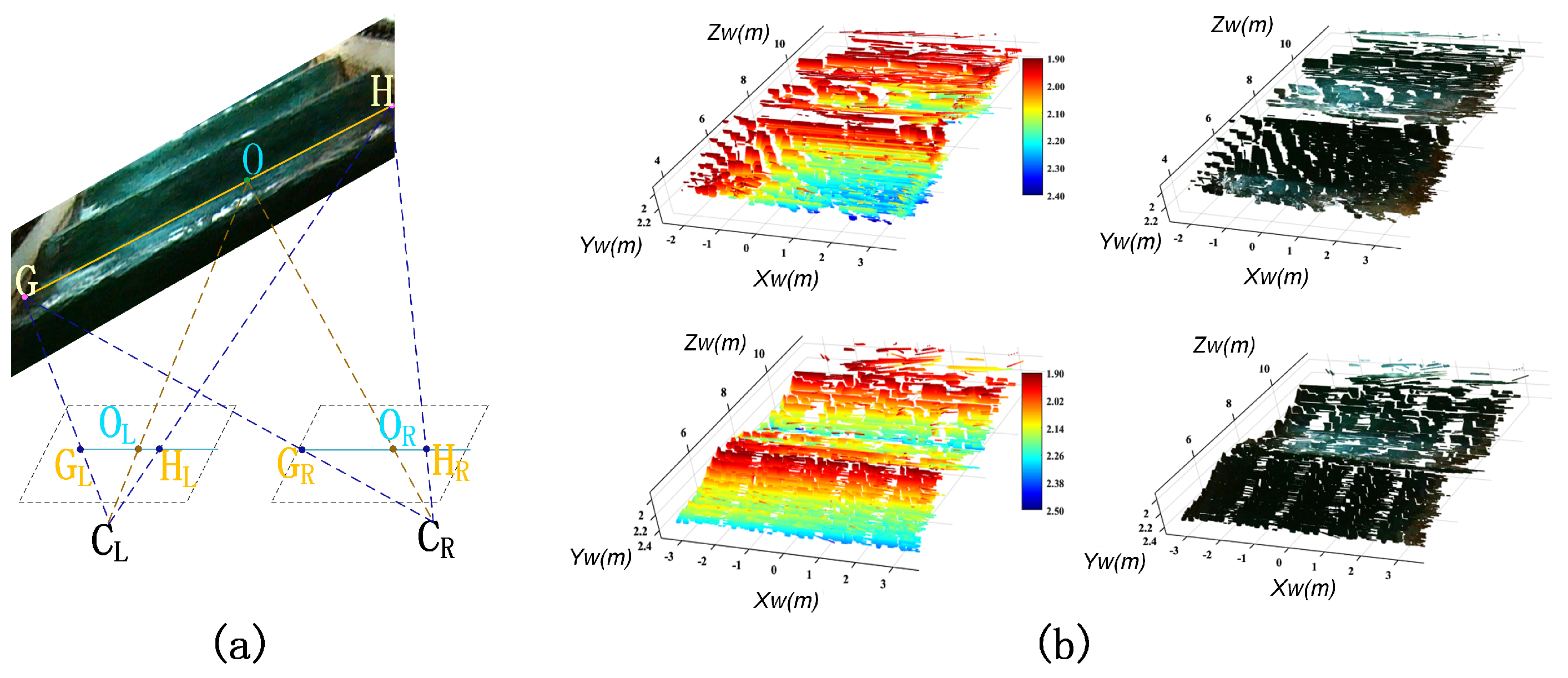
The mathematical foundation of affine invariance under perspective projection can be expressed as follows: Consider a 3D line segment with endpoints G and H , as well as any point O on this line. Under perspective projection to two camera views, the affine ratio is preserved:
| | H O | | | | O H | | = C
where C is the constant across views. This property holds because affine ratios are invariant under projective transformations when points are collinear.
In this study, the epipolar lines are aligned parallel to the horizontal axis of the image by epipolar constraints. The regions passed by an epipolar line in the left and right views corresponding to the relevant areas on the water surface in the three-dimensional world may not be strictly planar. However, if the optical axis is roughly aligned with the yaw direction of the wave tank, the proposed method can still follow the planar assumption, which is also relaxed due the smoothness term in this study.
The endpoints G and H of the epipolar line are chosen as the intersections of the epipolar line with semantic segmentation. These endpoints serve as the basis for computing affine consistency for the points that lie between them and through which the epipolar line passes. This study provides an example of SAM for water surface, as shown in Figure 1. To acquire the public field of view, we artificially set a region of interest (ROI) at one of the row indexes of the image. The ROI is selected to ensure overlap between the left and right camera views while excluding areas where water surface boundaries may be occluded or distorted by tank walls. Specifically, the ROI boundaries are determined by identifying the common visible area in both stereo views where the water surface segmentation can be reliably obtained, typically the central 80% of the overlapping field of view.
As shown in Figure 2a, the yellow line segments represent the epipolar lines within the segmented wave surface, with G and H being the determined endpoints located on this epipolar line, which are the projections of the endpoints of the line in R 3 space. The imaging coordinates of G and H within the left view are G L = [ x G L , y G L ] and H L = [ x H L , y H L ] , and G R = [ x G R , y G R ] , H R = [ x H R , y H R ] within the right view. The coordinates of any point O between the endpoints in the left and right views are O L = [ x O L , y O L ] and O R = [ x O R , y O R ] , respectively. The affine ratios used as the match invariance are
ρ O L = | | x G L x O L | | | | x O L x H L | | and ρ O R = | | x G R x O R | | | | x O R x H R | |
i.e., the Euclidean distance between ρ O L and ρ O R is used to measure the similarity between O L and O R .

2.2. Fine-Level Matching Framework with Perturbation

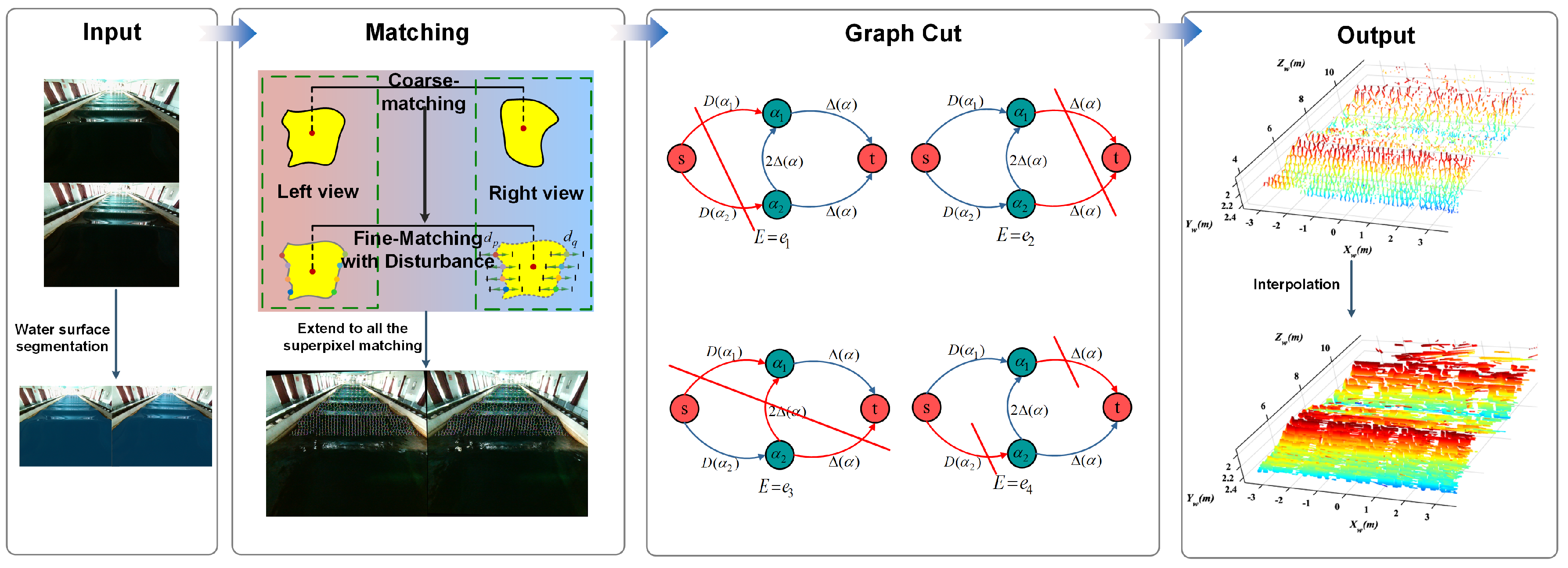
The complete algorithm pipeline consists of the following sequential steps: (1) Stereo image acquisition from calibrated cameras, (2) water surface segmentation using SAM to identify the region of interest, (3) epipolar line extraction based on calibration parameters, (4) superpixel boundary detection to identify matching primitives, (5) affine ratio calculation for correspondence candidates, (6) graph cuts optimization to determine optimal disparities, and (7) 3D point cloud generation through triangulation. Figure 3 illustrates this processing pipeline with the main computational stages.
Figure 2b shows the results of using our framework compared to direct matching techniques. The point clouds are colored to represent elevation mapping and water surface imagery. The proposed method demonstrates superior visual reconstruction quality and smoother performance. Therefore, while affine consistency can serve as a matching invariant, it cannot be directly applied in the matching process. Errors in direct matching methods arise from various factors, including the precision of semantic boundaries and the assumption of local planarity. Our improved matching framework utilizes a pair of intersections between the superpixel boundary and an epipolar line as the primitive matching unit, rather than individual pixels. The data term is based on affine invariance of epipolar line segments, while the smoothness is the preservation of superpixel boundaries. The proposed method finds the optimal affine correspondence of the superpixel boundary points in an energy-minimizing framework, which employs graph cuts theory and a perturbation strategy while integrating affine invariance and preserving the superpixel boundary.
The strategy of employing a pair of intersections, identified as points p and q, on an epipolar line is introduced to refine disparity calculations, as can be seen in Figure 1. The main process is illustrated in Figure 3: the primitive matching unit employed is the pair of boundary points located on an epipolar line within a superpixel. The initial disparity can be derived by estimating homography from feature correspondences outside the water surface within the image. Given a coarse disparity denoted as d, along with perturbation distances δ p and δ q for these endpoints, the final disparities are adjusted to d + δ p and d + δ q , respectively, within a predefined perturbation range δ p , q [ x m i n , x m a x ] . By designating pairs of points as the primitive matching units, the movement of each point is effectively constrained to maintain their left-right order and a certain spacing between them. Optimization is carried out for each individual superpixel. Upon obtaining the point cloud of superpixel boundary, the dense point cloud is generated through interpolation.
In the framework of graph cuts, both data and smoothness terms are utilized as weights for network edges. Decision-making nodes, namely the source and target, dictate the state of a network node, remaining unchanged when connected to the source and altering when linked to the target. The set A , consisting of potential bi-boundary points, embodies elements indicating node correspondences, defined as affinements a = ( p l , q l ; p r , q r ) , where p l corresponds to p r , and q l to q r . The state function f ( a ) determines the activity of a, inactive f ( a ) = 0 or active f ( a ) = 1 , with nodes categorized into two types: o for decisions on existing disparities and α for decisions on newly popped disparities. This design can identify the best disparities and discard those that are unstable, especially when the activities of both nodes are inactive.
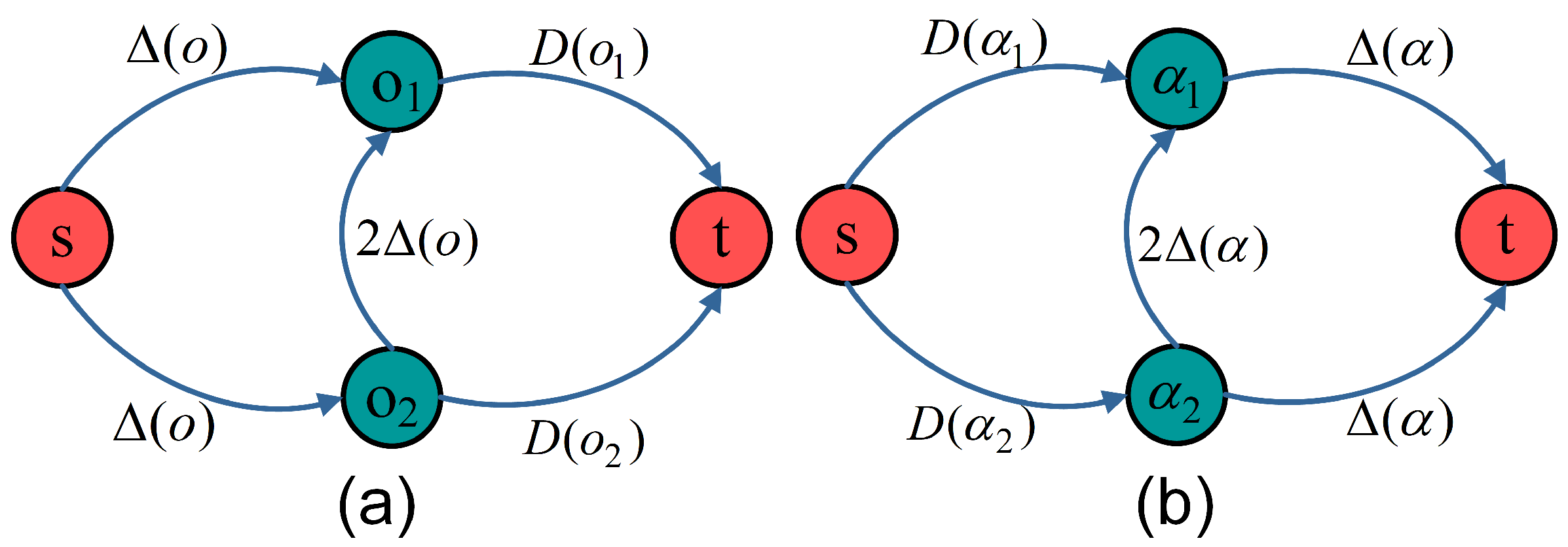
Specifically, α A represents decisions regarding newly popped disturbances ( δ p α , δ q α ) , with f ( α ) = 1 signifying the acceptance of the new disparity and f ( α ) = 0 rejection. In decision nodes o A o , regarding old disparities ( δ p o , δ q o ) not equal to the popped disturbances, the state f ( o ) = 1 indicates the retention of old disparities, while f ( o ) = 0 denotes the decision of disposal. The trigger function g ( · ) is capable of altering states f ( · ) , where g = 0 maintains the current state and g 0 triggers a state transition, mirroring the terminal nodes in graph cuts networks. A basic network without neighborhood smoothing constraints is shown in Figure 4a.
Then, we introduce the design of energy function and the analysis of edge weight deployment in network flow in detail. The energy function comprises data, smoothness, and exclusivity terms, i.e.,
E = E d a t a + E s m o o t h n e s s + E u n i q u e n e s s
It measures similarity, penalizes adjacent motion inconsistencies, and prevents conflicts between α and o nodes, respectively.
The data term is computed as
E d a t a = a , f ( a ) = 1 ( D ( a ) K )
where D ( a ) is the dissimilarity calculated by affine ratios, K is a constant, and it is set to the average of distances from the third smallest distance among affine ratio invariants for disturbances involving border points, adhering to a strategy derived from [36].
Using the consistency of the superpixel boundary as a smoothness constraint, the smoothness term is shown as
E s m o o t h n e s s = a 1 , a 2 Δ ( a ) · I ( f ( a 1 ) f ( a 2 ) )
where I ( f ( a 1 ) f ( a 2 ) ) indicates that the neighboring nodes have different states and Δ ( a ) is defined by
Δ ( a ) = λ 1 , if max ( | x i r x i 1 r | , | x i + 1 r x i r | ) < t λ 2 , otherwise
where λ is chosen to be proportional to K, following the strategy outlined in [31]. x i r represents the x-coordinate of the corresponding point in the ith row within the right view and t is a threshold for the difference between the neighboring points in a superpixel boundary. Small dissimilarities between neighboring nodes give a greater value of the smoothness term, while large dissimilarities give a lower value. The complete network flow with smoothness terms is shown in Figure 5.
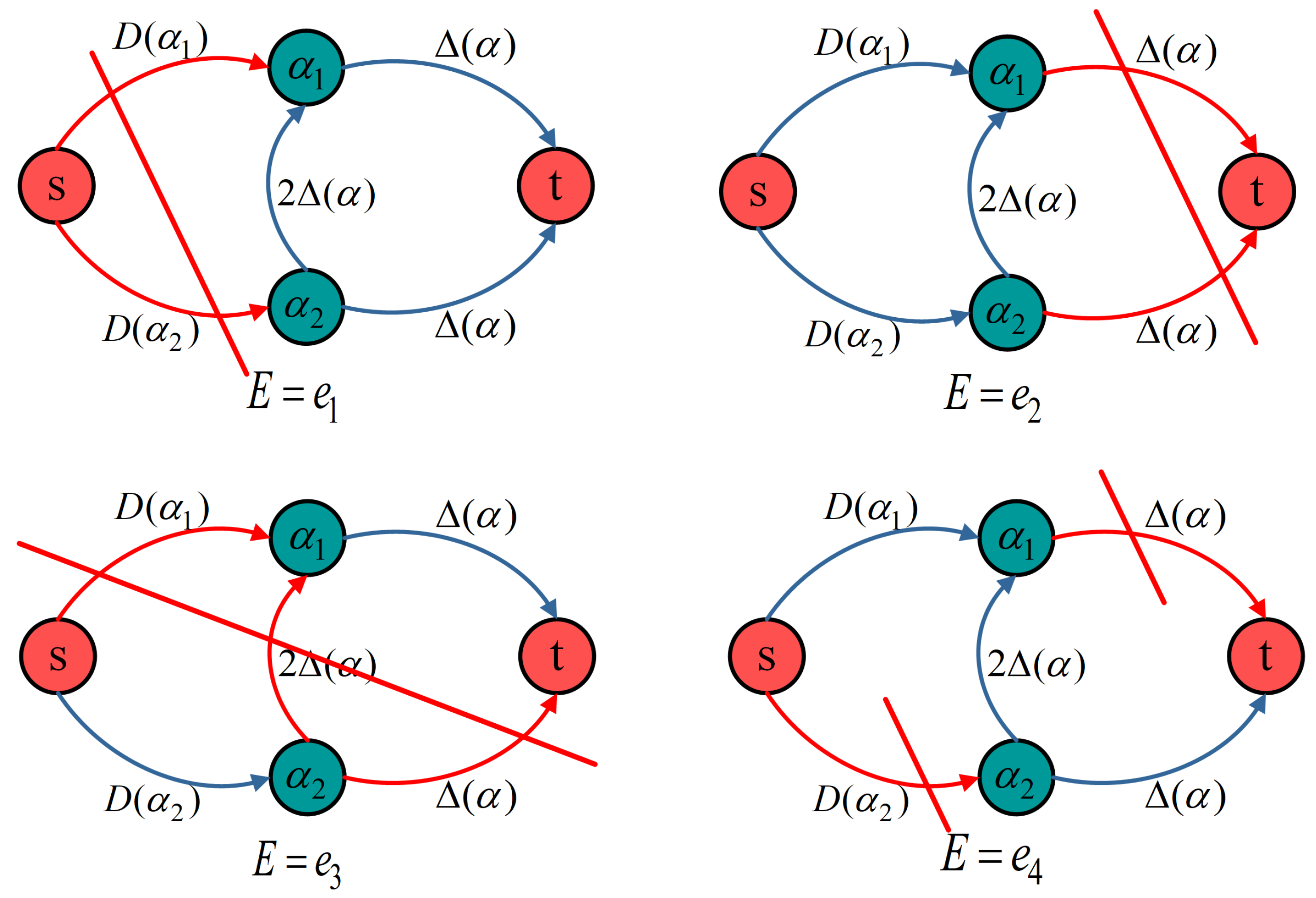
To explain the placement of edge weights, we analyze the smoothness term using α as an example. Specifically, we consider four cut costs, as can be seen below.
e 1 = D ( α 1 ) + D ( α 2 ) e 2 = Δ ( α 1 ) + Δ ( α 2 ) = 0 e 3 = D ( α 1 ) + Δ ( α 1 ) e 4 = D ( α 2 ) + Δ ( α 2 )
When e 1 is the minimum energy, the segmentation result is g ( α 1 ) = 1 , g ( α 2 ) = 1 , requiring either Δ ( α 1 ) > | D ( α 1 ) | or Δ ( α 2 ) > | D ( α 2 ) | . When e 2 is the minimum energy, the segmentation result is g ( α 1 ) = 0 and g ( α 2 ) = 0 , requiring either Δ ( α 1 ) < | D ( α 1 ) | or Δ ( α 2 ) < | D ( α 2 ) | . When e 3 is the minimum energy, the segmentation result is g ( α 1 ) = 1 and g ( α 2 ) = 0 , requiring both D ( α 2 ) D ( α 1 ) > 0 ( Δ ( α 1 ) + Δ ( α 2 ) ) and Δ ( α 1 ) < | D ( α 1 ) | . When e 4 is the minimum energy, the segmentation result is g ( α 1 ) = 0 and g ( α 2 ) = 1 , requiring D ( α 1 ) D ( α 2 ) > 0 ( Δ ( α 1 ) + Δ ( α 2 ) ) . The four types of cuts are detailed in Figure 6.
The decision-making cases are summarized in Table 1. To ensure accurate determination of the optimized perturbation, it is important to avoid any conflict in decision-making between the o node and the α node regarding the perturbation parameters. For example, in Case 2, the decision is to keep ( d p o , d q o ) while accepting ( d p α , d q α ) . To address this issue, we introduce a uniqueness term in the energy function and adjust the network configuration accordingly, as shown in Figure 4b. In such cases, the trigger function g ( · ) is considered illegal if it satisfies both g ( o ) = 0 and g ( α ) = 1 . With the network design in Figure 4b, when minimizing cost cuts, zero-weight edges are given priority for cutting. Therefore, the decision involves choosing to cut either the edge connected to terminal node or the one connected to terminal node, ensuring that g ( o ) = 0 and g ( α ) = 1 never occur simultaneously, thereby preventing conflicting decisions. The uniqueness term can be expressed as
E u n i q u e n e s s = a 1 A o , a 2 A α · I ( g ( a 1 ) = 0 , g ( a 2 ) = 1 )
The proposed perturbation strategy is outlined in Algorithm 1 based on the framework of graph cuts.
Algorithm 1 The iteration of the perturbation strategy in the graph cuts.
Input: The sparse pairs of boundary points within a superpixel; a coarse disparity d; a perturbation range [ d m i n , d m a x ] ; number of loops N.
Output: All the final disparity ( d + δ p i , d + δ q i ) within a superpixel.
Initialization:  E o p t m = E i n i t i a l , make [ d m i n , d m a x ] in a random order, set the map of the perturbations M p e r t u r b a t i o n s .

While  n < N :
   For each  δ p , δ q [ d m i n , d m a x ] :
      Build the graph cuts network G ( o , α )
      For each  a = ( p l , q l ; p r , q r ) :
          d a n e w = d + δ p + δ q , d o l d = M p e r t u r b a t i o n s
         Calculate data E ( a ) and smoothness E ( a ) by (3) and (4)
         Add the edge weights and uniqueness E ( a ) to the network G ( o , α )
      End for
      Compute the minimal cost E n e w of G ( o , α )
      If  E n e w < E o p t m :
          E o p t m = E n e w
         Update M p e r t u r b a t i o n s based the decisions of G ( o , α )
         Done[:] = False
      Else:
         Done[ ( δ p , δ q ) ] = True
   End for
   If Done[:] == True:
      Return perturbations of all boundary pairs
End while

3. Experiment

3.1. Experimental Setup

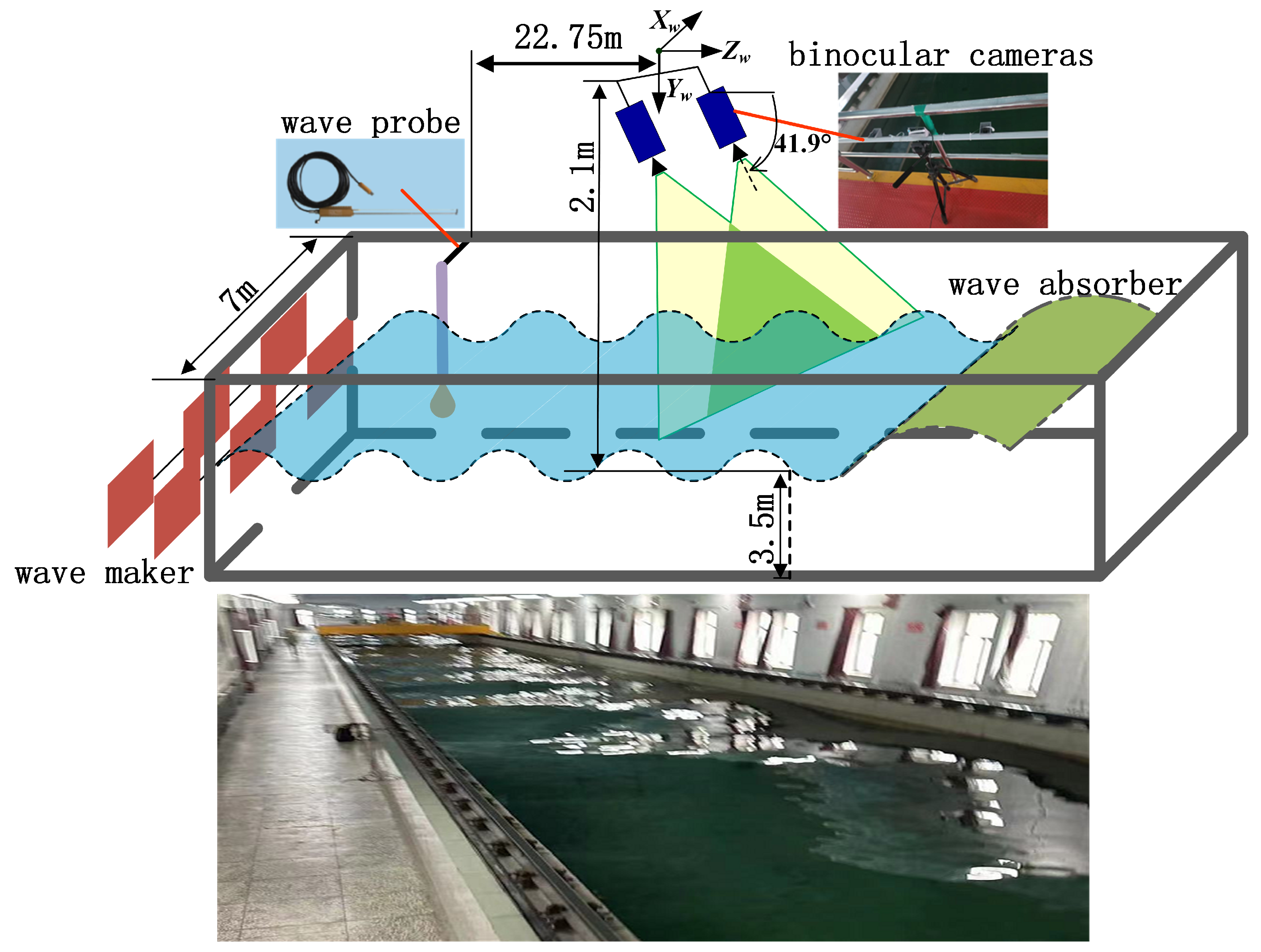
The experimental wave tank (TS18900, Edinburgh Designs, Edinburgh, UK) has dimensions of 108 m in length, 7 m in width, and 3.5 m in depth, and is equipped with a paddle-type wave generator and passive wave dampers. A low-cost binocular camera (RYS-800WAF, Rongyangsheng Electronic Technology Co., Ltd., Shenzhen, China) is used in the experiment, which is fixed on a tripod after calibration. The camera is located 2.1 m above the static water surface, with its baseline parallel to the lateral direction of the tank. The optical axis of the camera forms a 41.9-degree angle with the calm water surface in the Z w direction, as shown in Figure 7. The camera is calibrated using Zhang’s calibration method [33], resulting in a reprojection error of 0.1 pixels. A wave height probe, perpendicular to the static water surface, is placed at a certain location in the tank. Given the distance between the probe and the camera, as well as the wavelength and period of the waves, it is possible to synchronize the timestamps of the two measuring instruments.
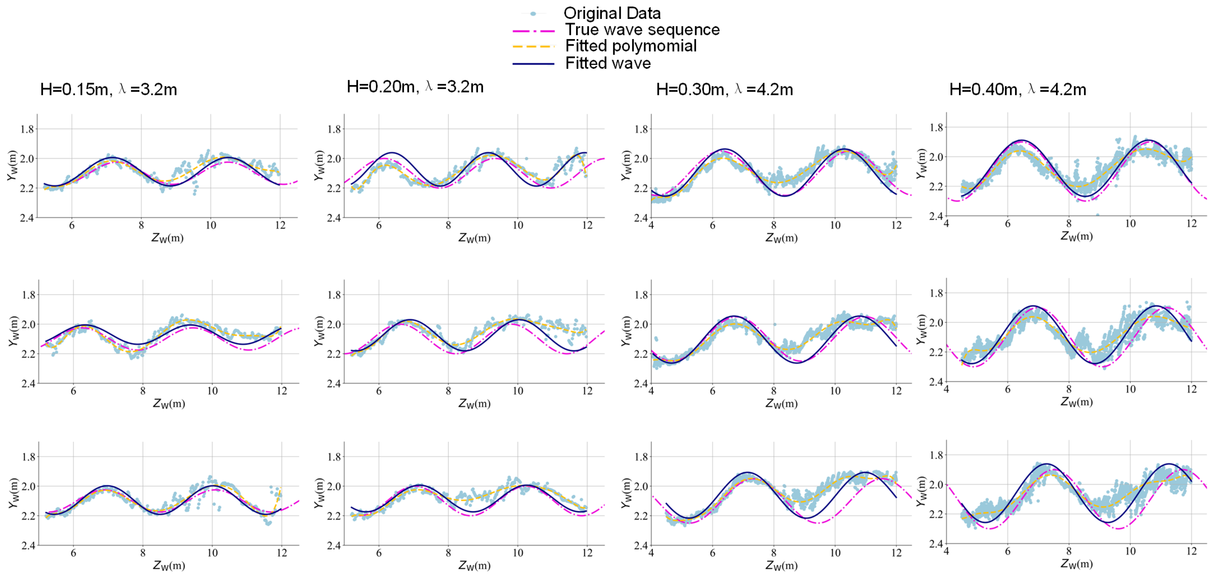
By setting a predetermined angle, the reconstructed 3D point cloud of the wave can be transformed from the camera coordinate system to the world coordinate system. The static water surface and instantaneous elevations are obtained from the YZ cross-section of the wave. In the Z w direction, a resolution of 0.01 m is set, meaning that for every 0.01 m of point cloud in the Z w direction, we calculate its average, as illustrated in Figure 8.

3.2. Experimental Results

To evaluate the feasibility and stability of the proposed 3D wave reconstruction method, experiments were conducted on waves with varying parameters. The image segmentation results revealed that wave height influences the clarity of segmentation boundaries. Hence, we focused more on examining the impact of distinguishable wave heights on method accuracy. In this simulation, four waves were simulated with four different wave heights and two wavelengths, each lasting approximately 60 s. The experimental scenarios were selected to test the method across a range of wave conditions typical in laboratory wave studies. The four wave heights (0.15 m, 0.20 m, 0.30 m, 0.40 m) and two wavelengths (3.2 m, 4.2 m) represent regular waves from small to moderate amplitudes, allowing us to evaluate the method’s performance as wave steepness increases. These parameters were chosen to remain within the linear wave regime while providing sufficient variation to assess reconstruction accuracy. The 60 s duration ensures statistical stability in the measurements.
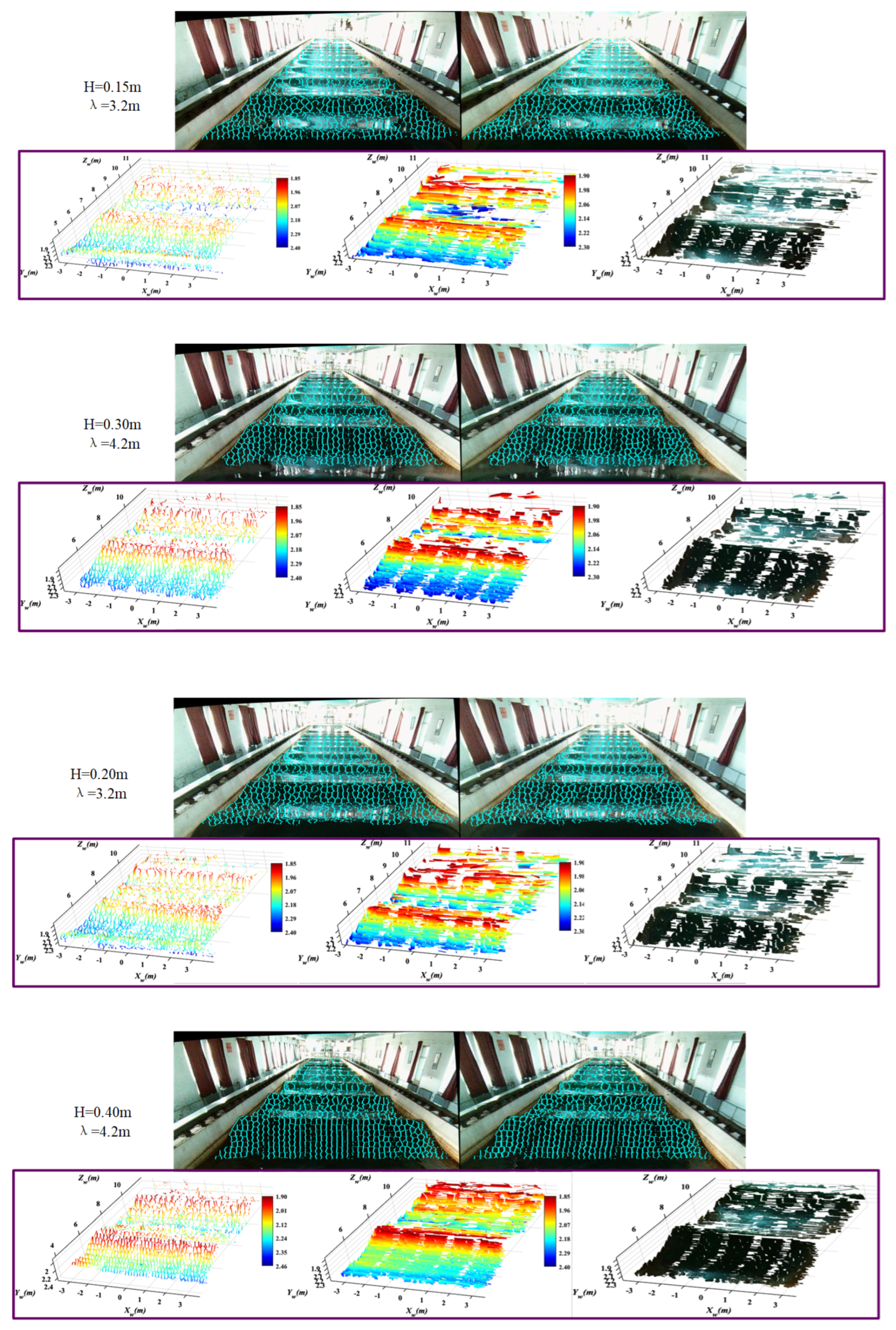
As shown in Figure 9, we present the 3D reconstruction results of the wave under four conditions in the form of point clouds. It is clearly visible from the figure that the quality of the reconstruction decreases as the point cloud moves away from the camera. After acquiring the initial wave point cloud, we need to transform it from the camera coordinate system to the world coordinate system, with the transformation matrix as demonstrated below:
X w Y w Z w = 1 0 0 0 cos β sin β 0 sin β cos β X c Y c Z c
where [ X w , Y w , Z w ] T are the 3D coordinates under the world coordinate system, [ X c , Y c , Z c ] T are the 3D coordinates under the camera coordinate system, and β is the angle at which the camera coordinate system is rotated counterclockwise around the X-axis to the world coordinate system.
In Equation (7), the transformation matrix uses a single rotation angle β around the X-axis because our experimental setup was specifically designed with the camera baseline aligned parallel to the tank’s lateral direction. This configuration requires only one rotation to align the camera coordinate system with the world coordinate system. The angle β represents the tilt angle between the camera’s optical axis and the horizontal plane. For more general camera orientations, a full rotation matrix R = R z ( γ ) R y ( α ) R x ( β ) with three Euler angles is required, where γ , α , and β represent rotations around the Z, Y, and X axes, respectively.
To better observe the spatial-temporal characteristics of the wave field measurements, we selected three frames, one frame apart, in each working condition for waveform fitting analysis of the discrete heights. As illustrated in Figure 8, using slicing operations allows direct observation of the error between the measured values and the true values recorded by the probe. The points representing the wave elevation are continuous and smooth, yet beyond 9 m in Z w , the consistency of the discrete points with the true waveform (the pink curve) deteriorates. To enable a quantitative comparison between the parameters of the discrete data and the true values, it is necessary to reconstruct waveforms from the discrete elevation points.
High-degree polynomials were employed to fit the discrete points. Subsequently, an error function was obtained using the existing polynomial and a cosine wave to be fitted, i.e.,
e ( A , B , C , D ) = i ( A · cos ( B x i + C ) + D n = 0 8 a n x i n )
where ( A , B , C , D ) are the amplitude, frequency, phase shift, and elevation shift of the trigonometric function, respectively, and n = 0 8 a n x n is a 9th degree polynomial. The parameters of the trigonometric function were obtained through error minimization.
The waveform recovery strategy allows to obtain optimal waveform estimates in the instantaneous spatial domain based on the discrete elevation points of the frame, using the global wave sequence in the field of camera view. The direction of propagation in the recovered waveforms, as estimated from successive multiple frames, is consistent with the experimental setup, i.e., forward along Z w . The waveforms were quantitatively analyzed to assess the accuracy and robustness of the proposed method, as shown in Table 2 and Table 3.
Table 2 and Table 3 demonstrate the accuracy of quantitative measurements for the elevation and wavelength of the wave. The measurements were estimated through the image frames represented in Figure 8, and R 2 metric was calculated for whole wave and half-wave at a point cloud reconstructed from a frame. The R 2 metric is provided as
R 2 = 1 i = 1 N ( y i t y i m ) 2 i = 1 N ( y i t y ¯ t ) 2
where y i t and y i m are the theoretical and measured values of the elevation of the ith point, respectively, and y ¯ t is the mean of the true values.
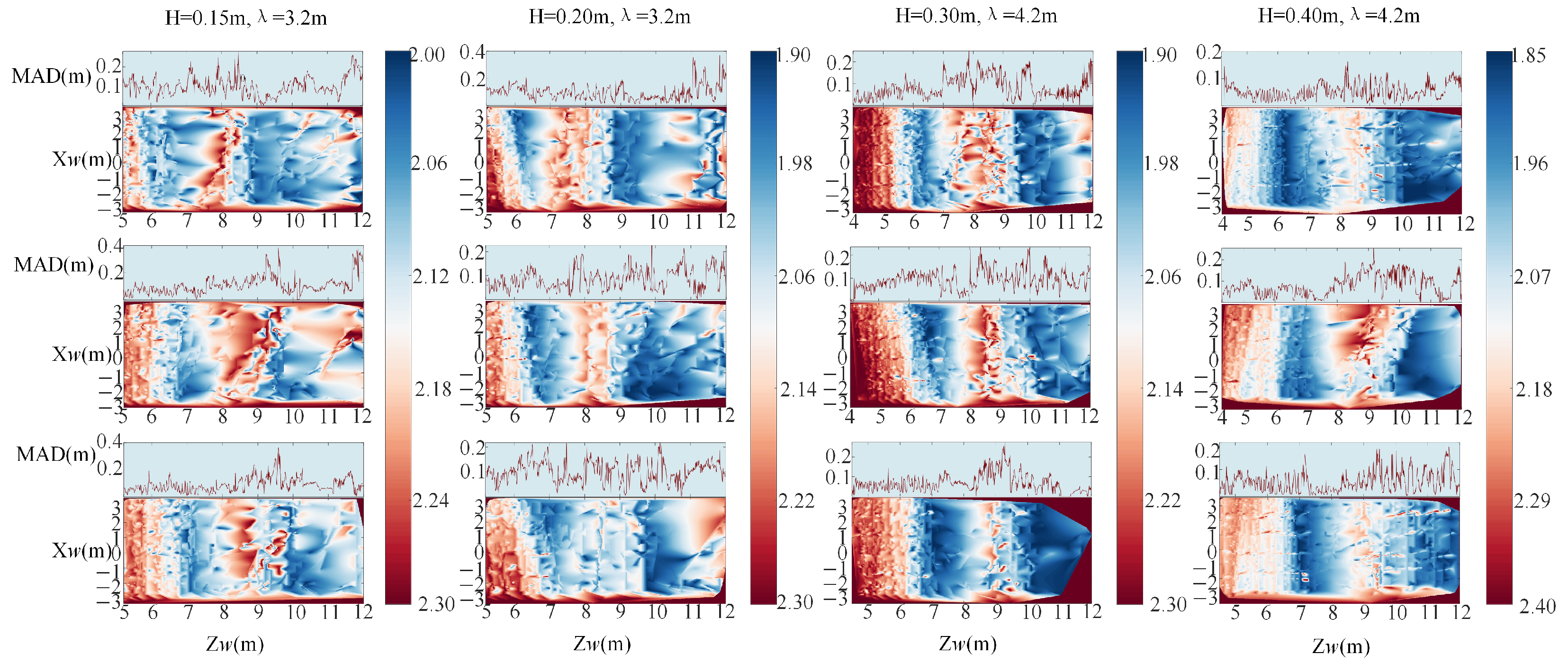
Figure 10 illustrates the elevation data in the XZ-plane. The Mean Absolute Deviation (MAD) is calculated for elevation values that share the same Z-coordinate but vary with the X-axis, forming a curve along Z w . The figure demonstrates that within the Z w , the MAD is under 0.1 m in the first half of the XZ-plane and around 0.2 m in the second half for the four different wave conditions. As the waveform moves away from the camera along the Z w direction, its imaging quality and the clarity of the segmentation boundaries deteriorate.

3.3. Parameter Selection and Theoretical Justification

The selection of key parameters in our method requires careful consideration based on theoretical principles and the characteristics of the wave measurement problem. We provide here the rationale for our parameter choices and discuss their expected impact on reconstruction performance.
The parameter K, which represents the threshold in the data term calculation, plays a crucial role in the optimization process. As stated in our methodology, K is set as the average of distances from the third smallest distance among affine ratio invariants for disturbances involving border points. This statistical approach balances between being robust to outliers (unlike using the minimum distance) and maintaining sensitivity to valid matches. While comprehensive sensitivity analysis requires systematic variation of K across different scales, this choice of a robust statistical measure should theoretically provide stable performance across different wave conditions.
The resolution parameter of 0.01 m for Z-direction averaging is selected based on the expected wave characteristics and measurement precision. This value represents approximately 1/320 of the shortest wavelength (3.2 m) in our experiments, which satisfies the Nyquist sampling criterion for accurate wave reconstruction. Theoretically, finer resolutions would amplify measurement noise without adding meaningful information, while coarser resolutions would lose important wave features.
The choice of a 9th-degree polynomial for waveform fitting is determined through preliminary tests with our wave data. This degree provides sufficient flexibility to represent the sinusoidal wave shapes while avoiding the numerical instabilities associated with higher-degree polynomials. The selection aligns with the principle that the polynomial degree should be high enough to capture the wave form but low enough to maintain numerical stability and avoid overfitting.

3.4. Limitations and Scope

It is important to acknowledge the limitations of our current work to provide a transparent assessment of the method’s applicability. Our experimental validation was conducted in a single laboratory setup with a fixed camera configuration where the baseline was parallel to the tank’s lateral direction. The experiments were performed under controlled lighting conditions with clear water and regular waves generated by a paddle-type wavemaker. This controlled environment, while essential for initial validation, limits our ability to claim broader generalizability without additional testing in diverse conditions.
The method’s performance boundaries become apparent when considering more complex wave patterns. Our experiments were limited to regular waves with the wave heights and wavelengths specified in Table 2 and Table 3. The fundamental assumption of surface continuity that underlies our affine consistency approach would be violated in breaking waves where the surface topology becomes discontinuous. Similarly, the method has not been validated for multi-directional wave fields or highly turbulent surfaces with foam and whitecapping, which would pose significant challenges for the segmentation process.
As evident from the results presented in Figure 10, reconstruction quality exhibits spatial variation within the measurement volume. The performance degradation with increasing distance from the camera can be attributed to several factors. The reduction in effective image resolution at far distances directly impacts the precision of feature localization. Additionally, the segmentation boundaries become less reliable as the apparent size of the water surface in the image decreases. These factors combine to produce accumulated errors in the affine ratio calculations, resulting in the observed decrease in reconstruction accuracy in the far field.

3.5. Discussion

Figure 8 illustrates the consistency between the measured waveforms fitted using the reconstructed points and the sequences given by the wave probe. In all cases, the measured wavelengths and elevations are generally consistent with the values of the wave probe. The phase difference is larger for the case with a wavelength of 4.2 m due to the error introduced by the corresponding larger wave speed. In Table 2 and Table 3, the R 2 metrics is generally twice as high for the first half of the waveforms (5 to 8.5 m in the Z w direction) compared to the overall waveforms (5 to 12 m in the Z w direction) for all cases. Similar to the R 2 metric, the MAD in Figure 10 also performs better in the first half of the range. This is because the quality of semantic segmentation decreases and the scale becomes smaller as the water surface moves further away from the camera, resulting in reduced distinguishability of the affine invariance. For wave elevation measurements with a theoretical height of 0.4 m, the maximum error does not exceed 3%, indicating satisfactory estimation performance, particularly without using artificial surface textures to aid measurement.
Errors can occur during the waveform fitting process and the stereo measurement system. The metrics being compared are derived from regular waves that are fitted from discrete measurement points, such as the wavelengths and wave heights. The fitting process minimizes an error objective function between a trigonometric and a polynomial. However, outliers in the discrete points of wave height can lead to significant deviations between the fitting results and the theoretical values. Additionally, the quantization error of the discrete pixels in the sensor is also a source of error. Finally, imaging noise and pixel dispersion can affect the identification of automatic segmentation boundaries. The affine consistency is highly dependent on the accuracy of the boundaries. However, the smoothness term based on the boundary constraint of superpixel allows us to relax the accuracy requirements of the segmentation boundaries, making it an alternative to photometric consistency.
In stereo vision systems, specular reflections make it impossible to directly match the patterns and textures of an object across the stereo image pairs. This study leverages superpixel boundaries as basic matching primitives to establish correspondences, effectively addressing the challenges posed by specular reflection. The technique not only identifies areas affected by specular reflectivity, but also infers the exact correspondence of textures in one view within another, assuming the absence of specular reflectivity. In fact, this mapping process is equivalent to the simulation of Lambertian surface imaging in binocular vision system.

4. Conclusions and Future Work

This paper proposes a graph cuts-based method for 3D wave reconstruction of a laboratory tank without artificial patterns or textures. By generating regular waves in a tank using a wavemaker, we compared the reconstructed 3D wave with sequences measured by a wave probe and the theoretical values to assess the proposed method. In this study, we used affine consistency instead of photometric consistency as the matching invariant and proposed a novel smoothness term based on the motion consistency of the superpixel boundary. We successfully integrated the affine matching invariant and smoothness term into the graph cuts algorithm for energy minimization.
Our experimental results demonstrate that the method can achieve wavelength measurement errors of 1.12–8.28% and wave height errors of 3.17–11.60% in controlled laboratory conditions. The method performs best in the near-field (5–8.5 m from camera) with R2 values reaching 0.95 for optimal conditions. However, we acknowledge that this work represents a proof of concept validated in a single experimental setup, and several limitations must be addressed for broader applicability.
The proposed method can achieve high consistency with measurements obtained by the wave probe within a certain field of frame view. It effectively addresses the challenges of textureless and specular reflections on wave surfaces in the laboratory, without relying on artificial textures or elaborate light fields. The optimization process is performed on individual superpixels, each of which provides a boundary constraint. The independence of the superpixels allows for parallel processing potential of the method.

Future Work

The current work establishes a foundation for texture-free wave reconstruction, but several important research directions remain to be explored. The most immediate priority is to extend the validation to diverse experimental setups with different camera configurations, tank geometries, and wave generation systems. Such extended validation would help establish the generalizability of the affine consistency principle across various laboratory conditions and identify any setup-specific adaptations that may be required.
The method’s extension to more complex wave patterns presents both theoretical and practical challenges. Breaking waves, irregular waves, and multi-directional wave fields requires fundamental adaptations to the current approach. The surface continuity assumption that underlies our method needs to be relaxed or reformulated for breaking waves. Advanced segmentation strategies, possibly leveraging recent developments in deep learning models, could help handle the more complex boundaries present in turbulent or foam-covered surfaces.
For real-world deployment beyond laboratory settings, the method requires substantial enhancements to handle varying natural lighting conditions, surface contamination, and environmental disturbances. The development of adaptive algorithms that can adjust to changing illumination and the integration with weather-resistant hardware systems is essential steps toward field applications. Additionally, exploring hybrid approaches that combine our texture-free method with minimal artificial enhancements could provide a practical path forward for particularly challenging conditions.
Performance optimization represents another crucial area for development. The current processing speed limits real-time applications, but GPU acceleration and optimized implementations of the graph cuts algorithm could potentially achieve the necessary throughput for dynamic wave monitoring applications. This work provides a proof of concept that texture-free wave measurement is feasible and could significantly simplify experimental procedures in hydraulic laboratories while maintaining acceptable accuracy for many applications.

Author Contributions

Conceptualization, F.W. and Q.Z.; methodology, F.W.; software, F.W.; validation, F.W. and Q.Z.; formal analysis, F.W.; investigation, F.W.; resources, Q.Z.; data curation, F.W.; writing—original draft preparation, F.W.; writing—review and editing, F.W. and Q.Z.; visualization, F.W.; supervision, Q.Z.; project administration, Q.Z.; funding acquisition, Q.Z. All authors have read and agreed to the published version of the manuscript.

Funding

This research was funded by the National Natural Science Foundation of China Grant No. 52171299.

Data Availability Statement

The data presented in this study are available on request from the corresponding author.

Conflicts of Interest

The authors declare no conflicts of interest.

References

  1. Swan, C.; Sheikh, R. The interaction between steep waves and a surface-piercing column. Phil. Trans. R. Soc. A 2015, 373, 20140114. [Google Scholar] [CrossRef]
  2. Douglas, S.; Cornett, A.; Nistor, I. Image-based measurement of wave interactions with rubble mound breakwaters. J. Mar. Sci. Eng. 2020, 8, 472. [Google Scholar] [CrossRef]
  3. Mou, T.; Shen, Z.; Xue, G. Task-driven learning downsampling network based phase-resolved wave fields reconstruction with remote optical observations. J. Mar. Sci. Eng. 2024, 12, 1082. [Google Scholar] [CrossRef]
  4. Pan, Z.; Hou, J.; Yu, L. Optimization RGB-D 3D reconstruction algorithm based on dynamic SLAM. IEEE Trans. Instrum. Meas. 2023, 72, 5008413. [Google Scholar] [CrossRef]
  5. Zhou, P.; Cheng, Y.; Zhu, J.; Hu, J. High-dynamic-range 3D shape measurement with adaptive speckle projection through segmentation-based mapping. IEEE Trans. Instrum. Meas. 2022, 72, 5003512. [Google Scholar]
  6. Ou, Y.; Fan, J.; Zhou, C.; Tian, S.; Cheng, L.; Tan, M. Binocular structured light 3D reconstruction system for low-light underwater environments: Design, modeling, and laser-based calibration. IEEE Trans. Instrum. Meas. 2023, 72, 5010314. [Google Scholar] [CrossRef]
  7. Hu, Y.; Rao, W.; Qi, L.; Dong, J.; Cai, J.; Fan, H. A refractive stereo structured-light 3D measurement system for immersed object. IEEE Trans. Instrum. Meas. 2022, 72, 5003613. [Google Scholar]
  8. Zhu, S.; Liu, J.; Guo, A.; Li, H. Non-contact measurement method for reconstructing three-dimensional scour depth field based on binocular vision technology in laboratory. Measurement 2022, 200, 111556. [Google Scholar] [CrossRef]
  9. Bergamasco, F.; Torsello, A.; Sclavo, M.; Barbariol, F.; Benetazzo, A. WASS: An open-source pipeline for 3D stereo reconstruction of ocean waves. Comput. Geosci. 2017, 107, 28–36. [Google Scholar] [CrossRef]
  10. Lowe, D.G. Distinctive image features from scale-invariant keypoints. Int. J. Comput. Vision 2004, 60, 91–110. [Google Scholar] [CrossRef]
  11. Rublee, E.; Rabaud, V.; Konolige, K.; Bradski, G. ORB: An efficient alternative to SIFT or SURF. In Proceedings of the IEEE International Conference on Computer Vision, Barcelona, Spain, 6–13 November 2011; pp. 2564–2571. [Google Scholar]
  12. Wolrige, S.H.; Howe, D.; Majidiyan, H. Intelligent computerized video analysis for automated data extraction in wave structure interaction; a wave basin case study. J. Mar. Sci. Eng. 2025, 13, 617. [Google Scholar] [CrossRef]
  13. Sun, D.; Gao, G.; Huang, L.; Liu, Y.; Liu, D. Extraction of water bodies from high-resolution remote sensing imagery based on a deep semantic segmentation network. Sci. Rep. 2024, 14, 14604. [Google Scholar] [CrossRef]
  14. Wang, Z.; Gao, X.; Zhang, Y. HA-Net: A lake water body extraction network based on hybrid-scale attention and transfer learning. Remote Sens. 2021, 13, 4121. [Google Scholar] [CrossRef]
  15. Fitzpatrick, A.; Mathews, R.P.; Singhvi, A.; Arbabian, A. Multi-modal sensor fusion towards three-dimensional airborne sonar imaging in hydrodynamic conditions. Commun. Eng. 2023, 2, 16. [Google Scholar] [CrossRef]
  16. Wang, F.; Zhu, Q.; Cai, C.; Wang, X.; Qiao, R. From points to waves: Fast ocean wave spatial–temporal fields estimation using ensemble transform Kalman filter with optical measurement. Coast. Eng. 2025, 197, 104690. [Google Scholar] [CrossRef]
  17. Gomit, G.; Chatellier, L.; Calluaud, D.; David, L.; Fréchou, D.; Boucheron, R.; Perelman, O.; Hubert, C. Large-scale free surface measurement for the analysis of ship waves in a towing tank. Exp. Fluids 2015, 56, 184. [Google Scholar] [CrossRef]
  18. Caplier, C.; Rousseaux, G.; Calluaud, D.; David, L. Energy distribution in shallow water ship wakes from a spectral analysis of the wave field. Phys. Fluids 2016, 28, 107104. [Google Scholar] [CrossRef]
  19. Ferreira, E.; Chandler, J.; Wackrow, R.; Shiono, K. Automated extraction of free surface topography using SfM-MVS photogrammetry. Flow Meas. Instrum. 2017, 54, 243–249. [Google Scholar] [CrossRef]
  20. Fleming, A.; Winship, B.; Macfarlane, G. Application of photogrammetry for spatial free surface elevation and velocity measurement in wave flumes. Pro. IMechE 2019, 233, 905–917. [Google Scholar] [CrossRef]
  21. Han, B.; Endreny, T.A. River surface water topography mapping at sub-millimeter resolution and precision with close range photogrammetry: Laboratory scale application. IEEE J. Sel. Top. Appl. Earth Obs. Remote Sens. 2014, 7, 602–608. [Google Scholar] [CrossRef]
  22. Li, D.; Xiao, L.; Wei, H.; Li, J.; Liu, M. Spatial-temporal measurement of waves in laboratory based on binocular stereo vision and image processing. Coastal Eng. 2022, 177, 104200. [Google Scholar] [CrossRef]
  23. van Meerkerk, M.; Poelma, C.; Westerweel, J. Scanning stereo-PLIF method for free surface measurements in large 3D domains. Exp. Fluids 2020, 61, 19. [Google Scholar] [CrossRef]
  24. Bung, D.B.; Crookston, B.M.; Valero, D. Turbulent free-surface monitoring with an RGB-D sensor: The hydraulic jump case. J. Hydraul. Res. 2021, 59, 779–790. [Google Scholar] [CrossRef]
  25. Evers, F.M. Videometric water surface tracking of spatial impulse wave propagation. J. Vis. 2018, 21, 903–907. [Google Scholar] [CrossRef]
  26. Viriyakijja, K.; Chinnarasri, C. Wave flume measurement using image analysis. Aquat. Procedia 2015, 4, 522–531. [Google Scholar] [CrossRef]
  27. Hernández, I.D.; Hernández-Fontes, J.V.; Vitola, M.A.; Silva, M.C.; Esperança, P.T. Water elevation measurements using binary image analysis for 2D hydrodynamic experiments. Ocean Eng. 2018, 157, 325–338. [Google Scholar] [CrossRef]
  28. Du, H.; Li, M.; Meng, J. Study of fluid edge detection and tracking method in glass flume based on image processing technology. Adv. Eng. Softw. 2017, 112, 117–123. [Google Scholar] [CrossRef]
  29. Kirillov, A.; Mintun, E.; Ravi, N.; Mao, H.; Rolland, C.; Gustafson, L.; Xiao, T.; Whitehead, S.; Berg, A.C.; Lo, W.; et al. Segment anything. arXiv 2023, arXiv:2304.02643. [Google Scholar] [PubMed]
  30. Boykov, Y.; Kolmogorov, V. An experimental comparison of min-cut/max-flow algorithms for energy minimization in vision. IEEE Trans. Pattern Anal. Mach. Intell. 2004, 26, 1124–1137. [Google Scholar] [CrossRef]
  31. Williams, J.; Schönlieb, C.; Swinfield, T.; Lee, J.; Cai, X.; Qie, L.; Coomes, D.A. 3D segmentation of trees through a flexible multiclass graph cut algorithm. IEEE Trans. Geosci. Remote Sens. 2019, 58, 754–776. [Google Scholar] [CrossRef]
  32. Lu, B.; Sun, L.; Yu, L.; Dong, X. An improved graph cut algorithm in stereo matching. Displays 2021, 69, 102052. [Google Scholar] [CrossRef]
  33. Barath, D.; Matas, J. Graph-cut RANSAC: Local optimization on spatially coherent structures. IEEE Trans. Pattern Anal. Mach. Intell. 2022, 44, 4961–4974. [Google Scholar] [CrossRef] [PubMed]
  34. Kolmogorov, V.; Monasse, P.; Tan, P. Kolmogorov and Zabih’s graph cuts stereo matching algorithm. Image Process. Line 2014, 4, 220–251. [Google Scholar] [CrossRef]
  35. Yang, Q.; Ahuja, N. Stereo matching using epipolar distance transform. IEEE Trans. Image Process. 2012, 21, 4410–4419. [Google Scholar] [CrossRef]
  36. Kim, J.; Park, C.; Min, K. Fast vision-based wave height measurement for dynamic characterization of tuned liquid column dampers. Measurement 2016, 89, 189–196. [Google Scholar] [CrossRef]
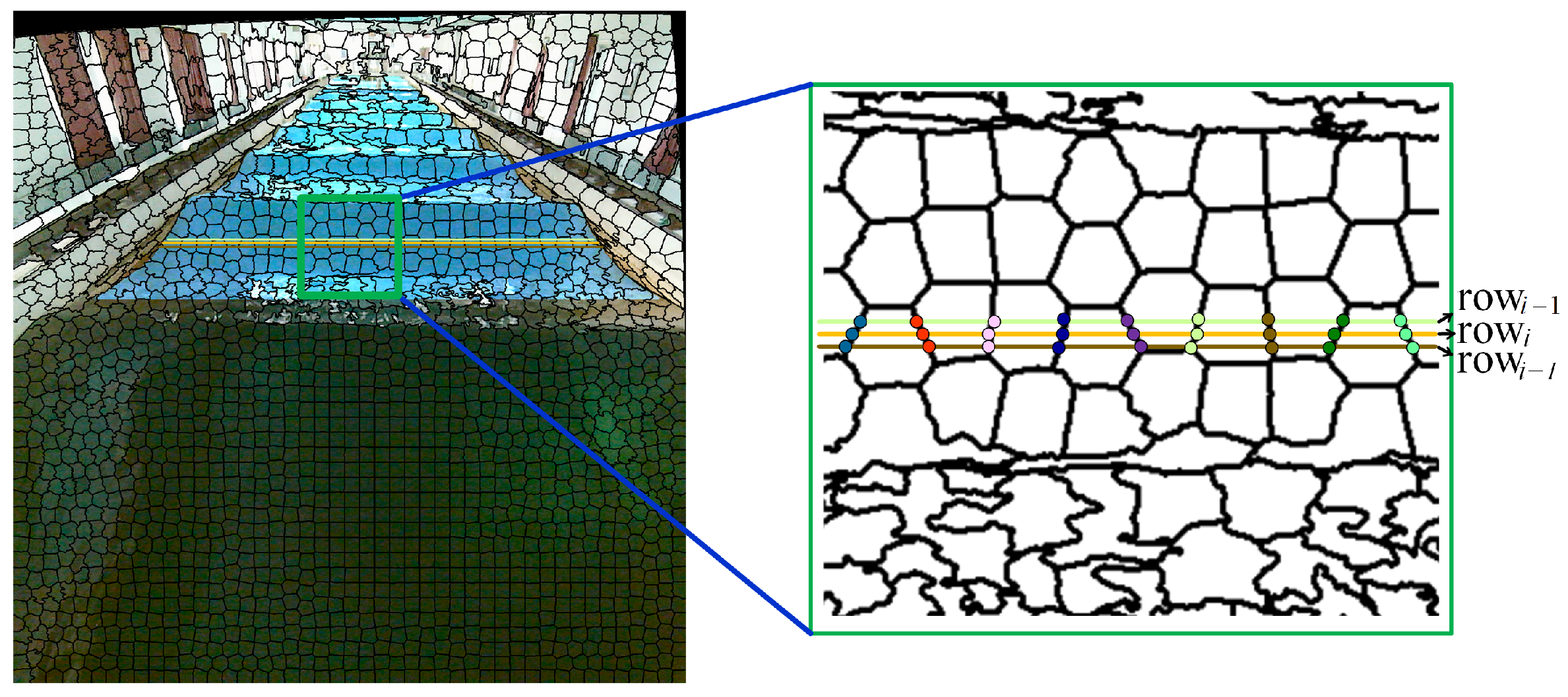
Figure 1. The identification of sparse points by marking the intersections of superpixel boundaries with epipolar lines.
Jmse 13 01699 g001
Figure 2. Matching principle and reconstruction results. (a) The epipolar line segments on the imaging plane are considered as projections of the spatial line segment G H . (b) Comparison results of the two matching methods. The first row shows the results obtained using brute force matching, while the second row shows the results obtained using the perturbation fine matching framework proposed in this study.
Jmse 13 01699 g002
Figure 3. The main process of the proposed 3D reconstruction framework.
Jmse 13 01699 g003
Figure 4. (a) Graph cuts networks without neighborhood smoothness constraints. (b) The uniqueness with o and α in graph cuts network.
Jmse 13 01699 g004
Figure 5. Graph cuts networks with neighbourhood smoothness constraints. (a) Basic network structure with decision nodes o 1 and o 2 connected to source s and sink t. (b) Network with alternative decision nodes α 1 and α 2 for perturbation optimization.
Jmse 13 01699 g005
Figure 6. Cuts for the cases of node α .
Jmse 13 01699 g006
Figure 7. Schematic diagram and photographs of the experimental setup. The origin of the world coordinate system is set in the middle of the baseline of the stereo cameras. The method for calculating the time difference between the frame timestamp and the probe timestamp is Δ t = 22.75 T / λ , where T represents the wave period and λ represents the wave length.
Jmse 13 01699 g007
Figure 8. The instantaneous discrete elevation points with three consecutive frames selected for each condition. The mean value of Y w coordinates is calculated within every 0.01 m range along the Z w direction, thereby determining the elevation of the points.
Jmse 13 01699 g008
Figure 9. Visualization of the reconstructed point clouds from the stereo pairs for four sets of conditions.
Jmse 13 01699 g009
Figure 10. A colored map is used to indicate elevation on the XZ-plane. Firstly, linear interpolation of the elevation values is performed on the XZ-plane. Then, the Mean Absolute Deviation (MAD) is calculated using the elevation values. Finally, the dark red curves of MAD are obtained above the colored map.
Jmse 13 01699 g010
Table 1. Cases of cuts in the graph.
CasesTriggerOriginal StateUpdated State
Case1 g ( o ) = 0 , g ( α ) = 0 f o = 1 , f α = 0 f o = 1 , f α = 0
Case2 g ( o ) = 0 , g ( α ) = 1 f o = 1 , f α = 0 f o = 1 , f α = 1
Case3 g ( o ) = 1 , g ( α ) = 0 f o = 1 , f α = 0 f o = 0 , f α = 0
Case4 g ( o ) = 1 , g ( α ) = 1 f o = 1 , f α = 0 f o = 0 , f α = 1
Table 2. Statistical comparison of wave condition No. 1 and No. 2.
No.FramesWavelength (m)Wave Height (m) R 2
Stereo Truth Error Stereo Truth Error Z [ 5 , 12 ] Z [ 5 , 8.5 ]
1 t 0 3.05163.2004.64%0.13260.1511.60%0.38290.6985
t 0 + 0.3 s 3.04703.2004.78%0.16690.1511.27%0.58470.6613
t 0 + 0.5 s 3.34143.2004.42%0.15500.1503.33%0.50450.7226
2 t 0 2.93513.2008.28%0.18970.2005.15%0.07580.1569
t 0 + 0.2 s 2.96973.2007.19%0.18240.2008.08%0.29170.5837
t 0 + 0.4 s 3.08573.2003.57%0.18050.2009.75%0.30900.6201
Table 3. Statistical comparison of wave condition No. 3 and No. 4.
No.FramesWavelength (m)Wave Height (m) R 2
Stereo Truth Error Stereo Truth Error Z [ 5 , 12 ] Z [ 5 , 8.5 ]
3 t 0 3.98154.205.20%0.31210.3004.03%0.66160.7227
t 0 + 0.2 s 4.09024.202.61%0.28150.3006.17%0.64280.8732
t 0 + 0.4 s 4.06394.203.24%0.30950.3003.17%0.17740.9555
4 t 0 4.15284.201.12%0.38470.4003.83%0.74830.8029
t 0 + 0.2 s 4.11544.202.01%0.42530.4006.33%0.67550.6619
t 0 + 0.4 s 4.07584.202.76%0.37600.4006.00%0.44790.7608
Disclaimer/Publisher’s Note: The statements, opinions and data contained in all publications are solely those of the individual author(s) and contributor(s) and not of MDPI and/or the editor(s). MDPI and/or the editor(s) disclaim responsibility for any injury to people or property resulting from any ideas, methods, instructions or products referred to in the content.