Abstract
The harsh environment in Arctic regions presents significant challenges to ship stability, particularly when ice accumulation and hull damage occur simultaneously, potentially increasing the risk of instability. This study addresses this critical issue by proposing a comprehensive stability assessment framework for ships operating in Arctic regions. Utilizing the DTMB-5415 ship model, the evaluation integrates both static and dynamic stability under combined ice accumulation and damage conditions. Firstly, an ice accumulation prediction model was developed to estimate ice accumulation over various durations. Subsequently, the static stability of damaged ships with ice accumulation was evaluated. Computational Fluid Dynamics (CFD) simulations were then conducted to calculate roll damping coefficients and analyze the effects of damage location and ice accumulation on free roll decay behavior. A single-degree-of-freedom (SDOF) roll motion model was constructed, incorporating roll damping coefficients and wave excitation moments to simulate roll responses in random wave environments. Extreme value prediction was employed to estimate the short-term extreme response distribution of roll motions. The results indicate that ship stability decreases significantly when ice accumulation and hull damage occur simultaneously. This integrated framework provides a systematic foundation for evaluating ship stability in the Arctic environment, specifically accounting for the combined effects of ice accretion and hull damage.
1. Introduction
Accelerated global warming has significantly reduced the extent of Arctic sea ice, enhancing the strategic and economic value of high-latitude shipping lanes and natural resources [1]. Despite the considerable advantages of the Arctic route, it presents multiple risks from extreme weather conditions, including complex ice conditions, snowstorms, low temperatures, dense fog and strong winds [2]. In this environment, ship deck ice accumulation and collisions with icebergs and floes represent two common and highly hazardous types of accidents that severely threaten the safety of ship navigation.
To ensure vessel safety in Arctic navigation, Hay [3] investigated capsize accidents caused by ice accumulation. The causes of marine ice accumulation and its safety risks to ships and offshore structures have been systematically examined by numerous researchers [4]. Ice accumulation occurs when spray generated by the interaction between the ship bow and waves is carried onto the deck, where it rapidly freezes in low temperatures. Based on the physical principles of ship ice accumulation, Borisenkovs [5] developed an ice formation rate model based on thermodynamics, though it is not considered the heat exchange effect of seawater spray. Lozowski and Zakrzewski [6] established the first empirical ice accumulation equation through model tests on the US Coast Guard patrol vessel (USCGC Midgett). As research progressed, Dehghani et al. [7] developed a ship ice accumulation prediction model that incorporates spray impact factors, combining heat and mass transfer processes with salinity diffusion, and considering ship motion (heading, speed) and environmental factors (wind speed, direction) to quantify the combined effect of wind-induced and seawater spray on ice formation rate. These studies provide a reliable foundation for predicting ice accumulation on polar vessels.
The harsh Arctic environment significantly impairs ship maneuverability, elevating the risk of collisions with icebergs or other ice bodies, or grounding incidents, which can result in structural damage and compartment flooding, thereby compromising vessel stability and navigational safety. In the field of ship damage stability research, Mancini et al. [8] validated CFD simulations of DTMB 5415 roll decay, confirming their accuracy for large heel angles with proper verification procedures. Begovic et al. [9] further examined intact and damaged conditions, combining CFD and experiments to assess roll damping, though computational demands remain a limitation. Hu et al. [10] employed the Volume of Fluid (VOF) free-surface technique and an overset mesh strategy to solve the Reynolds-Averaged Navier–Stokes (RANS) equations, enabling accurate simulation of ship–wave interactions. Bu et.al. [11] examined a damaged passenger ship at zero forward speed in regular and irregular beam waves through experimental and numerical methods. Xu et al. [12] proposed a Computational Fluid Dynamics (CFD)-based database method for predicting roll responses of damaged ships in beam waves. Bašić et al. [13] employed CFD techniques to predict the total resistance of intact and damaged ship models. Gao et al. [14,15] developed an integrated approach to analyze damaged ship behavior in beam seas by coupling a potential-flow-based seakeeping solver with a Navier–Stokes solver incorporating a VOF model. Gu et al. [16] studied the roll stability of both intact and damaged DTMB-5415 hull forms in beam seas through free-decay and forced roll tests under regular waves. Zhang et al. [17,18] employed a CFD–DEM approach to investigate the influence of ice floe distribution and accumulation on the flooding process and roll motion of damaged ships, whereas in a subsequent study, they integrated experimental and numerical methods to elucidate the critical role of air–fluid interactions in their flooding dynamics and motion responses.
In the analysis of the dynamic stability, roll angle serves as a critical indicator of ship stability. Time-domain simulations are generally regarded as an effective tool for capturing the nonlinear nature of roll motion. Multiple studies have conducted probabilistic evaluations of large-amplitude roll behavior, effectively predicting extreme value distribution of roll angles under various sea conditions and enabling quantification of capsize risk. The Gumbel method and Peak Over Threshold (POT) method are commonly employed extreme value approaches. McTaggart [19] applied the Gumbel extreme value method to ship roll simulations, establishing quantitative relationships between sea-state parameters and capsize probability. Qi et al. [20] analyzed polar ships’ stability under ice conditions using a simplified ice model, CFD-based roll damping, and the ACER method. While extensive research exists on ship icing and damage stability independently, limited attention has been directed toward their combined impact on ship stability.
This study evaluates ship stability under combined ice accretion and damage conditions from both static and dynamic perspectives. Ice accretion calculations over various durations assess its impact on damaged ship static stability. A single-degree-of-freedom roll motion equation is established, and the roll motion extremes under combined wind and wave conditions are predicted using the Gumbel extreme value method. The research systematically investigates the combination of ice accretion and structural damage on dynamic stability, providing an enhanced theoretical foundation and data support for the stability assessment and design of Arctic-operating vessels.
This paper is organized as follows. Section 2 presents the theoretical background of ice accumulation and the calculation of ice accretion over different durations. In Section 3, the static stability of damaged ships under ice accumulation is assessed. Section 4 addresses the dynamic stability evaluation of damaged ships under the combined influences of wind, waves, and ice accretion. In Section 5, the extreme value forecasting of roll motion for damaged ships under icing conditions is discussed. Finally, Section 6 concludes the study.
2. Formulation of Ice Accumulation Models
This section presents a method for calculating ship ice accumulation in Arctic environments, where spray freezing induced by waves, ship motion, and precipitation is considered. Based on mass and energy balance equations, a forecasting model is established and implemented in MATLAB (R2024a) to simulate ice accretion on the DTMB-5415 ship model. Ice mass and the corresponding position of the ship’s center of gravity are calculated for 6, 12, and 18 h under specific environmental conditions.
2.1. Theoretical Background
In the process of ship navigation, sea spray is generated from two sources: the interaction between the ship and the waves denoted as and wind-generated spray denoted as . The distribution of wave-generated spray on the deck is represented by , which represents the mass density of the sea spray at a given height z above the deck. The calculation formula is as follows [21]:
where represents the vertical distance above the deck [m]; denotes the significant wave height [m], as calculated; and is the relative velocity between the ship and the waves [m/s]. The ship speed is defined as the velocity of the ship relative to the Earth’s coordinate system. The calculation formula is expressed as follows:
where represents the wind speed at a height of 10 m, as referenced above the water surface [m/s]; represents the angle between the wind direction and the ship’s course [deg]; represents the ship’s speed [m/s]; and represents the significant wave period [s].
The duration of each spray event, , is calculated as:
The time interval between spray events, , is calculated as:
The frequency of spray events per minute, , is calculated as:
The total duration of spray events per minute, , can be expressed as follows:
The equation governing sea spray motion is expressed as [22]:
where is the spray velocity [m/s], is the air density [kg/m3], is the brine density [kg/m3], and is the drag coefficient, which characterizes the frictional force between droplets and the surrounding air. The calculation formula is expressed as follows:
where is the Reynolds number of the spray.
is defined as another component of sea spray, and represents the mass of water contained in the sea spray per unit volume of the spray cloud. in the vertical direction on the ship deck can be calculated via the empirical formula proposed by Preobrazhenskii [23]. The specific calculation formula is given as follows:
where and are empirical constants defined as follows:
In low-temperature conditions, spray landing on the ship deck undergoes partial rapid solidification into ice, while the remaining portion maintains its liquid state as a saltwater film. The ice accumulation coefficient n provides a quantitative measure for analyzing these distinct portions. Specifically, n represents the fraction of spray that transforms into ice accumulation on the deck, while (1 − n) denotes the portion that remains as a saltwater film. The ice accumulation coefficient n is bounded between 0 and 1. The determination of surface ice accumulation and the ice accumulation coefficient requires consideration of both mass and energy conservation principles.
The mass balance equation enables the calculation of ice accumulation quantity and thickness within a unit grid. The calculation formula is expressed as follows:
where represents the total mass of spray that has frozen into ice [kg/m2.min]; represents the total mass of spray that has formed the saltwater film [kg/m2.min]; and represents the total mass of spray that has evaporated [kg/m2.min].
represents the total amount of spray per minute. By combining the previously calculated sea wave spray mass and wind spray amount, the total spray can be computed. The calculation formula is given as follows [24]:
where represents the wave-generated spray per minute, represents the wind-generated spray per minute, represents the shape coefficient, represents the total duration of wave droplets per minute [s], represents the collision efficiency, and is the relative wind speed of the ship [m/s].
The mass of ice can be calculated as follows:
where represents the ice density [kg/m3], and represents the rate of change in the ice thickness with respect to time.
The mass of the saltwater film can be calculated as follows:
where is the density of the saltwater film [kg/m3]; and is the rate of change in the saltwater film thickness with respect to time.
The increase in ice thickness [mm/h] is given by the following:
After the air-cooled seawater droplets reach the surface of the ship structure, they freeze due to four main heat fluxes at the air–water interface: sensible heat flux , latent heat flux of evaporation , released heat , and radiation heat flux . The heat balance equation is based on Dehghanisanij [24] as follows:
where represents the density of ice [kg/m3]; denotes the latent heat of ice melting [J/kg]; indicates the interface distribution coefficient; is the heat transfer coefficient [W/(m2·K)]; represents the seawater–air interface temperature [K]; denotes the air temperature [K]; represents the Boltzmann constant [W/(m2·K4)]; indicates the droplet temperature [K], and represents the linearization constant of the radiative heat flux [K3].
The temperature [°C] of the brine film on the freezing surface is a function of the salinity of the water film and is expressed as follows [24]:
where represents the salinity of the brine film, which is related to the freezing coefficient and the salinity of the seawater, and is expressed as follows [24]:
Through the integration of mass conservation and energy conservation principles, the numerical solution for the ice accumulation coefficient n under specified operating conditions can be calculated. Based on this parameter, the ice thickness increment within the designated time interval for each unit grid is determinable. The ice volume and corresponding mass for each grid unit can be derived by multiplying this thickness value by the respective grid area and ice density.
2.2. Ice Accumulation Prediction
This research utilizes the DTMB-5415 ship model as the study object, with its primary ship parameters presented in Table 1. The target ship undergoes simplification and discretization for analysis based on the geometric characteristics of the ship deck structure.

Table 1.
Main parameters of the DTMB-5415 ship model.
The ship-ice accumulation calculation program is implemented in MATLAB and organized into multiple subroutine modules. These modules cover (i) partitioning the hull surface into computational regions; (ii) computing the spray-droplet flux; (iii) determining the icing coefficient; and (iv) evaluating the center of gravity of the ship with ice accumulation.
The ice accumulation calculations utilize parameters including the ship length, beam, and precise superstructure position as inputs for the calculation program. Due to the geometric complexity of hull complexity, the analysis employs a segmented-simplification approach. Additionally, since ice accumulation occurs primarily on the deck, calculations focus on the deck surface in the bow region. The program requires environmental inputs such as ship speed, wind speed, air temperature, and the relative angle between the ship’s heading and wind direction. The computational workflow is illustrated in Figure 1.
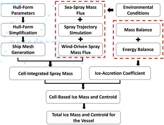
Figure 1.
Computational workflow.
The parameters utilized in the ice accumulation calculation formula are determined based on the research conducted by Dehghani-Sanij et al. [25], as detailed in Table 2.
Table 2.
Calculation parameters of ice accumulation.
Prior to calculating ice accumulation on the surface of ship deck, the deck is discretized into a grid model with cells of 0.25 m2. The droplet distribution, influenced by sea waves and bow structure effects, is determined using Equation (1). By incorporating the droplet trajectory Equation (8), the spatial distribution of spray ice accumulation across the deck is established, as illustrated in Figure 2. The total ice accumulation for the entire deck is computed by aggregating the ice formation across all discrete grid cells. Throughout the simulation, environmental parameters remained constant, with an air temperature of −13.8 °C, wind direction of 180°, and seawater salinity of 34‰.
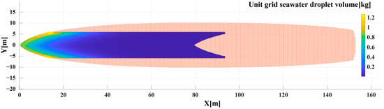
Figure 2.
The distribution of ice accumulation on the deck grid.
The ice accumulation simulation program was executed to model ice formation over periods of 6 h, 12 h, and 18 h. The calculated ice mass accumulation on the hull deck surface and the corresponding center of gravity of the ice-laden vessel for each time interval are presented in Figure 3 and Table 3.
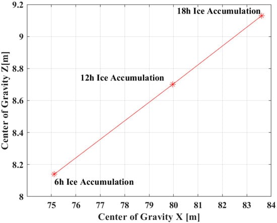
Figure 3.
Center of gravity coordinates of the ship shift.
Table 3.
The resulting ice accumulation.
3. Static Stability of the Ship with Ice Accumulation
This section examines the static stability characteristics of vessels under ice accumulation conditions. The analysis calculates righting arm curves for various damage scenarios and ice accumulation states, providing quantitative evaluation of three key parameters that determine the ship’s floating condition: mean draft [m], heel angle [deg], and trim angle [deg]. The investigation aims to determine how damage and ice accumulation impact vessel floating conditions.
3.1. Research Subject
The DTMB-5415 model features 15 watertight transverse bulkheads that partition the hull into 16 distinct compartments, labeled from NO.1 to NO.16. Figure 4 depicts the arrangement of these watertight bulkheads and compartment divisions.
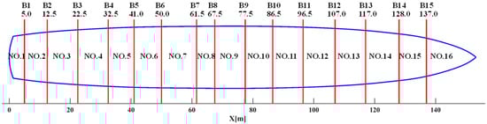
Figure 4.
The division of each compartment.
Referring to the experimental study by Begovic et al. [26] on the DTMB-5415 damaged ship model, this study considers the damage opening shown in Figure 5. The longitudinal extent of the breach opening is less than 15% of the ship length, the top of the compartment remains above the waterline, and the compartment is directly connected to the surrounding sea water, with the internal water level equal to the external free surface. Specifically, three asymmetric flooding scenarios are considered: NO.2–NO.3 (stern), NO.9–NO.10 (midship), and NO.13–NO.14 (bow), with each scenario representing damage to two compartments. The effects on ship stability of these damaged configurations are compared with the intact ship. The positions of the damaged compartments are shown in Figure 4, and the geometric models of the intact and damaged states of DTMB-5415 are shown in Figure 5. The positive Y-direction is established as pointing toward the starboard (right) side of the ship. Bilge keels were not considered in the model.
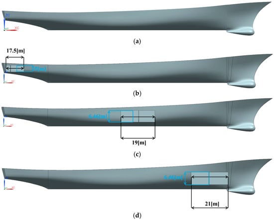
Figure 5.
DTMB5415 geometric model diagram: (a) Intact ship; (b) Damage to the NO.2–NO.3 compartments; (c) Damage to the NO.9–NO.10 compartments; (d) Damage to the NO.13–NO.14 compartments.
3.2. Static Stability Evaluation of the Damaged Ship
This section presents a comparative analysis of floating parameters and static stability between intact and damaged DTMB-5415 ships using real-scale parameters. The damage conditions for the compromised vessel are specified in Section 3.1. The floating state analysis encompasses both the intact condition and multiple damage scenarios. Figure 6 illustrates the restoring arm curve results, while Table 4 provides a comprehensive summary of the floating state variations.
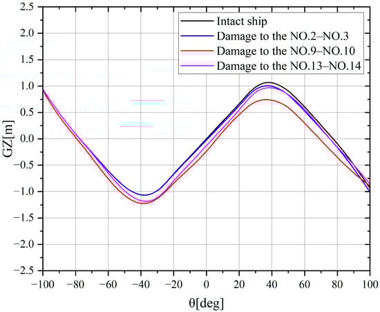
Figure 6.
Comparison of GZ curves of DTMB-5415 intact ship and damaged ship.
Table 4.
Floating conditions of DTMB-5415 in intact and damaged states.
Analysis of Figure 6 and Table 4 reveals that damage to compartments NO.2–NO.3 and NO.13–NO.14 reduces the maximum righting arm by 0.064 m and 0.095 m, respectively, compared to the intact vessel. When compartments NO.9–NO.10 are compromised, the righting-arm curve demonstrates a substantial decrease relative to the undamaged state, with the maximum righting arm diminishing by 0.29 m. The extensive water ingress into the midship compartments significantly shifts the ship’s center of gravity and increases its draft, resulting in an initial heel angle of 7.8 deg. This scenario represents the most severe compromise to the vessel’s stability. Consequently, the midship damage case was selected for subsequent stability assessment following ice accumulation and hull breach.
3.3. Static Stability Assessment of Damage Ships with Ice Accumulation
This section presents a comparative analysis of the floating condition parameters and static stability of the DTMB-5415 full ship model under varying ice accumulation conditions. The analysis examines ice accumulation durations of 6 h and 12 h. Table 3 displays the ice mass and center of gravity coordinates of the iced ship for each duration. The study calculates changes in ship floating conditions across different ice accumulation periods. Figure 7 illustrates the restoring arm curve results, while Table 5 presents the alterations in ship floating conditions.
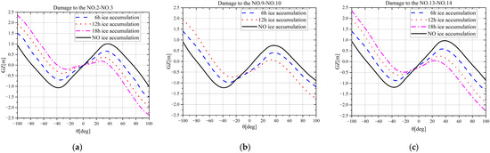
Figure 7.
GZ curves of a damaged ship under varying ice-accumulation durations. (a) Damaged ship in compartments NO.2−NO.3; (b) Damaged ship in compartments NO.9−NO.10; (c) Damaged ship in compartments NO.13−NO.14.
Table 5.
Floating conditions of damaged DTMB-5415 vessels under varying ice accumulation periods.
Figure 7 and Table 5 demonstrate that increasing ice accumulation time under identical compartmental damage conditions leads to significant degradation of the vessel’s static stability. This degradation manifests through reduced righting arm values, in-creased heel and trim angles, and decreased angle of vanishing stability. Among the three damage scenarios analyzed, midship damage (NO.9–NO.10) presents the most severe case: after 12 h of icing, the maximum righting arm decreases by 0.701 m to 0.071 m, falling below the threshold for adequate restoration and necessitating a strict 12 h limit for safe accumulation. Extended exposure to ice accumulation could further compromise the vessel’s stability, particularly if the ice distribution is uneven or if the vessel’s heel recovery capability is impaired. While bow damage (NO.2–NO.3) and stern damage (NO.13–NO.14) maintain relatively higher stability metrics with maximum righting arms of 0.377 m and 0.255 m (representing reductions of 0.621 m and 0.712 m respectively), both conditions still result in significant heel and trim that compromise vessel restoration capacity. The combined impact of hull breach and ice accumulation produces substantial static stability loss, most notably under midship damage conditions.
Evaluating ice accumulation effects on damaged polar vessel stability through righting arm and vanishing stability angle measurements addresses only static stability characteristics, neglecting complex motions in dynamic environments (including waves and wind). This limitation may result in incomplete roll stability assessments. Therefore, implementing a comprehensive dynamic stability loss assessment methodology that analyzes roll motion responses rather than relying exclusively on static stability indicators is essential for ensuring Arctic vessel navigational safety.
4. Dynamic Stability of Damaged Ships with Ice Accumulation Under Combined Wind and Waves
This Section evaluates the dynamic stability of vessels experiencing ice accumulation under wind and wave conditions. A roll motion equation incorporating the combined effects of wind and waves was established, and the resulting response time histories of damaged vessels with ice accumulation were obtained under wind–wave conditions. This approach enables assessment of vessel dynamic stability in extreme sea conditions.
4.1. Model of Ship Roll Motion
Under the combined effect of beam wind and waves, the ship rolling dynamics equation can be simplified into a single-degree-of-freedom form. This equation is then applied to the calculation of the damaged ship, with the specific mathematical expression given as follows [27]:
in the above formula, is the rolling angle; and are the angular velocity and acceleration, respectively; is the relative restoring force coefficient of the ship; and are the linear and squared damping coefficients; represents the relative wave excitation; represents the relative wind excitation; represents the random wave excitation; represents the wind excitation moment; represents the moment of inertia in roll; and represents the added mass moment term.
In the roll motion, wind loads can be classified into two types: steady wind and dynamic wind. Steady wind has a constant wind speed, with its value remaining unchanged over time. However, dynamic wind is characterized by fluctuation of speed and direction that vary with time. In this study, only dynamic wind is considered. To model dynamic wind forces, the classical gust spectrum proposed by Davenport is used, which accurately represents real-world wind fluctuations. The gust spectrum is defined as follows:
in the above formula, is the mean wind speed, , and is the dimensionless variable.
The corresponding steady heeling moment can be analytically calculated using the following formula:
where represents the air density; is the lateral windage area; is the lateral force coefficient; represents the vertical distance from the waterline to the wind pressure center; and represents the vertical distance from the water surface to the wave force center.
In the roll motion, the wave excitation moment is a significant external force that directly affects the ship’s stability in waves. The random wave spectrum corresponding to the wave excitation moment can be expressed using the following mathematical model [28]:
in the formula above: is the wave angular frequency; represents the frequency domain response amplitude of the ship’s rolling moment under unit wave height excitation, which can be numerically solved based on linear potential flow theory; and is the wave energy spectrum density distribution representing irregular sea conditions.
This study implements the wave spectrum model developed by the Joint North Sea Wave Project (JONSWAP). The wave energy spectrum parameterized expression based on the characteristic wave height and period is given as follows:
where is the peak period. Its relationship with other characteristic period parameters (such as the mean zero-crossing period ) shows significant differences compared to the infinite water region. Equation (25) is derived under the assumption of a long-crested waves, which represents a simplification of the sea state conditions considered in this study.
4.2. CFD-Based Calculation of the Roll Damping Coefficient
The precise calculation of the damping coefficient in a rolling motion represents a critical prerequisite for analyzing a ship’s rolling response. The accuracy of this coefficient directly influences the reliability of the predicted motion response. This study establishes a single degree of freedom rolling model, and the rolling damping coefficient is calculated using CFD software StarCCM+ 2406., considering the inflow and outflow of water to the damaged compartments.
This research utilizes the DTMB-5415 ship model with a scale ratio of 1:51 to simulate the free rolling decay motion of the vessel. the model dimensions utilized in DTMB-5415 were kept consistent with those employed in EFD, facilitating the validation process. Previous research on the scale effects between model scale and full-scale vessels has indicated that the influence of free decay experiments conducted to obtain dimensionless natural periods and damping coefficients for roll motion is negligible and can be disregarded [29]. Consequently, the damping coefficient obtained through CFD computations at the model scale with the primary ship parameters presented in Table 1 of Section 2.2 can be employed in subsequent study. The initial conditions specify a speed of 0 knots and an initial heel angle of 28°. The VOF wave is configured to still water. The free rolling decay curve is determined by recording the rolling angle time history in real-time. To manage the large rolling amplitudes during simulation, overlapping mesh technology is implemented, dividing the computational domain into two regions: the background domain and the overlapping domain. The background domain measures 10 m × 3.6 m × 5.4 m, and the boundary conditions are specified as illustrated in Figure 8.
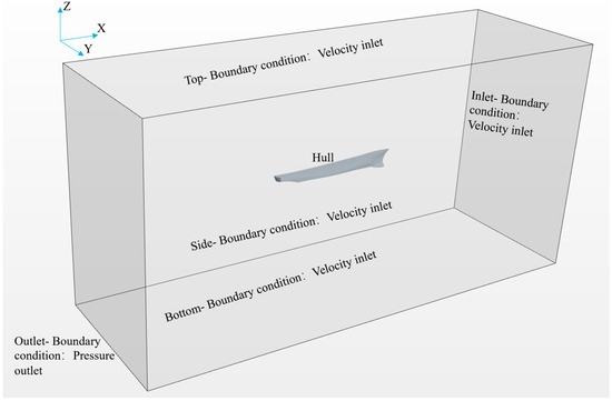
Figure 8.
Computational domain and boundary conditions for the DTMB-5415.
The mesh generation process is performed using the automatic meshing function in STAR-CCM+2406, with a base mesh size of 1 cm and a mesh size for the overlapping domain set to 0.25 cm. The free surface region is refined using anisotropic meshing, with refinement percentages of 50% in the X and Y directions and 2.5% in the Z direction. The hull surface receives 6.25% refinement, while the surface of the computational domain surface is refined to 400%. A cylindrical transition refinement zone between the overlapping and background grids ensures a smooth transition and prevents interpolation errors during rotational motion. The overlapping grid’s prism layer mesh configuration includes 10 prism layers, a 1.3 growth rate, and 25% total prism layer thickness, maintaining a wall Y+ value ≤ 5. The completed mesh comprises 3.41 million cells total, with 1.39 million cells in the background domain and 2.02 million cells in the overlapping domain. Figure 9 illustrates the specific mesh division. The numerical simulations incorporate several models: implicit unsteady solver, cell mass correction, gravity, Eulerian multiphase flow, and the k–epsilon turbulence model. The VOF method simulates the still water wave model. The solver implements second-order time discretization with a 0.005 s time step. The Dynamic Fluid Body Interaction (DFBI) method models the motion in the overlapping region. In the present study, to simulate free-decay motion for the evaluation of roll damping, only the roll degree of freedom was released, while all other degrees of freedom were constrained.
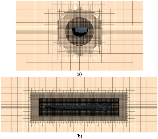
Figure 9.
Mesh division: (a) front view; (b) side view.
The numerical simulation model previously described is utilized to compute the free rolling decay motion. Time step independence and mesh independence verification are conducted, and the free rolling decay curve derived from the simulation is compared with experimental data [8]. To ensure numerical fidelity of the free-decay simulations, both time-step and mesh independence studies are performed. The time-step independence assessment involves repeating the free-decay runs under identical conditions using three different time increments (0.002 s, 0.005 s, and 0.01 s), with the resulting roll-decay histories compared in Figure 10. Subsequently, mesh independence is evaluated following the ITTC grid-refinement guidelines [30] by systematically refining the base mesh according to a grid-refinement ratio. The grid refinement ratio r is defined as follows:
in the formula above, represent the different base grid sizes of the model.
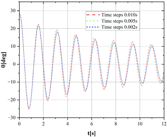
Figure 10.
Comparison of rolling time history curves for different time steps.
Based on a base grid size of 0.01 m, three grid schemes are generated with a refinement ratio of : coarse mesh, medium mesh, and fine mesh. The corresponding base grid sizes are 0.007 m, 0.01 m, and 0.014 m, respectively. Free rolling decay motion simulations are performed for each of these three mesh schemes. The computational results are presented in Figure 11.
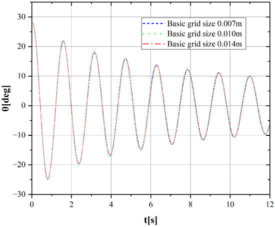
Figure 11.
Comparison of rolling time history curves for different base grid sizes.
The numerical simulations employed various time steps and mesh schemes to evaluate their effects on numerical stability, accuracy, and computational efficiency. Time-step analysis revealed that simulations using 0.002 s and 0.005 s produced consistent roll motion responses with negligible differences, while simulations using 0.01 s demonstrated notable variations in predicted motion. This analysis led to the selection of 0.005 s as the optimal time step, balancing accuracy and computational efficiency. The mesh study incorporated three grid configurations with different base sizes. The numerical results demonstrated minimal sensitivity to grid refinement, confirming mesh independence. The medium mesh scheme with a base grid size of 0.01 m was selected for subsequent analyses, considering computational resources.
Following the time-step and mesh independence analyses, the final simulations utilized a time step of 0.005 s and a base grid size of 0.01 m. The numerical results generated under these parameters were then compared with experimental measurements to assess the accuracy of the methodology, as shown in Figure 12.
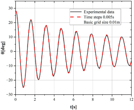
Figure 12.
Comparison of rolling time history curves for experimental data.
Ice accumulation is analyzed as a mass load applied to the vessel to evaluate its parameters under icy conditions. In the simulations, the effects of ice floes and its interaction with the hull were not included. The simulations are conducted for both the intact DTMB-5415 vessel and the damaged vessel with impairment in Compartments NO.13–NO.14, examining three distinct ice accumulation periods. The vessel’s ice mass and center of gravity coordinates under varying ice accumulation durations are detailed in Table 3 of Section 2.2. The computational results are illustrated in Figure 13 and Figure 14.
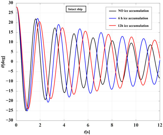
Figure 13.
Comparison of free rolling decay curves for the intact DTMB-5415 ship at different ice accumulation durations.
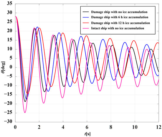
Figure 14.
Comparison of free rolling decay curves for the damaged DTMB-5415 ship at different ice accumulation durations.
As illustrated in Figure 13 and Figure 14, the free rolling decay curves for both intact and damaged ships demonstrate substantial changes with increased ice accumulation duration. Comparative analysis indicates that the damaged ship achieves stability more rapidly than the intact vessel. Furthermore, ice accumulation leads to increased rolling amplitude, while the rolling period exhibits notable changes, characterized by a decelerated decay process. The simultaneous effects of ice accumulation and damage result in an extended rolling period, substantially influencing the ship’s rolling motion. The rolling decay curves are depicted in Figure 15, with the corresponding linear and squared damping coefficients presented in Table 6.
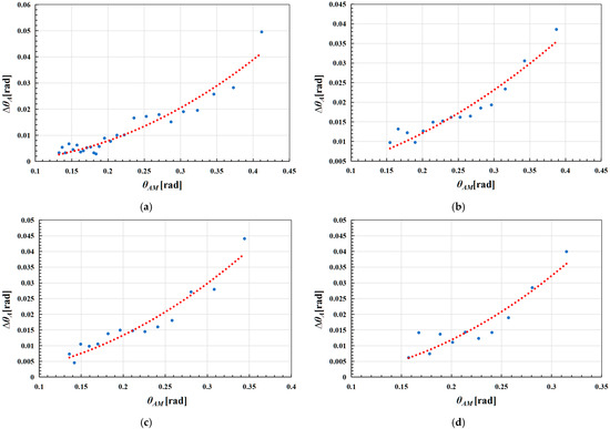
Figure 15.
Rolling decay curves for the intact and damaged ships at different ice accumulation durations: (a) Intact ship after 6 h of ice accumulation; (b) Intact ship after 12 h of ice accumulation; (c) Damage to the NO.9–NO.10 after 6 h of ice accumulation; (d) Damage to the NO.9–NO.10 after 12 h of ice accumulation.
Table 6.
Rolling damping coefficients of intact and damaged vessels under varying ice accumulation periods.
As illustrated in Figure 15 and Table 6, the rolling decay curves of the vessel under ice accumulation demonstrate notable variations. In comparison to the no-ice condition, both linear and squared damping coefficients increase during ice accumulation. The rolling damping coefficients progressively increase with longer ice accumulation duration. Furthermore, the combined effects of ice accumulation and damage lead to additional increases in the rolling damping coefficient, demonstrating that both factors significantly influence the vessel’s rolling damping characteristics.
4.3. Ship Roll Motion Response
CFD methods were employed to conduct numerical simulations of the ship’s free decay roll motion, enabling calculation of roll damping coefficients under various ice accumulation and damage conditions. Based on rolling motion Equation (21), appropriate sea condition parameters were selected, taking into account the vessel’s natural rolling period, wind and wave environmental conditions, and the Beaufort wind scale, as specified in Table 7. Subsequently, roll motion responses were calculated for different sea conditions across four scenarios: intact ship, damaged ship, ship with ice accumulation, and damaged ship with ice accumulation.
Table 7.
Sea condition parameters.
The GZ curves for the intact DTMB-5415, the damaged hull, and both the intact and damaged hulls with ice accumulation are presented in Section 3. Each curve was approximated using a seventh-order polynomial through four primary functions—φ, φ3, φ5, and φ7. Following the previously described methodology, the corresponding righting-moment terms were calculated, and the righting-moment coefficients for the various operating conditions are presented in Table 8.
Table 8.
Righting-moment coefficients.
The wave–energy spectrum was represented by the JONSWAP model, which uses sea-state parameters corresponding to Beaufort scale 7 (significant wave height Hs = 4.0 m; peak period Tp = 11.0 s). Under the assumption of potential-flow theory, the commercial hydrodynamic solver AQWA was employed to calculate the roll moment () experienced by the intact DTMB-5415 when subjected to a unit-amplitude incident wave.
By incorporating the ship roll moment into Equation (24), the wave-excitation moment spectrum associated with the relative excitation moment m(t) was determined. For the specified sea-state parameters, after obtaining the spectrum, a random time series of the excitation was generated through linear superposition. The coefficients of a fourth-order linear filter were identified using the least-squares method, and the single-degree-of-freedom roll motion Equation (21) under combined wind–wave forcing was integrated using a Runge–Kutta scheme to produce the roll–response time history. The roll–motion responses of the intact vessel for the three sea states are illustrated in Figure 16, based on a simulation window of 3600 s.
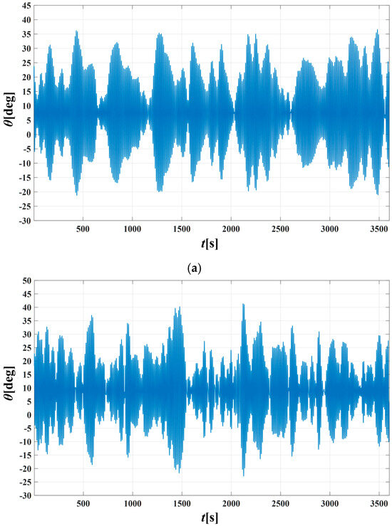
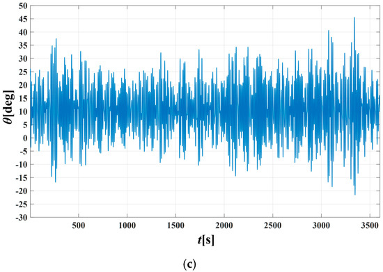
Figure 16.
Roll-motion response of the damaged ship with ice accumulation under combined wind–wave loading: (a) Uw = 15.2 m/s, Hs = 4.0 m, Tp = 10.0 s; (b) Uw = 18.9 m/s, Hs = 5.5 m, Tp = 10.0 s; (c) Uw = 22.1 m/s, Hs = 7.0 m, Tp = 10.0 s.
5. Extreme Value Analysis of the Ship Roll Motion
Ship stability failure frequently correlates with the extreme amplitude distribution characteristics of roll motion. This section employs extreme value forecasting methods to evaluate the stability of ice-damaged ships under combined wind and wave effects. Through prediction of roll angle extreme values, the stability safety margin can be quantified. These analyses provide essential insights for ship design, navigation safety, and emergency management, contributing to safe and stable vessel operations in polar environments.
Extreme value statistics forecasting focuses primarily on analyzing the extreme value probability characteristics of random responses under specific marine environmental conditions, which are typically represented in terms of the probability exceedance form. Let be a random process, and let represent its independent sample sequences. The extreme value statistic is defined as . When the sample sequence satisfies the condition of independent and identically distributed samples with the same cumulative distribution function FX(x), the probability distribution of the extreme value follows the following law:
Regarding the dynamic stability analysis of vessels under wind and wave conditions, ship stability failure occurs when the rolling amplitude exceeds critical thresholds, such as the deck flooding angle or the limit cap angle. Consequently, this study utilizes the absolute response value of rolling motion to construct the random process X(t). Statistical analysis of its extreme value probability characteristics enables the quantification of the vessel’s dynamic stability safety boundaries.
After determining the distribution function through a Gumbel probability plot, the extreme rolling responses corresponding to different exceedance probability levels λ can be calculated.
where is the inverse cumulative distribution function of the Gumbel distribution model.
Following the data-volume recommendations of Chai et al. [31], 50 independent simulations were conducted, each with a duration of 3600 s, to predict roll-motion extremes. From the resulting roll-motion time histories, peak values were extracted, providing 50 samples of maximum roll amplitude. Based on the Gumbel extreme-value model, the sample set underwent linear fitting fitted in an extreme-value probability plot using the least-squares method. Through extrapolation to an exceedance probability of λ = 0.01, the predicted extreme roll angle was determined. Figure 17 illustrates the statistical results for the damaged ship under dead ship conditions with ice accumulation across various sea states. In this case, the icing scenario corresponds to a 12-h accumulation period, and the damage results in asymmetric flooding of compartments NO.13–NO.14, including the fitted Gumbel curves and the forecast extreme value η. In this plot, the horizontal line at λ = 0.01 intersects the fitted curve; the abscissa of this intersection point indicates the predicted extreme roll amplitude.
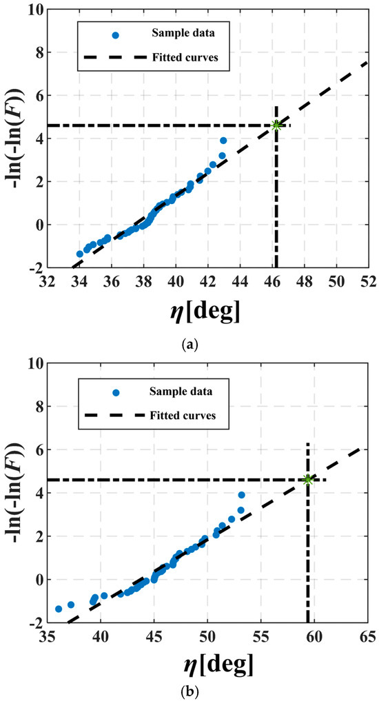
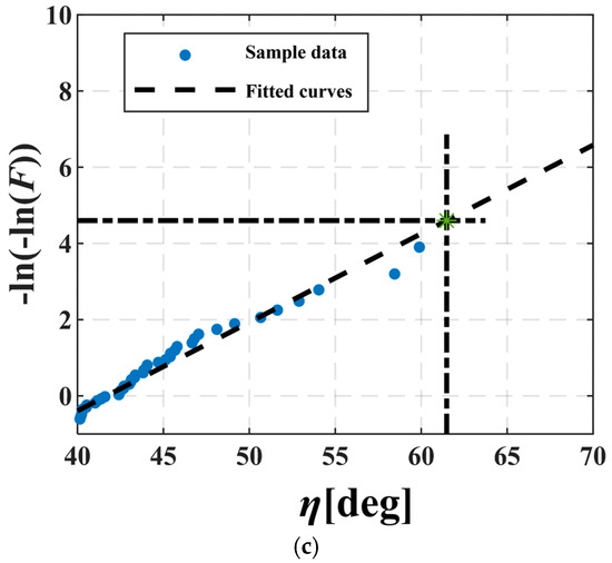
Figure 17.
Extreme-value prediction of roll motion for the damaged ship with ice accumulation under dead-ship conditions subjected to combined wind–wave loading, The green “∗” denotes the roll extreme: (a) Uw = 15.2 m/s, Hs = 4.0 m, Tp = 11.0 s; (b) Uw = 18.9 m/s, Hs = 5.5 m, Tp = 11.0 s; (c) Uw = 22.1 m/s, Hs = 7.0 m, Tp = 11.0 s.
Utilizing the previously described methodology, this paper analyzed the roll extremes of intact and damaged vessels under ice accumulation conditions with varying sea state parameters. The results are presented in Table 9. Figure 17 and Table 9 demonstrate that wave parameters significantly influence the vessel’s roll extremes. The roll angle extremes increase markedly with greater significant wave height, and when the wave characteristic period approximates the vessel’s natural roll period, the roll extremes substantially exceed other cases. In a 9 Beaufort wind environment, the maximum roll extreme of the intact vessel with ice accumulation reaches 49.29°, while the maximum roll extreme of the damaged vessel under identical sea conditions reaches 62.48°. This demonstrates that the roll extremes of the damaged vessel significantly exceed those of the intact vessel. The wave characteristic period notably affects the vessel’s roll extremes, and under identical characteristic periods, both ice accumulation and damage conditions substantially impact the roll extremes.
Table 9.
Roll extremes of intact and damaged vessels under ice accumulation conditions with varying sea state parameters.
6. Conclusions
This study evaluates vessel stability under ice accumulation and damage conditions, examining both static and dynamic aspects. A single-degree-of-freedom roll model was developed, incorporating roll damping coefficients calculated through CFD methods and wave moments computed via potential flow theory. Extreme value forecasting was employed to predict roll response extremes. The study yields several significant conclusions.
- A MATLAB program was developed to calculate ice accumulation over time. Results indicate that ice significantly impacts static stability, particularly in low-temperature, high-wind conditions, resulting in an elevated center of gravity, increased draft, and rapid stability deterioration.
- Vessel damage increases roll angle and reduces stability, particularly in the midship, where the roll angle reaches 7.8° and the maximum righting arm decreases by 0.29 m. Ice accumulation further increases draft and center of gravity, with bow ice inducing a trim angle of 1° to 4° after 6–18 h. The combination of ice accumulation and damage leads to additional stability loss, with both roll and trim angles exceeding 10°, and substantial reductions in static stability parameters.
- CFD simulations reveal that both ice accumulation and damage increase roll damping. After 12 h of ice accumulation, the damping coefficient increases by approximately 8.31%, and with both effects combined, it rises to 0.554. Extreme roll values predicted using the Gumbel method indicate that the roll extreme of the ice-damaged vessel can reach 57.08°, representing a 10.78° increase, resulting in significant dynamic stability deterioration.
In summary, the combined effects of ice accumulation and flooding substantially impair ship stability, with their impact amplifying synergistically. These findings enhance understanding of stability behavior under extreme conditions and provide valuable guidance for hull-form optimization, polar-route planning, and safety assessments.
Author Contributions
Conceptualization, W.C. and J.Q.; methodology, W.C.; software, J.T. and X.Y.; validation, J.Q. and X.Y.; formal analysis, C.W.; investigation, X.Y.; resources, W.Z.; data curation, J.T.; writing—original draft preparation, J.T.; writing—review and editing, W.C., W.Z. and C.W.; visualization, J.T. and X.Y.; supervision, W.C.; project administration, W.C.; funding acquisition, W.C., C.W. and W.Z. All authors have read and agreed to the published version of the manuscript.
Funding
This work is supported by the National Natural Science Foundation of China (52201379) and the project of Wuhan University of Technology Start Up Found for Talented Researchers (WUT-HBQNBR2021-04).
Data Availability Statement
Data will be made available on request.
Conflicts of Interest
The authors declare no conflicts of interest.
References
- Krivorotov, A. The quest for the ultimate resources: Oil, gas, and coal. In Global Arctic: An Introduction to the Multifaceted Dynamics of the Arctic; Springer: Berlin/Heidelberg, Germany, 2022; pp. 257–278. [Google Scholar]
- Lee, S.J.; Jung, K.H.; Ku, N.; Lee, J. A comparison of regression models for the ice loads measured during the ice tank test. Brodogr. Int. J. Nav. Archit. Ocean. Eng. Res. Dev. 2023, 74, 1–15. [Google Scholar] [CrossRef]
- Hay, R. Meteorological aspects of the loss of Lorella and Roderigo. Mar. Obs. 1956, 26, 89–94. [Google Scholar]
- Dehghani-Sanij, A.; Dehghani, S.; Naterer, G.; Muzychka, Y. Sea spray icing phenomena on marine vessels and offshore structures: Review and formulation. Ocean Eng. 2017, 132, 25–39. [Google Scholar] [CrossRef]
- Borisenkov, Y.P.; Pchelko, I. Indicators for Forecasting Ship Icing. 1975. Available online: https://apps.dtic.mil/sti/html/tr/ADA030113/index.html (accessed on 15 January 2025).
- Zakrzewski, W.P.; Lozowski, E.P.; Muggeridge, D. Estimating the extent of the spraying zone on a sea-going ship. Ocean Eng. 1988, 15, 413–429. [Google Scholar] [CrossRef]
- Dehghani, S.; Naterer, G.; Muzychka, Y. Droplet size and velocity distributions of wave-impact sea spray over a marine vessel. Cold Reg. Sci. Technol. 2016, 132, 60–67. [Google Scholar] [CrossRef]
- Mancini, S.; Begovic, E.; Day, A.H.; Incecik, A. Verification and validation of numerical modelling of DTMB 5415 roll decay. Ocean Eng. 2018, 162, 209–223. [Google Scholar] [CrossRef]
- Begovic, E.; Day, A.H.; Incecik, A.; Mancini, S.; Pizzirusso, D. Roll damping assessment of intact and damaged ship by CFD and EFD methods. In Proceedings of the 12th International Conference on the Stability of Ships and Ocean Vehicles, Glasgow, UK, 14–19 June 2015; pp. 14–19. [Google Scholar]
- Hu, L.; Yuan, Z.; Liu, J.; Guo, Y.; Liu, W.; Terziev, M. 3-DOF motion response analysis of damaged ships in quartering waves. Appl. Ocean Res. 2025, 161, 104659. [Google Scholar] [CrossRef]
- Bu, S.; Zhang, P.; Liu, H.; Shi, Y.; Gu, M. Researches on the motion and flooding process of a damaged passenger ship in regular and irregular beam waves. Ocean Eng. 2023, 281, 114927. [Google Scholar] [CrossRef]
- Xu, S.; Gao, Z.; Xue, W. CFD database method for roll response of damaged ship during quasi-steady flooding in beam waves. Appl. Ocean Res. 2022, 126, 103282. [Google Scholar] [CrossRef]
- Bašić, J.; Degiuli, N.; Dejhalla, R. Total resistance prediction of an intact and damaged tanker with flooded tanks in calm water. Ocean Eng. 2017, 130, 83–91. [Google Scholar] [CrossRef]
- Gao, Z.; Gao, Q.; Vassalos, D. Numerical study of damaged ship flooding in beam seas. Ocean Eng. 2013, 61, 77–87. [Google Scholar] [CrossRef]
- Gao, Z.; Shi, Z. Numerical study on damaged ship rolling and capsizing in irregular beam waves during quasi-steady flooding. Ocean Eng. 2023, 289, 116308. [Google Scholar] [CrossRef]
- Gu, Y.; Day, A.; Boulougouris, E.; Dai, S. Experimental investigation on stability of intact and damaged combatant ship in a beam sea. Ships Offshore Struct. 2018, 13, 322–338. [Google Scholar] [CrossRef]
- Zhang, X.; Mancini, S.; Li, P. Numerical investigation into the effects of layer and accumulated ice floes on the hydrodynamics performance of the damaged ship. In Proceedings of the ISOPE International Ocean and Polar Engineering Conference, Shanghai, China, 5–10 June 2022; p. ISOPE–I-22-346. [Google Scholar]
- Zhang, X.; Mancini, S.; Liu, F.; Zhu, R. Experimental and Numerical Investigation into the Effects of Air–Fluid Interaction on the Dynamic Responses of a Damaged Ship. J. Mar. Sci. Eng. 2024, 12, 992. [Google Scholar] [CrossRef]
- McTaggart, K.A. Ship capsize risk in a seaway using fitted distributions to roll maxima. J. Offshore Mech. Arct. Eng. 2000, 122, 141–146. [Google Scholar] [CrossRef]
- Qi, J.; Chai, W.; Sinsabvarodom, C.; Cui, M.; Dou, X.; Zhu, T.; Ji, S. Static and dynamic stability of a polar ship in the arctic region with ice accumulation. Ocean Eng. 2025, 319, 120218. [Google Scholar] [CrossRef]
- Lozowski, E.P.; Szilder, K.; Makkonen, L. Computer simulation of marine ice accretion. Philos. Trans. R. Soc. Lond. Ser. A Math. Phys. Eng. Sci. 2000, 358, 2811–2845. [Google Scholar] [CrossRef]
- Dehghani, S.; Naterer, G.; Muzychka, Y. 3-D trajectory analysis of wave-impact sea spray over a marine vessel. Cold Reg. Sci. Technol. 2018, 146, 72–80. [Google Scholar] [CrossRef]
- Preobrazhenskii, L. Estimate of the content of spray drops in the near-water layer of the atmosphere. Fluid Mech. Sov. Res. 1973, 2, 95–100. [Google Scholar]
- Dehghanisanij, A. Theoretical and Experimental Study of Heat Loss and Ice Accretion of Large Structures on Marine Vessels and Offshore Structures. Ph.D. Thesis, Memorial University of Newfoundland, St. John’s, NL, Canada, 2017. [Google Scholar]
- Dehghani-Sanij, A.; Muzychka, Y.S.; Naterer, G.F. Predicted ice accretion on horizontal surfaces of marine vessels and offshore structures in Arctic regions. In Proceedings of the International Conference on Offshore Mechanics and Arctic Engineering, Busan, Republic of Korea, 19–24 June 2016; p. V008T07A021. [Google Scholar]
- Begovic, E.; Day, A.; Incecik, A. An experimental study of hull girder loads on an intact and damaged naval ship. Ocean Eng. 2017, 133, 47–65. [Google Scholar] [CrossRef]
- Hu, L.-F.; Zhang, K.-Z.; Li, X.-Y.; Chang, R.-X. Capsizing probability of dead ship stability in beam wind and wave for damaged ship. China Ocean Eng. 2019, 33, 245–251. [Google Scholar] [CrossRef]
- Jie, Z.; Zailiang, L.; Yan, L.; Wei, C. Extreme value prediction of the roll motion under random seas. Chin. J. Ship Res. 2025, 20, 196–202. [Google Scholar]
- Yang, J.; Wang, T.; Tang, W.; Fan, J. Roll damping prediction for a three dimensional rectangle floating production storage offloading. J. Shanghai Jiao Tong Univ. 2018, 52, 261–267. [Google Scholar]
- Stern, F.; Wilson, R.V.; Coleman, H.W.; Paterson, E.G. Comprehensive approach to verification and validation of CFD simulations—Part 1: Methodology and procedures. J. Fluids Eng. 2001, 123, 793–802. [Google Scholar] [CrossRef]
- Chai, W.; He, L.; Leira, B.J.; Sinsabvarodom, C.; Feng, P. Short-Term Analysis of Ship Capsizing Probability in Random Seas. In Proceedings of the International Conference on Offshore Mechanics and Arctic Engineering, Hamburg, Germany, 5–10 June 2022; p. V002T02A025. [Google Scholar]
Disclaimer/Publisher’s Note: The statements, opinions and data contained in all publications are solely those of the individual author(s) and contributor(s) and not of MDPI and/or the editor(s). MDPI and/or the editor(s) disclaim responsibility for any injury to people or property resulting from any ideas, methods, instructions or products referred to in the content. |
© 2025 by the authors. Licensee MDPI, Basel, Switzerland. This article is an open access article distributed under the terms and conditions of the Creative Commons Attribution (CC BY) license (https://creativecommons.org/licenses/by/4.0/).