Efficient Hydrodynamic Shape Optimization of a Sea-Turtle-Inspired AUH Using an Optuna-Tuned NSGA-II

Abstract

Disc-shaped Autonomous Underwater Helicopters (AUHs) offer superior maneuverability but suffer from high hydrodynamic drag, which limits their operational endurance. To address this challenge, this study proposes a robust optimization framework for a novel sea-turtle-inspired AUH. A parametric hull, governed by two dimensionless shape factors based on modified Myring equations, was established to facilitate systematic exploration. To reduce the high computational cost of direct CFD evaluations, a high-precision Gaussian Process Regression (GPR) surrogate model was constructed from a small dataset of 24 samples. The core methodological innovation is T-NSGA-II, an algorithm featuring hyperparameters that are systematically optimized by the Optuna framework. In comparative evaluations, the T-NSGA-II-generated Pareto front demonstrated clear superiority over the standard NSGA-II, identifying designs with significantly lower drag for an equivalent vertical force. A key scientific contribution of this research is the identification of a distinct performance gap on the Pareto front. This phenomenon is interpreted not as an algorithmic artifact but as a ‘natural gap’, reflecting a deep physical trade-off, with potential underlying causes including a critical transition in flow physics or a topological shift in the optimal hull geometries. This work not only delivers a suite of optimized, practical AUH designs but also presents a powerful, intelligent optimization methodology that is capable of revealing fundamental physical trade-offs in complex engineering problems.

1. Introduction

Autonomous Underwater Vehicles (AUVs) are pivotal technological platforms for modern marine exploration and exploitation, with widespread applications in scientific research, commercial ventures, and national defense [1]. Significant advantages in terms of cost-effectiveness and operational safety are offered by these vehicles [2]. Historically, AUVs have predominantly employed torpedo-shaped, streamlined hull forms [3]. Although this configuration enhances hydrodynamic performance in rectilinear transit, its requirement for considerable maneuvering space results in limited agility [4,5]. With the increasing complexity of underwater missions, the operational capabilities of conventional AUVs are constrained in confined, congested, or obstacle-laden environments; furthermore, the capacity for stationary hovering and precise attitude control is often lacking [6]. To address these limitations, a novel disk-shaped Autonomous Underwater Helicopter (AUH) has been developed by a team at Zhejiang University. This design facilitates horizontal and vertical motion with a zero turning radius, thereby addressing the maneuverability deficiencies inherent in traditional AUVs [7]. The novel disk-shaped AUH is capable of seabed docking and stationary hovering. It exhibits superior horizontal maneuverability and current-withstanding stability in proximity to complex seabed topographies, thus overcoming the operational limitations encountered by conventional AUVs in such challenging near-seabed environments [8,9]. Despite the AUH’s enhanced maneuverability, its non-streamlined hull form typically induces higher hydrodynamic drag, which adversely impacts endurance [10]. Consequently, hydrodynamic shape optimization of the AUH to minimize drag is essential to enhance its practical utility.

Bionics, an engineering design approach that emulates the structures and functions of natural organisms, offers a significant pathway for advancing underwater vehicle technology [11,12], drawing inspiration from the highly efficient swimming, maneuvering, and stabilization capabilities evolved by marine organisms [13,14]. For instance, the ZRAUV, designed to mimic a catfish, features a triangular head that improves stability compared to conventional hull shapes [15]. This study selects the sea turtle as the biomimetic model for an AUH due to its distinctive dorsoventrally flattened, wide-body morphology and rigid carapace, a selection predicated on leveraging its established maneuvering capabilities, inherent stability advantages (particularly during low-speed and near-seabed operations), and the theoretically greater internal volume afforded by its wide, flat physique [16]. 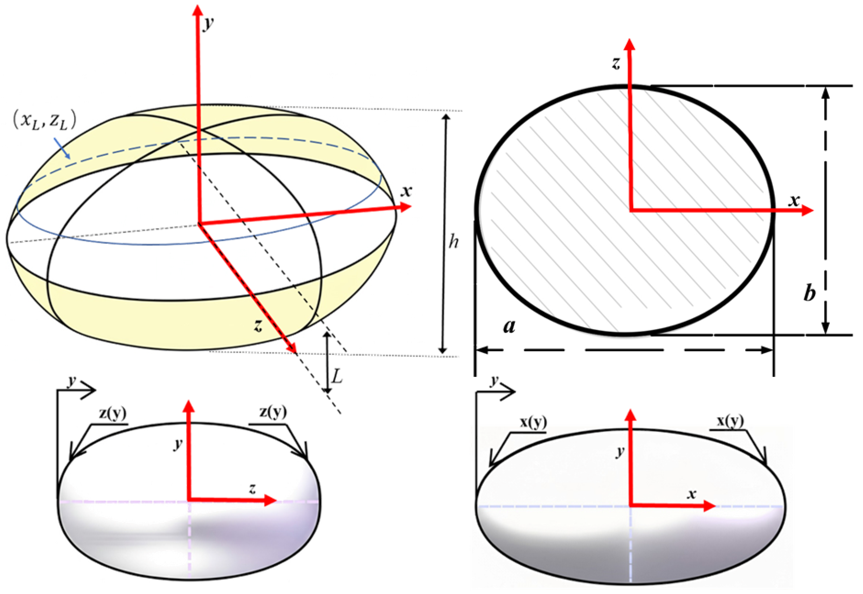However, our approach is not a direct replication of the biological form but rather an integration of key design features with established engineering equations, as conceptually illustrated in Figure 1. Specifically, we drew two primary inspirations from the turtle’s morphology: we adapted its streamlined profile in the lateral view (Figure 1a) and mathematically described it using a modified form of the classic Myring equations; we adopted the wide-body, flattened elliptical planform from its dorsal view (Figure 1b) to enhance stability. By asymmetrically fusing these two core characteristics—one defining the cross-section and the other the planform—we constructed a novel, bio-inspired AUH hull.

Hydrodynamic optimization of the hull form is identified as a crucial pathway for enhancing the performance and reducing the energy consumption of underwater vehicles [17]. At its core, this optimization relies on parametric design methods to systematically explore hull geometries, aiming to minimize drag while adhering to pertinent constraints [18]. For axisymmetric streamlined bodies, Myring introduced classic parametric equations. These equations facilitate the systematic definition and modification of streamlined hull forms through the control of six key parameters: the lengths of the nose, parallel mid-body, and tail sections; the maximum diameter; and various shape indices. This methodology was extensively employed in early Autonomous Underwater Vehicle (AUV) drag reduction optimization efforts [19]. However, when addressing non-axisymmetric or more intricate hull forms, alternative parameterization techniques are often required. For example, B-spline curves were utilized by Ayad et al. to parameterize the bow and stern profiles of a torpedo-shaped AUV. This parameterization, when integrated with genetic algorithms for automated optimization, overcame the flexibility limitations inherent in traditional methods, resulting in an approximate 19% reduction in drag [17]. Similarly, the application of Non-Uniform Rational B-Splines (NURBS) for AUV hull shape parameterization was proposed by An et al. This technique addresses the requirement for a flexible and mathematically robust methodology to define complex, smooth hull surfaces that are amenable to optimization procedures and readily integrable with contemporary CAD/CAM systems [20]. The present study investigates the application of a modified Myring equation for the parameterization of a non-axisymmetric, sea-turtle-inspired AUH hull. This approach is intended to simplify the optimization problem and to assess the adaptability of this established method to novel geometric configurations. The specific modifications implemented and their resultant efficacy are detailed in the subsequent sections of this paper.

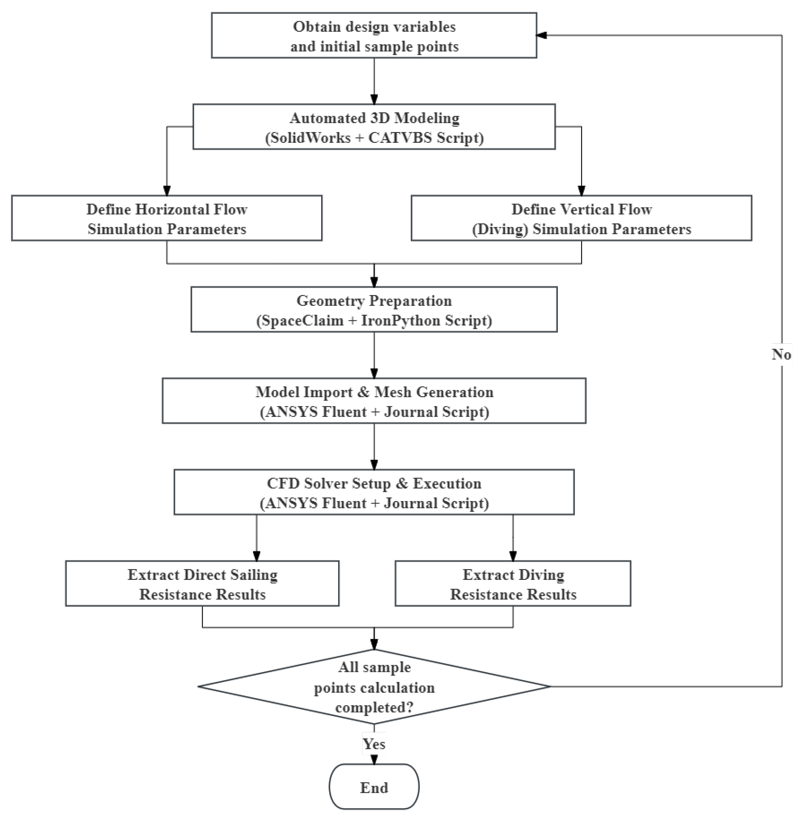
Furthermore, the integration of parametric models with Computational Fluid Dynamics (CFD) for optimization purposes presents substantial computational challenges. Optimization processes typically require the evaluation of numerous candidate designs, and the CFD analysis for each individual design is computationally prohibitive, rendering manual optimization cycles impractical [21]. Consequently, the automation of the CFD-driven optimization workflow is an essential requirement. For instance, Gao et al. addressed AUV hull optimization by developing an automated optimization platform that integrated commercial software packages (iSIGHT, Excel, ICEM, and Fluent), thereby overcoming the inefficiencies associated with manual optimization procedures [19]. Similarly, to address drag reduction for a torpedo-shaped AUV, Ayad et al. established a fully automated optimization platform. This system incorporated B-spline parameterization, CFD simulations, and genetic algorithms, effectively mitigating the time-consuming and labor-intensive nature of manual design iterations [17]. Moreover, Vasudev et al. highlighted the challenges in AUV hull form optimization, where the manual iterative process—which encompasses design parameter modification, geometry and mesh generation, CFD analysis, and drag evaluation—is time-consuming, which hinders the efficient exploration of the vast design space [22]. To overcome these limitations, their approach involved the automated generation of diverse AUV hull forms using parameterized Computer-Aided Geometric Design (CAGD). The SHIPFLOW software was then automatically invoked for geometric modeling, mesh generation, and CFD simulation, with the results subsequently fed back to an optimization algorithm [22]. The present research likewise employs an automated parametric analysis workflow, wherein the parameterized geometric model of the sea-turtle-inspired AUH is closely integrated with CFD simulations.

To further mitigate the substantial computational cost associated with individual simulations within automated CFD optimization workflows, surrogate models are extensively employed in the optimization design of underwater vehicles and other engineering domains [23]. For instance, Song et al. successfully established surrogate relationships between the hull parameters of underwater vehicles and their performance metrics using Kriging models and Latin Hypercube Design (LHD) [24]. Concurrently, at the optimization algorithm level, the Non-dominated Sorting Genetic Algorithm II (NSGA-II) is a frequently used tool, owing to its superior performance in addressing multi-objective optimization problems. This is exemplified by Alam et al., who applied NSGA-II in conjunction with CFD evaluations to acquire the Pareto optimal set for AUV hull forms [22]. However, the performance of evolutionary algorithms such as NSGA-II is known to be highly sensitive to hyperparameter configurations. Inappropriate selection of these parameters can result in diminished optimization efficiency or convergence to suboptimal solutions. Furthermore, within the context of surrogate-assisted optimization for underwater vehicles, the automated and systematic tuning of hyperparameters for algorithms such as NSGA-II has not been extensively investigated. Fortunately, advancements in automated hyperparameter optimization techniques offer promising solutions. The Optuna framework, developed by Akiba et al. is particularly noteworthy, demonstrating significant advantages in enhancing hyperparameter tuning efficiency through its sophisticated sampling and pruning strategies [25]. Therefore, the present study aims to integrate the Optuna hyperparameter optimization framework into the multi-objective optimization of underwater vehicles, specifically when utilizing Gaussian Process Regression (GPR) surrogate models. We leverage Optuna to automatically tune critical NSGA-II hyperparameters. The core objective—under the typical engineering constraints of limited sample sizes and substantial computational costs—is to improve both the optimization efficiency of the NSGA-II algorithm and the quality of the finally obtained Pareto optimal solution set. This approach is intended to provide a more intelligent and efficient solution strategy for such complex engineering optimization problems.

This research proposes an efficient hydrodynamic shape optimization framework for a novel sea-turtle-inspired AUH. Our primary contributions are twofold. First, we propose and parameterize a bio-inspired AUH hull designed to balance hydrodynamic efficiency with the superior maneuverability and stability inherent to the sea turtle morphology. Second, as our core methodological innovation, we introduce an Optuna-tuned NSGA-II (T-NSGA-II) algorithm. This approach systematically optimizes the hyperparameters of the genetic algorithm itself, enhancing its search efficiency and performance when applied to a GPR surrogate model. This method is specifically designed to yield higher-quality Pareto fronts under the constraints of computationally expensive CFD simulations and limited data, offering a more robust and intelligent optimization strategy for complex underwater vehicles.

The remainder of this paper is structured as follows: Section 2 describes the CFD numerical methodology employed and presents the mesh independence study. Section 3 elucidates the automated parametric analysis workflow and the establishment of the GPR surrogate model. Section 4 details the use of Optuna to optimize the NSGA-II hyperparameters. This section further describes the integration of the tuned NSGA-II with the GPR surrogate model for the multi-objective drag reduction optimization of the AUH hull, including the methodology, process, and validation of the results. Finally, an analysis of the optimal solutions obtained by the T-NSGA-II is presented.

2. Numerical Methodology for AUH Simulation

2.1. Geometric Definition of the AUH

An analysis of the morphological characteristics of existing AUHs [20,26,27,28,29] reveals three primary observations: (a) In terms of overall morphology, AUHs predominantly exhibit a distinctive disc-like or saucer-like structure. (b) Owing to this characteristic disc shape, AUHs typically lack the distinct bow and stern sections commonly observed in conventional AUVs. (c) The principal cross-sectional shape of an AUH is generally circular. Although internal configurations may vary, the external wetted surface, which directly interacts with the surrounding fluid, is typically characterized by the continuous, curved surfaces inherent to this disc-like form.

The hull design of the AUH is inspired by the morphological characteristics of sea turtles, aiming to capitalize on the balance they achieve between maneuverability and stability. This biomimetic philosophy results in the AUH being configured as a non-axisymmetric, dorsoventrally flattened, wide-body form. To generate this geometric profile, the classic Myring hull line Equations [30] were adapted and extended, while Myring equations are conventionally employed for designing axisymmetric bodies of revolution; this is a key geometric innovation which, herein, is their extension to define non-axisymmetric hull forms. This allows for more flexible, biomimetically informed control through the incorporation of two independent, dimensionless shape parameters, $n_1$ and $n_2$. The hull surface is defined by the following set of parametric equations:

$$\left\{\begin{array}{c}x=-{\displaystyle \frac{a}{2}}{\left[1-{\left({\displaystyle \frac{2y}{h}}\right)}^{n_1}\right]}^{{\displaystyle \frac{1}{2}}},\hfill \\ z=-{\displaystyle \frac{b}{2}}{\left[1-{\left({\displaystyle \frac{2y}{h}}\right)}^{n_2}\right]}^{{\displaystyle \frac{1}{2}}}\left(y\in \left[0,{\displaystyle \frac{h}{2}}\right]\right),\hfill \\ {\left({\displaystyle \frac{x_L}{x}}\right)}^2+{\left({\displaystyle \frac{z_L}{z}}\right)}^2=1\hfill \end{array}\right.$$

(1)

To provide a detailed description of the parametric model shown in Figure 2, we first define its coordinate system: the x-axis is the longitudinal axis (length), the y-axis is the vertical axis (height), and the z-axis is the transverse axis (width). As governed by Equation (1), the hull’s contour is defined based on the vertical coordinate, y. The first two lines of the equation, representing the core of the modified Myring formulation, calculate the maximum semi-length, x, and semi-width, z, of the hull’s profile at a given height, y. The third line then explicitly defines the local horizontal cross-section at that height as an ellipse, using x and z as its semi-axes, where $x_L$ and $z_L$ are the local coordinates of any point on that elliptical contour.

Within this framework, the two dimensionless shape factors, $n_1$ and $n_2$, serve as the decision variables for our shape optimization. The parameter $n_1$ governs the fullness in the xy-plane (side view), while $n_2$ governs the fullness in the xz-plane (planform view). The global parameters a, b, and h represent the AUH’s overall length, width, and height, respectively. To focus specifically on the influence of the shape factors on hydrodynamic performance, these principal dimensional parameters (a = 600 mm, b = 500 mm, h = 300 mm) are held constant for the present study.

2.2. Optimization Objectives and Decision Variables

The primary objective of the hydrodynamic optimization is to minimize the drag on the AUH hull. Reducing drag is paramount for enhancing the endurance and operational efficiency of AUHs, given their typically limited energy reserves [31]. The optimization process considers two principal operational scenarios: horizontal motion, corresponding to axial flow along the vehicle’s longitudinal (x-axis), and vertical motion, corresponding to transverse flow along its vertical (y-axis). The hydrodynamic drag is quantified by the dimensionless drag coefficient, $C_d$, which is defined in its standard form as follows [32]:

$$C_d={\displaystyle \frac{F_d}{\frac{1}{2}\rho v^{2}A}}$$

(2)

Herein, $F_d$ denotes the total drag force, $\rho$ is the seawater density, v is the free stream velocity, and A is the reference area. Because the definition of the reference area A depends on the direction of motion for non-axisymmetric bodies, the optimization objectives are resolved into two distinct coefficients: the horizontal drag coefficient ($C_{dh}$) and the vertical force coefficient ($C_{dv}$). For vertical motion, the reference area, $A_v$, is the hull’s planform area in the xz-plane; this is a standard ellipse whose area is precisely calculated by the analytical formula $A_v=\pi ·{\displaystyle \frac{a}{2}}·{\displaystyle \frac{b}{2}}$. In contrast, the reference area for horizontal motion, $A_h$, is the maximum frontal cross-sectional area in the yz-plane. As this cross-sectional contour is defined by complex, modified Myring equations and is not a standard ellipse, it lacks a simple analytical formula. To ensure high fidelity, its value was therefore computed numerically for each individual design variant by directly and precisely measuring the area from its 3D CAD model.

The multi-objective optimization undertaken in this study aims to identify a Pareto optimal set of solutions. These solutions represent the optimal trade-offs between minimizing drag during horizontal motion and minimizing drag during vertical motion. Two dimensionless shape factors, denoted as $n_1$ and $n_2$, are introduced as the decision variables for the hull shape optimization. The parameter $n_1$ predominantly governs the longitudinal profile of the hull, thereby influencing its fullness along the major axis of the ellipse. Conversely, the parameter $n_2$ primarily controls the transverse profile, affecting the hull’s fullness along the minor axis of the ellipse. The specific value ranges for these parameters are detailed in

Table 1. Design variables and parameter ranges.

Design Variable	Notation	Minimum	Maximum
Shape factor in the xOy plane	$n_1$	1	4
Shape factor in the yOz plane	$n_2$	1	4

. The objective function for the optimization process is formulated as follows: The decision variables for the hull shape optimization are the two dimensionless shape factors, $n_1$ and $n_2$. The parameter $n_1$ predominantly governs the longitudinal profile of the hull in the xy-plane (side view), while $n_2$ primarily controls the transverse profile in the yz-plane (planform view). The specific value ranges for these parameters, which define the design space for the optimization, are detailed in Table 1. This range was selected to explore a practical design space, avoiding overly sharp (n < 1) or excessively blunt (n > 4) geometries that are hydrodynamically inefficient [30].

The multi-objective optimization undertaken in this study is aimed at identifying a Pareto optimal set of solutions. These solutions represent the optimal trade-offs between the conflicting objectives of minimizing drag during horizontal motion and minimizing drag during vertical motion. This surrogate-assisted multi-objective optimization framework has been proven to be an effective approach for solving complex hydrodynamic shape design problems [21,33]. Therefore, the optimization problem is formally stated as follows:

$$\left\{\begin{array}{cc}\hfill \mathrm{Minimize}:& f_1\left(\mathbf{x}\right)=C_{dh}\left(\mathbf{x}\right)\hfill \\ \hfill \mathrm{Minimize}:& f_2\left(\mathbf{x}\right)=C_{dv}\left(\mathbf{x}\right)\hfill \\ \hfill \mathrm{Subject}\mathrm{to}:& 1\le n_1\le 4\hfill \\ \hfill & 1\le n_2\le 4\hfill \end{array}\right.$$

(3)

where $\mathbf{x}={[n_1,n_2]}^T$ is the vector of decision variables.

2.3. Numerical Methodology for Drag Simulation

The fluid flow surrounding the AUH is governed by the three-dimensional, incompressible Reynolds-averaged Navier–Stokes (RANS) equations. These equations ensure the conservation of mass and momentum within the fluid domain [34]. For an incompressible Newtonian fluid, characterized by constant density and viscosity, the steady-state RANS equations, expressed in Cartesian tensor notation, are presented as follows:

$${\displaystyle \frac{\partial {\overline{u}}_i}{\partial x_i}}=0$$

$$\rho {\overline{u}}_j{\displaystyle \frac{\partial {\overline{u}}_i}{\partial x_j}}=-{\displaystyle \frac{\partial \overline{p}}{\partial x_i}}+{\displaystyle \frac{\partial }{\partial x_j}}\left[\mu \left({\displaystyle \frac{\partial {\overline{u}}_i}{\partial x_j}}+{\displaystyle \frac{\partial {\overline{u}}_j}{\partial x_i}}\right)-\rho \overline{u_i^{\prime }{u}_j^{\prime }}\right]+\rho g_i$$

(4)

In these equations, ${\overline{u}}_i$ represents the time-averaged velocity component, $\rho$ denotes fluid density, t signifies time, $\overline{p}$ is the time-averaged pressure, $\mu$ indicates the fluid dynamic viscosity, and $g_i$ is the body force per unit mass. The term $-\rho \overline{u_i^{\prime }{u}_j^{\prime }}$ is designated as the Reynolds stress tensor; it quantifies the influence of turbulent fluctuations on the mean flow and its determination constitutes the critical closure problem within RANS methodology. The introduction of this tensor renders the system of governing unclosed equations. Consequently, a turbulence model is required to provide closure by modeling this term.

To achieve closure for the RANS equations, Menter’s Shear Stress Transport (SST) k-$\omega$ turbulence model is employed in this study [35,36,37,38]. This model is recognized for effectively integrating the robust and accurate performance of the Wilcox k-$\omega$ model in near-wall regions with the advantageous characteristics of the standard k-$ϵ$ model in free-stream areas, away from solid boundaries. The principal advantages of the SST k-$\omega$ model include its precise near-wall treatment, its enhanced predictive capabilities for flows subjected to adverse pressure gradients, and its superior reliability in forecasting flow separation. These attributes are of critical importance for the accurate prediction of complex flow phenomena and the resultant drag, particularly in the stern region of the AUH.

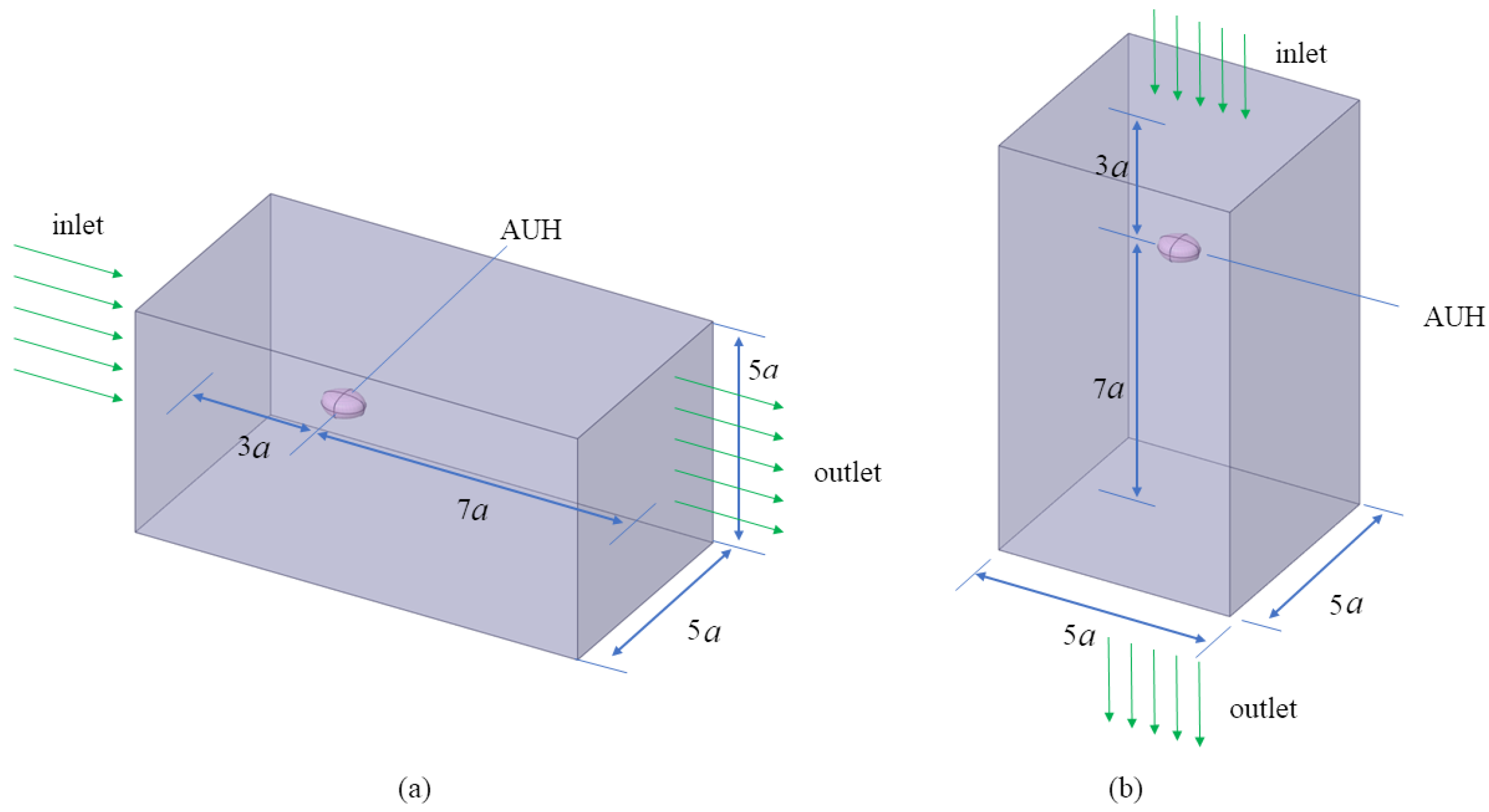
A three-dimensional computational domain is constructed around the AUH hull, as illustrated in Figure 3. To mitigate the influence of boundary conditions, the domain is extended approximately 3a upstream from the bow of the AUH and 7a downstream from its stern, where a represents the characteristic length of the AUH. The transverse width and height of the computational domain are both established at 5a. The boundary conditions are specified as follows: the inlet, located at the upstream boundary of the domain, is defined as a velocity inlet, with a uniform inflow velocity of 1 m/s, approximately 2 knots, which represents a typical low-speed inspection scenario for an AUV, being prescribed. The outlet, positioned at the downstream boundary, is designated as a pressure outlet, where a relative static pressure of zero is specified. The top, bottom, and lateral boundaries of the computational domain are treated as free-slip walls. A no-slip wall condition is applied to the AUH surface, stipulating that the relative velocity of the fluid at this surface is zero.

The computational domain is discretized using an unstructured tetrahedral mesh, a mesh type well-suited to accommodating the complex geometry of the AUH. Mesh refinement is particularly implemented in the vicinity of the AUH hull surface and within the wake region, where high-velocity gradients are anticipated. To accurately resolve the flow details within the boundary layer, multiple layers of prismatic cells, constituting the inflation layer, are generated along the AUH hull surface. This inflation layer is configured with a total of 18 sub-layers; the thickness of the first cell layer adjacent to the hull is 1.8 mm, and a growth rate of 1.2 is applied to the subsequent layers.

To ensure the appropriate application of the SST k-$\omega$ turbulence model, which involves either the utilization of wall functions or the direct resolution of flow within the near-wall region, the dimensionless wall distance, $y^{+}$, of the first grid cell normal to the wall, is verified. The dimensionless wall distance, $y^{+}$, is defined as follows:

$$y^{+}={\displaystyle \frac{y{u}_{\tau }}{\nu }}$$

(5)

Herein, y represents the distance from the center of the first grid cell to the wall, $u_{\tau }$ denotes the wall friction velocity, and $\nu$ is the kinematic viscosity of the fluid. For the prescribed inflow velocity of 1 m/s and a hull length of 0.6 m, the physical properties of seawater are detailed in

Table 2. Physical properties of seawater at 20 °C.

Property	Symbol	Value	Unit
Density	$\rho$	1024	$\mathrm{kg}/{\mathrm{m}}^3$
Dynamic Viscosity	$\mu$	$1.03\times {10}^{-3}$	$\mathrm{Pa}·\mathrm{s}$

. Hydrodynamic simulations are performed utilizing the commercial CFD solver, ANSYS FLUENT(Version 2022 R1). The calculations were conducted using the 3D double-precision solver and executed in parallel mode on a workstation with 10 CPU cores. The working fluid is defined as seawater at a standard temperature of 20 °C. A first-layer thickness of 1.8 mm results in an area-averaged $y^{+}$ value of approximately 40 on the AUH surface. This $y^{+}$ value falls within the range of 30–300, which is appropriate for the wall function approach employed with the SST k-$\omega$ model. To ensure the grid independence of the numerical solutions, a series of simulations with varying mesh densities was conducted [39,40]. Grid convergence is assessed by comparing the drag coefficient values obtained from progressively refined meshes. Convergence is considered to be achieved when the relative difference in the drag values produced by two successively refined mesh densities is less than 2% [41]. For the present study, Case 12 from a predefined sample set was selected as the subject for numerical simulation. Four distinct base mesh sizes were investigated: 20 mm, 12 mm, 10 mm, and 9 mm. The corresponding total number of grid cells for each configuration is presented in

Table 3. Mesh independence study results.

Grid Scheme	Base Grid Size (mm)	Computational Cost (s)	Number of Cells	Horizontal Motion Drag (N)	Relative Error (Straight-Line) (%)	Vertical Motion Drag (N)	Relative Error (Vertical) (%)
Mesh 1	20	502	558,268	12.4067	12.87	76.8279	17.15
Mesh 2	12	1126	1,071,897	11.1358	1.31	68.1015	6.23
Mesh 3	10	3197	1,532,263	11.0113	0.18	66.2552	1.03
Mesh 4	9	3810	2,020,635	10.9919	—	65.5812	—

. Identical inflation layer settings were maintained across all mesh schemes. The results obtained from the finest mesh (Mesh 4) were used as a benchmark to evaluate the relative errors associated with the coarser meshes [33]. Mesh 3, when compared to the finer Mesh 4, exhibits relative errors of 0.18% and 1.03% in the calculated drag for horizontal and vertical motion, respectively. Considering the trade-off between computational cost and solution accuracy, this level of error is deemed acceptable. Consequently, the mesh density configuration of Mesh 3 is selected as the standard for all subsequent hydrodynamic simulations of AUH geometries.

Simulations are performed under steady-state conditions. The Reynolds number (Re), a critical dimensionless parameter characterizing the flow regime, is calculated using the following equation:

$$Re={\displaystyle \frac{\rho VL}{\mu }}$$

(6)

where L denotes the characteristic length. For the present AUH, its overall length, L = 0.6 m, is adopted as the characteristic length. Based on the fluid properties detailed in Table 2, along with the prescribed flow velocity and characteristic length, the Reynolds number is determined to be

$$Re={\displaystyle \frac{1024\mathrm{kg}/{\mathrm{m}}^3\times 1\mathrm{m}/\mathrm{s}\times 0.6\mathrm{m}}{1.03\times {10}^{-3}\mathrm{Pa}·\mathrm{s}}}\approx 5.965\times {10}^5$$

(7)

This Reynolds number indicates a turbulent flow regime. To ensure computational accuracy, the momentum and turbulence transport equations are discretized utilizing a second-order upwind scheme. Pressure–velocity coupling is achieved through the SIMPIEC algorithm. The convergence of the iterative solution process is assessed based on the residuals of the governing equations and the monitored drag force. The computation is considered converged when the normalized residuals for all governing equations fall below ${10}^{-5}$ and the monitored drag coefficient exhibits stability over successive iterations.

3. Surrogate-Model-Based Shape Optimization of an AUH

3.1. Automated Analysis Workflow and Initial Data Generation

In traditional design optimization workflows, the evaluation of each design alternative necessitates several manual steps: modification of the geometric model, regeneration of the mesh, configuration of solver parameters, and execution of simulations. This manual process is time-consuming and susceptible to operational errors that can compromise data consistency [42,43]. Automated workflows can minimize manual intervention through scripted operations. This approach facilitates the automatic modification of AUH model parameters, reconstruction of geometric models, generation of fluid computational domains, discretization of computational grids, and unattended execution of CFD simulations, thereby establishing a seamless data flow from design variable input to performance metric output [44].

The operational instructions and analytical processes governing the entire automated workflow are encapsulated within respective macro files or scripts (VBA, IronPython, Fluent Journal). This encapsulation ensures that, upon invocation, the performance evaluation for an individual design alternative is rapidly and consistently completed solely through the provision of new design variable sample data. Integration among different software modules is realized through standardized file formats and inter-script communication, which guarantees the accuracy of data transfer and the seamless execution of the workflow. The overall workflow for the parametric shape analysis of the AUH is depicted in Figure 4.

3.1.1. Design of Experiments (DOE) for Initial Sample Generation

For the initial Design of Experiments (DOE), 24 sample points were generated using the Optimal Latin Hypercube Sampling (OLHS) method. This method was chosen for three key reasons: its efficiency with computationally expensive simulations, its suitability for small-sample scenarios, and its superior uniformity and space-filling properties. The samples define the two critical design variables for the AUH hull: the shape factors $n_1$ and $n_2$.

The quality of this sampling design is visualized in Figure 5. The marginal probability density functions for each variable (Figure 5a,b), which are estimated from the discrete samples using Kernel Density Estimation (KDE), approximate the ideal uniform distribution. This confirms that the samples exhibit good projection uniformity in each dimension. More importantly, the two-dimensional scatter plot (Figure 5c) illustrates the distribution of the 24 ($n_1$, $n_2$) sample pairs across the entire design space. This scattering visually confirms the method’s space-filling capability. As shown, the points are dispersed evenly, covering the space from the boundaries to the interior without significant clustering or large empty regions. This comprehensive exploration is critical as it ensures a robust and unbiased data foundation for the subsequent construction of the GPR surrogate model [45,46].

3.1.2. Parametric Geometric Modeling of the AUH

Initially, the $n_1$ and $n_2$ values corresponding to a specific sample point are read by the Visual Basic for Applications (VBA) script. Subsequently, the internal parametric model within SolidWorks (Version 2023) is driven by this script, whereby key parameters governing the Myring curve profiles of the AUH bow and stern sections are updated based on these imported $n_1$ and $n_2$ values. Upon completion of the geometric model update, the current three-dimensional model of the AUH is automatically exported by the VBA script as a Standard for the Exchange of Product (STEP) model data file. This procedure ensures that the geometric information is accurately interpreted and processed by the subsequent SpaceClaim software.

3.1.3. Automated Generation of the Fluid Domain

The exported STEP file is automatically imported into SpaceClaim by an IronPython script. Subsequently, this script establishes the fluid computational domain enclosing the AUH, by predefined rules. This process culminates in the generation of a fluid domain geometric model appropriate for CFD analysis.

3.1.4. Automated Computational Fluid Dynamics (CFD) Simulation

A Fluent Journal script file, which incorporates both the fluid domain and the AUH geometry, is invoked to execute the CFD simulations in batch mode. Initially, this script automatically generates the computational mesh. Subsequently, fluid physical properties and boundary conditions are automatically defined; the appropriate turbulence model is selected; and the script configures solver control parameters. For each geometric variant, resistance simulations are automatically performed by Fluent under two distinct operational scenarios: horizontal and vertical motion. The simulations yield the two target objectives: the horizontal drag coefficient ($C_{dh}$) and the vertical force coefficient ($C_{dv}$).

3.1.5. Data Acquisition and Process Iteration

Upon convergence and completion of the CFD simulations for the two operational scenarios corresponding to the current sample point, the requisite performance data—namely, the design variables $n_1$ and $n_2$, along with their corresponding coefficients $C_{dh}$ and $C_{dv}$—are automatically extracted by an external control script from the output files generated by Fluent. These data are then recorded in a structured manner within a predefined Excel spreadsheet. Subsequently, a check is performed by the process to determine whether all 24 OLHS sample points have been processed. Should any sample points remain unprocessed, the procedure reverts to Step 1 (as previously outlined) for the reading and processing of the subsequent sample point. Conversely, once all sample points have been evaluated, the automated workflow is terminated. The resultant dataset, comprising 24 distinct sets of $n_1$, $n_2$, $C_{dh}$, $C_{dv}$ data points, serves as the initial training data for the construction of the GPR surrogate model.

3.2. Construction of the Surrogate Model: Gaussian Process Regression (GPR)

A Gaussian Process defines a probability distribution over a collection of functions. If a function, denoted as $f\left(x\right)$, is assumed to follow a Gaussian Process, then, for any finite set of input points, $x_1,\dots ,x_N$, the corresponding function values, $f\left(x_1\right),\dots ,f\left(x_N\right)$, are characterized by a joint multivariate Gaussian distribution. A Gaussian Process is comprehensively specified by its mean function, $m\left(x\right)$, and its covariance function, $k\left(x,x^{\prime }\right)$, and is formally expressed as follows:

$$f\left(x\right)\sim \mathcal{G}\mathcal{P}\left(m\left(x\right),k\left(x,x^{\prime }\right)\right)$$

(8)

where $x={\left[n_1,n_2\right]}^T$ represents the input vector of design variables utilized in this study. In numerous practical applications, either for model simplification or when prior knowledge is limited, the mean function, $m\left(x\right)$, is commonly assumed to be zero or a simple constant. The covariance function, $k\left(x_i,x_j\right)$, quantifies the correlation between the function values $f\left(x_i\right)$ and $f\left(x_j\right)$ at the respective input points $x_i$ and $x_j$ [47]. In this research, the widely adopted squared exponential kernel function, also referred to as the Radial Basis Function (RBF) kernel or Gaussian kernel, is employed. This kernel function operates under the assumption that the underlying function is infinitely differentiable, implying that it is exceptionally smooth. Its specific mathematical formulation is given by

$$k\left(x_i,x_j\right)={\sigma }_f^{2}exp\left(-{\displaystyle \frac{1}{2l^2}}{∥x_i-x_j∥}^2\right)$$

(9)

In this formulation, the term ${∥x_i-x_j∥}^2$ denotes the squared Euclidean distance between the input points $x_i$ and $x_j$. The hyperparameter ${\sigma }_f^2$, often referred to as the signal variance, governs the extent of variation in the function’s output values; a larger ${\sigma }_f^2$ implies that the function values are permitted to fluctuate over a wider range. The length-scale hyperparameter, l, dictates the “smoothness” of the function within the input space, or, equivalently, the rate at which the correlation between function values at different input points diminishes with increasing separation. A smaller value of l indicates that the function exhibits rapid variations; thus, a strong correlation is observed only between points in close proximity. Conversely, a larger l value signifies a smoother function, where significant correlation may persist even between points that are relatively distant from each other [48]. In practical applications where observations are subject to noise, a target value, $y_i$, is typically modeled as the sum of the true, underlying latent function value, $f\left(x_i\right)$, and an independent and identically distributed Gaussian noise term, ${ϵ}_i$. This relationship is expressed as follows:

$$y_i=f\left(x_i\right)+{ϵ}_i$$

(10)

The noise term, ${ϵ}_i\sim \mathcal{N}\left(0,{\sigma }_n^2\right)$, has a variance ${\sigma }_n^2$ that is also a hyperparameter within the GPR model. It is used to account for uncertainties or noise inherent in the observed data, such as numerical errors originating from CFD simulations. Consequently, for observations that incorporate noise, the diagonal elements of the covariance matrix are augmented by this noise variance term, ${\sigma }_n^2$. This modification is expressed as follows:

$$K_y=K+{\sigma }_n^{2}I$$

(11)

where K is the covariance matrix whose elements are $k\left(x_i,x_j\right)$, and I is the identity matrix. Given a training dataset $\mathcal{D}={\left\{\left(x_i,y_i\right)\right\}}_{i=1}^N$ comprising N observed samples, the objective of GPR is to predict the function output at a new, previously unobserved input point $x_{*}$. The GPR yields a predictive distribution for $p(f_{*}\mid x_{*},\mathcal{D})=\mathcal{N}\left(\overline{f}\left(x_{*}\right),var\left(f\left(x_{*}\right)\right)\right)$. The predictive mean, $\overline{f}\left(x_{*}\right)$, and predictive variance, $var\left(f\left(x_{*}\right)\right)$, of this distribution are given, respectively, by

$$\overline{f}\left(x_{*}\right)=k{\left(x_{*},X\right)}^T{\left(K(X,X)+{\sigma }_n^{2}I\right)}^{-1}y$$

(12)

$$var\left(f\left(x_{*}\right)\right)=k\left(x_{*},x_{*}\right)-k{\left(x_{*},X\right)}^T{\left(K(X,X)+{\sigma }_n^{2}I\right)}^{-1}k\left(X,x_{*}\right)$$

(13)

where X is an N × D matrix containing all training input points, and y is an N × 1 vector containing all training output values. The term $var\left(f\left(x_{*}\right)\right)=k\left(x_{*},x_{*}\right)-k{\left(x_{*},X\right)}^T{\left(K(X,X)+{\sigma }_n^{2}I\right)}^{-1}k\left(X,x_{*}\right)$ denotes an N × 1 column vector where the i-th element is $k\left(x_{*},x_{\mathrm{i}}\right)$, representing the covariances between the test input $x_{*}$ and each training input $x_{\mathrm{i}}$. The matrix $K(X,X)$ is the N × N covariance matrix of the training inputs, with its (i,j)-th element being $k\left(x_i,x_j\right)$. Here, $k\left(x_{*},x_{*}\right)$ represents the prior variance at the test point $x_{*}$ [49], and $k\left(X,x_{*}\right)$ is equivalent to $k\left(x_{*},X\right)$. The predictive mean, $\overline{f}\left(x_{*}\right)$, is utilized as the output of the surrogate model, serving as a computationally inexpensive substitute for costly CFD simulations. The predictive variance, $var\left(f\left(x_{*}\right)\right)$, provides a measure of confidence in these predictions. The set of hyperparameters for the GPR model, $\theta =\left\{{\sigma }_f^2,l,{\sigma }_n^2\right\}$, is not predetermined but is instead learned from the training data by maximizing the marginal log-likelihood function. The marginal log-likelihood function is expressed as follows: $logp\left(y\right|X,\theta )=-{\displaystyle \frac{1}{2}}{y}^T{\left(K_y\right)}^{-1}y-{\displaystyle \frac{1}{2}}log\left|K_y\right|-{\displaystyle \frac{N}{2}}log\left(2\pi \right)$. In this expression, $K_y=K(X,X;\theta )+{\sigma }_n^{2}I$ is the covariance matrix of the noisy observations, given by

$$K_y=K(X,X;\theta )+{\sigma }_n^{2}I$$

(14)

The first term of this function, $-{\displaystyle \frac{1}{2}}{y}^T{\left(K_y\right)}^{-1}y$, represents the data-fit term, which quantifies how well the model explains the training data. The second term, $-{\displaystyle \frac{1}{2}}log\left|K_y\right|$, acts as a model complexity penalty term; this term favors simpler models, thereby aiding in the prevention of overfitting. The final term is a normalization constant. The optimal hyperparameters, $\theta$, that maximize this function are determined through the application of optimization algorithms, such as gradient ascent.

3.3. Surrogate Model Selection and Accuracy Assessment

The selection of a high-fidelity surrogate model is crucial for balancing the high computational cost of CFD simulations with optimization efficiency. In this study, we selected the GPR model, whose predictive capabilities are governed by Equations (15) and (16). To justify the significance of this choice and to demonstrate its superiority, we performed a comparative analysis against two other surrogate models widely used in engineering: the RBF model and the Cubic Response Surface (Cubic RSM) model. To reliably evaluate the generalization performance of these three models, the leave-one-out cross-validation (LOOCV) method is utilized. To quantify and compare their predictive accuracy, standard evaluation metrics, namely the coefficient of determination (R²) and the root mean square error (RMSE), are employed.

$$R^2=1-{\displaystyle \frac{{\displaystyle \sum _{i=1}^N}{(y_i-{\widehat{y}}_i)}^2}{{\displaystyle \sum _{i=1}^N}{(y_i-\overline{y})}^2}}$$

(15)

$$\mathrm{RMSE}=\sqrt{{\displaystyle \frac{1}{N}}{\displaystyle \sum _{i=1}^N}{\left(y_i-{\widehat{y}}_i\right)}^2}$$

(16)

where $y_i$ represents the actual observed value for the i-th sample, ${\widehat{y}}_i$ denotes the value predicted by the model for the i-th sample, $\overline{y}$ is the mean of all actual observed values, and N signifies the total number of sample points. An R² value approaching 1 indicates a superior goodness-of-fit of the model. Conversely, a smaller RMSE value signifies higher predictive accuracy, implying a closer correspondence between the predicted and actual values.

Based on 24 sample points generated via the OLHS method, models—specifically GPR, RBF, and Cubic RSM—are constructed. These models address two distinct optimization objectives: the horizontal drag coefficient ($C_{dh}$) for horizontal motion and the vertical force coefficient ($C_{dv}$) for vertical motion. The fitting accuracy of these constructed models, along with their validation accuracy as determined by LOOCV, is evaluated. The corresponding evaluation results are summarized in

Table 4. Horizontal drag coefficient ($C_{dh}$) fitting accuracy.

Surrogate Method	R2	RMSE
Gaussian Process	0.99999997	0.00000373
RBF (SVR)	0.99132803	0.00214560
Cubic RSM	0.99743148	0.00116770

,

Table 5. Vertical force coefficient ($C_{dv}$) fitting accuracy.

Surrogate Method	R2	RMSE
Gaussian Process	0.99977714	0.00232406
RBF (SVR)	0.85517155	0.05924585
Cubic RSM	0.98590715	0.01848121

,

Table 6. Horizontal drag coefficient ($C_{dh}$) validation accuracy.

Surrogate Method	R2	RMSE
Gaussian Process	0.99970916	0.00038757
RBF (SVR)	0.98453896	0.00282582
Cubic RSM	0.99461292	0.00166802

and

Table 7. Vertical force coefficient ($C_{dv}$) validation accuracy.

Surrogate Method	R2	RMSE
Gaussian Process	0.98182701	0.00648451
RBF (SVR)	0.34055197	0.03906201
Cubic RSM	0.86005734	0.01799448

.

The fitting and validation accuracy data presented in Table 4, Table 5, Table 6 and Table 7 and visualized in Figure 6 provide compelling evidence that justifies the selection of the GPR model. For both optimization objectives ($C_{dh}$ and $C_{dv}$), the R² and RMSE values obtained from GPR are demonstrably and significantly superior to those derived from both the RBF and Cubic RSM models. This direct comparison clearly illustrates that the GPR model effectively learns and reproduces the response characteristics of the training data. Its flexible, non-parametric nature enables the capture of complex non-linear patterns within the data, whereas the RBF and Cubic RSM models, owing to the inherent characteristics of their functional forms, are subject to limitations when fitting intricate responses. For the AUH hull resistance prediction problem, the GPR model, when utilizing just 24 initial sample points, demonstrates comprehensive superiority over these traditional models. The advantages of GPR are particularly pronounced when addressing the resistance during vertical motion, which is characterized by more complex response characteristics.

4. NSGA-II Algorithm with Hyperparameter Optimization Using Optuna

Owing to its efficiency and effectiveness, the NSGA-II is widely adopted as a benchmark algorithm in the domain of Multi-Objective Evolutionary Algorithms (MOEAs) [50]. By incorporating key mechanisms such as fast non-dominated sorting, an elitist preservation strategy, and the calculation of crowding distance, NSGA-II effectively identifies a well-distributed set of Pareto-optimal solutions.

The performance of NSGA-II, however, exhibits significant sensitivity to its hyperparameter settings, including population size and distribution indices for crossover and mutation operators. Suboptimal parameter configurations can lead to issues such as premature convergence to local optima or inadequate diversity maintenance, especially when the algorithm is applied to problems with complex characteristics or when objective function evaluations are computationally expensive.

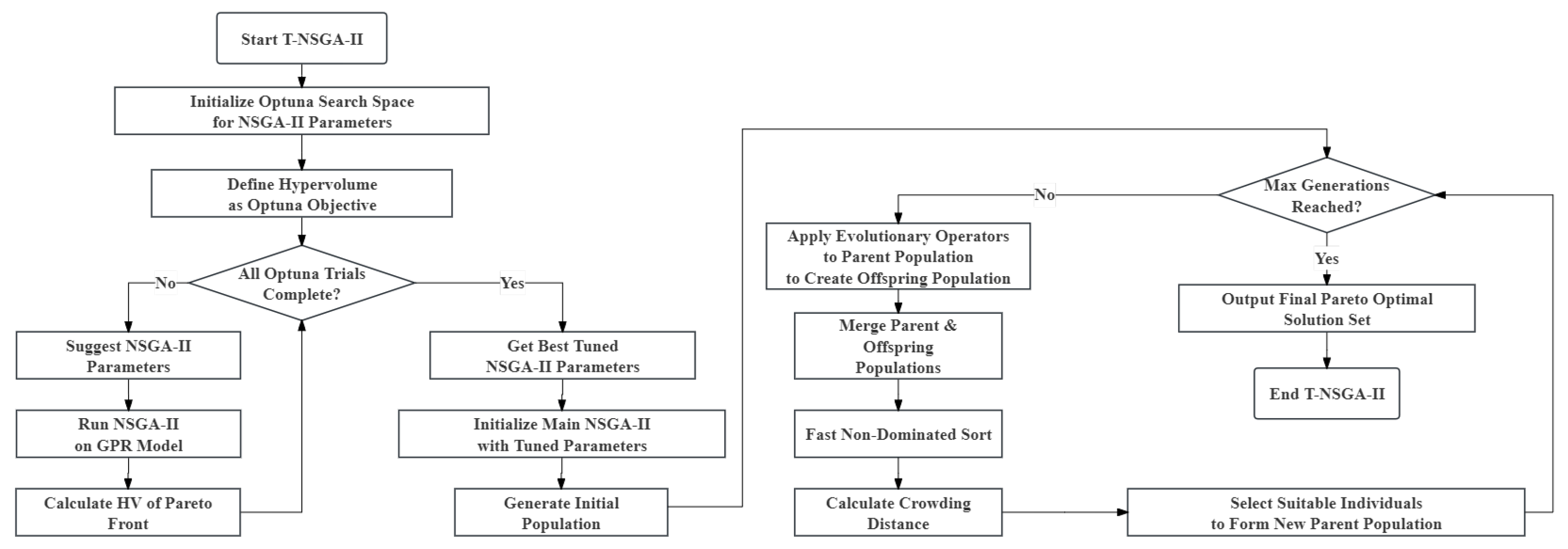
To systematically address this issue of parameter sensitivity and to identify an optimal NSGA-II parameter configuration for the specific AUH external shape optimization task, a hyperparameter optimization strategy leveraging the Optuna framework is adopted in this research. The core of this strategy involves the utilization of Optuna’s advanced search algorithms, wherein the HV indicator is employed as the performance metric. This enables the automatic exploration and determination of the most effective hyperparameter combination for NSGA-II. The NSGA-II algorithm, thus optimized using Optuna, is subsequently referred to as T-NSGA-II in this study.

4.1. The T-NSGA-II Algorithm

The T-NSGA-II method primarily comprises two core stages: (1) the hyperparameter optimization of NSGA-II using Optuna, guided by the HV indicator; (2) the execution of the NSGA-II algorithm with the optimized hyperparameters to address the AUH optimization problem.

The HV indicator is a widely recognized comprehensive performance metric in the field of multi-objective optimization, employed to assess both the convergence and diversity of a set of non-dominated solutions [51]. For a minimization problem involving m objectives, given a set of non-dominated solutions $A=\{s_1,s_2,\dots ,s_{\left|A\right|}\}$ and a reference point $R=(r_1,r_2,\dots ,r_m)$, where the reference point R is dominated by all solutions in A for any $s_i\in A$ and for all objectives j, $s_{i,j}\le r_j$, the HV indicator is defined as the volume of the objective space that is dominated by the solutions in set A and bounded by the reference point R. Its mathematical expression is given by

$$\mathrm{HV}(A,R)=\lambda \left(\bigcup _{s\in A}[s_1,r_1]\times [s_2,r_2]\times \cdots \times [s_m,r_m]\right)$$

(17)

where $\lambda (·)$ denotes the Lebesgue measure in the m-dimensional space. Generally, a larger HV value signifies the superior performance of the solution set in terms of both approximating the true Pareto front and maintaining solution diversity. In the context of this research, the objective of Optuna is to identify a set of NSGA-II hyperparameters that enables the Pareto front, generated by NSGA-II when applied to the AUH problem, to achieve a maximized HV value. This optimization process is efficiently conducted by leveraging evaluations from a pre-trained GPR the surrogate model. The procedure for employing Optuna for hyperparameter tuning to construct the T-NSGA-II algorithm is illustrated in Figure 7. The specific steps involved are outlined as follows:

• The key hyperparameters of NSGA-II are selected for optimization, and their respective search ranges are defined. In this study, the hyperparameters specifically targeted for optimization include population size ($N_{\mathrm{pop}}$), the distribution index for the Simulated Binary Crossover (SBX) operator (${\eta }_c$), and the distribution index for the polynomial mutation operator (${\eta }_m$). The specific ranges for these parameters are detailed in

  Table 8. Hyperparameters and search ranges for T-NSGA-II optimization.

  Name	Symbol	Optuna Tuning Range
  Population Size	$N_{\mathrm{pop}}$	$[40,300]$
  Distribution Index for SBX Crossover	${\eta }_c$	$[5,80]$
  Distribution Index for Polynomial Mutation	${\eta }_m$	$[5,100]$

  .
• An objective function is constructed for the Optuna optimization process. This function encapsulates a single execution of the NSGA-II algorithm: it accepts a set of NSGA-II hyperparameters proposed by Optuna, and subsequently, the NSGA-II algorithm is configured and executed once using these parameters. This execution is performed on the GPR the surrogate model developed for the AUH optimization problem. Upon completion of the NSGA-II run, the HV value of the resulting Pareto front, relative to a predefined reference point, is calculated.
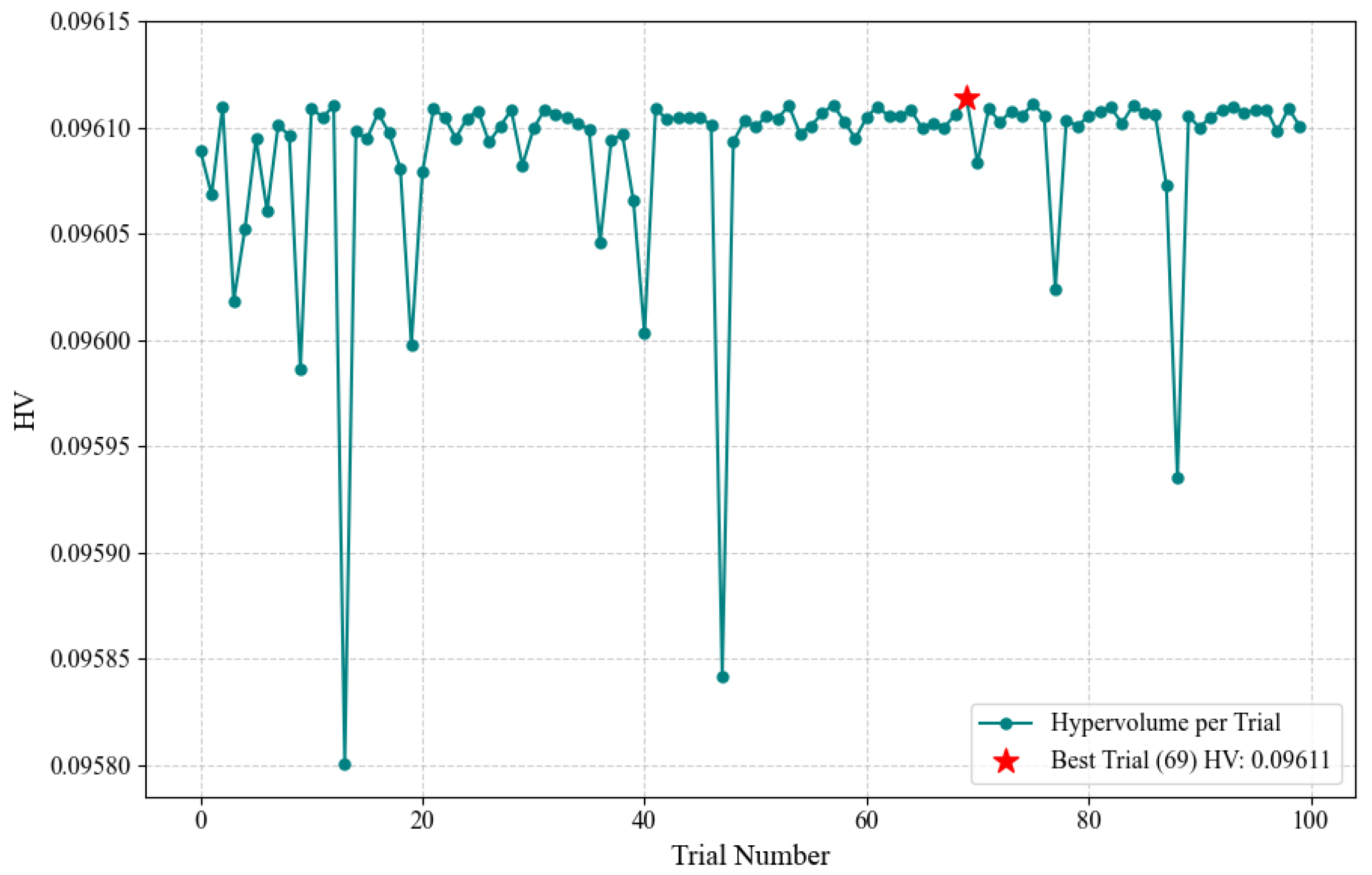
• Optuna is configured to perform a predetermined number of optimization trials. In each trial, a set of hyperparameters is sampled from the defined search space by Optuna’s sampler, and the aforementioned objective function is invoked for evaluation. The Tree-structured Parzen Estimator (TPE), a prominent sequential model-based optimization (SMBO) algorithm, is employed by Optuna. TPE models P (hyperparameters|score) and P(score) iteratively identify hyperparameter configurations that yield favorable performance on the objective function, as depicted by the optimization history in Figure 8.
• Upon the completion of all the trials, the hyperparameter combination yielding the highest HV value across all the evaluations is identified by Optuna. This specific combination is subsequently regarded as the optimal NSGA-II hyperparameter configuration for the current AUH problem. The NSGA-II algorithm, when configured with these optimized parameters, is designated as T-NSGA-II.

4.2. Performance Validation Using Benchmark Test Functions

Benchmark test functions are essential for the evaluation of MOEAs, as they possess known characteristics, including the shape and location of their true Pareto fronts. This enables the convergence and diversity-maintenance capabilities of algorithms to be quantitatively assessed. Consequently, the Zitzler-Deb-Thiele (ZDT) suite of test functions is widely utilized [52]. In the present study, ZDT1, ZDT2, ZDT3, and ZDT4 are selected due to their diverse characteristics: ZDT1 features a convex Pareto front, ZDT2 a non-convex front, ZDT3 a discontinuous front, and ZDT4 exhibits multimodality. The mathematical formulations of these functions are presented in

Table 9. Definitions of the ZDT benchmark test functions.

Test Function	Objective Function and Constraints	Design Variable
ZDT1	$\begin{array}{c}{f}_1\left(x\right)=x_1\\ f_2\left(x\right)=g\left(x\right)\left[1-\sqrt{{\displaystyle \frac{x_1}{g\left(x\right)}}}\right]\\ g\left(x\right)=1+{\displaystyle \frac{9}{n-1}}{\displaystyle \sum _{i=2}^n}{x}_i\end{array}$	$x_i\in [0,1]$ ($i=1,\dots ,n$; ($n=30$)
ZDT2	$\begin{array}{c}{f}_1\left(x\right)=x_1\\ f_2\left(x\right)=g\left(x\right)\left[1-{\left({\displaystyle \frac{x_1}{g\left(x\right)}}\right)}^2\right]\\ g\left(x\right)=1+{\displaystyle \frac{9}{n-1}}{\displaystyle \sum _{i=2}^n}{x}_i\end{array}$	$x_i\in [0,1]$ ($i=1,\dots ,n$; ($n=30$)
ZDT3	$\begin{array}{c}{f}_1\left(x\right)=x_1\\ f_2\left(x\right)=g\left(x\right)[1-\sqrt{{\displaystyle \frac{x_1}{g\left(x\right)}}}-{\displaystyle \frac{x_1}{g\left(x\right)}}sin\left(10\pi x_1\right)]\\ g\left(x\right)=1+{\displaystyle \frac{9}{n-1}}{\displaystyle \sum _{i=2}^n}{x}_i\end{array}$	$x_i\in [0,1]$ ($i=1,\dots ,n$; ($n=30$)
ZDT4	$\begin{array}{c}{f}_1\left(x\right)=x_1\\ f_2\left(x\right)=g\left(x\right)\left[1-\sqrt{{\displaystyle \frac{x_1}{g\left(x\right)}}}\right]\\ g\left(x\right)=1+10(n-1)+{\displaystyle \sum _{i=2}^n}(x_i^2-10cos\left(4\pi x_i\right))\end{array}$	$x_1\in [0,1]$, $x_i\in [-5,5]$ ($i=2,\dots ,n$; ($n=30$)

. For all ZDT functions, the optimization objective involves the minimization of both $f_1\left(x\right)$ and $f_2\left(x\right)$.

To quantitatively compare the performance of NSGA-II and T-NSGA-II, three widely utilized evaluation metrics are employed [53,54,55]. The first of these, Generational Distance (GD), is used to measure the average distance from the set of solutions constituting the algorithm-approximated Pareto front to the true Pareto front. This metric primarily serves to assess the convergence of the algorithm. Its mathematical formulation is given as follows:

$$GD(P{F}_{\mathrm{known}},P{F}_{\mathrm{true}})={\displaystyle \frac{{\left({\displaystyle \sum _{i=1}^{\left|{PF}_{\mathrm{known}}\right|}}{d}_i^q\right)}^{1/q}}{\left|{PF}_{\mathrm{known}}\right|}}$$

(18)

Here, $|P{F}_{\mathrm{known}}|$ denotes the number of solutions in the obtained Pareto front $|P{F}_{\mathrm{known}}|$, and $d_i$ represents the Euclidean distance from the i-th solution in $|P{F}_{\mathrm{known}}|$ to its nearest neighbor in the true Pareto front $P{F}_{\mathrm{true}}$. The parameter q used in the general Minkowski distance, of which Euclidean is a special case is typically set to 2 for Euclidean distance. A lower GD value signifies enhanced convergence of the algorithm. Secondly, the Spacing ($\Delta$) metric is employed to assess the uniformity of the distribution of solutions along $|P{F}_{\mathrm{known}}|$. It is defined as follows:

$$\Delta =\sqrt{{\displaystyle \frac{1}{\left|P{F}_{\mathrm{known}}\right|-1}}\sum _{i=1}^{\left|P{F}_{\mathrm{known}}\right|}{\left(d_i-\overline{d}\right)}^2}$$

(19)

In this context, $d_i$ is defined as follows:

$$d_i=\underset{j\ne i}{min}\left(\sum _{k=1}^m|f_k^i-f_k^j|\right)$$

(20)

where $d_i$ represents the minimum sum of absolute differences in objective function values between a given solution i and any other solution j from $|P{F}_{\mathrm{known}}|$, where $j\ne i$, calculated over all m objectives. The term $\overline{d}$. denotes the arithmetic mean of all such $d_i$ values for the solutions in $|P{F}_{\mathrm{known}}|$. A lower $\Delta$ value indicates a more uniform distribution of solutions along $|P{F}_{\mathrm{known}}|$. A $\Delta$ value of zero signifies that all solutions in $|P{F}_{\mathrm{known}}|$ are perfectly equidistant from their nearest neighbors in the objective space [56]. Thirdly, the Inverted Generational Distance (IGD) metric is employed. IGD assesses both the convergence and diversity of the obtained solution set $|P{F}_{\mathrm{known}}|$ by measuring the average distance from a set of reference points uniformly distributed along the true Pareto front $P{F}_{\mathrm{true}}$ to their nearest neighbors in $|P{F}_{\mathrm{known}}|$. Its mathematical formulation is given by

$$\mathrm{IGD}\left(P{F}_{\mathrm{known}},P{F}_{\mathrm{true}}\right)={\displaystyle \frac{{\left({\displaystyle \sum _{i=1}^{\left|P{F}_{\mathrm{true}}\right|}}{\left(d_i^{\prime }\right)}^q\right)}^{1/q}}{\left|P{F}_{\mathrm{true}}\right|}}$$

(21)

In this formulation, $\left|P{F}_{\mathrm{true}}\right|$ denotes the number of reference points uniformly sampled from the true Pareto front. The term ${d^{\prime }}_i$ represents the Euclidean distance from the i-th reference point in $P{F}_{\mathrm{true}}$ to its nearest neighboring solution within the obtained Pareto front $P{F}_{\mathrm{known}}$. A lower IGD value is indicative of superior overall performance, reflecting both better convergence towards $P{F}_{\mathrm{true}}$ and a more comprehensive representation of it by $P{F}_{\mathrm{known}}$.

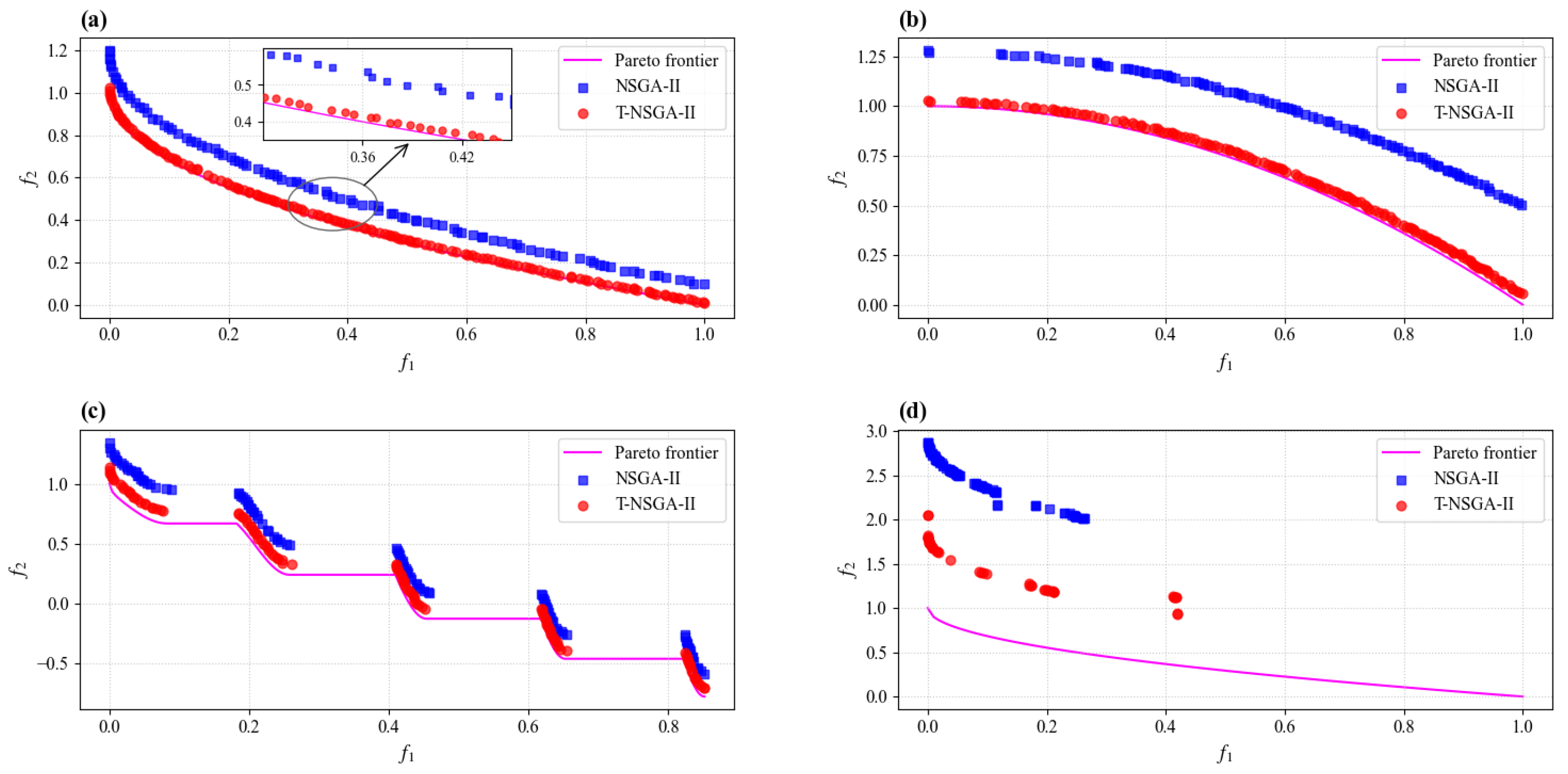
The results presented in

Table 10. Performance comparison of optimization algorithms on ZDT test functions.

Test Function	Evaluation Index	NSGA-II	T-NSGA-II
ZDT1	GD	$8.927\times {10}^{-2}$	$1.210\times {10}^{-2}$
	$\Delta$	$6.266\times {10}^{-3}$	$4.077\times {10}^{-3}$
	IGD	$8.776\times {10}^{-2}$	$1.092\times {10}^{-2}$
ZDT2	GD	$2.509\times {10}^{-1}$	$2.398\times {10}^{-2}$
	$\Delta$	$5.027\times {10}^{-3}$	$3.826\times {10}^{-3}$
	IGD	$2.708\times {10}^{-1}$	$2.358\times {10}^{-2}$
ZDT3	GD	$6.594\times {10}^{-2}$	$2.036\times {10}^{-2}$
	$\Delta$	$8.232\times {10}^{-3}$	$6.501\times {10}^{-3}$
	IGD	$7.949\times {10}^{-2}$	$2.414\times {10}^{-2}$
ZDT4	GD	1.479	$5.339\times {10}^{-1}$
	$\Delta$	$7.169\times {10}^{-3}$	$1.505\times {10}^{-2}$
	IGD	1.716	$6.760\times {10}^{-1}$

and Figure 9 clearly demonstrate the significant advantages of T-NSGA-II when compared to the standard NSGA-II. For the ZDT1, ZDT2, and ZDT3 test functions, T-NSGA-II achieves substantially lower GD and IGD values than those obtained by the standard NSGA-II. This indicates superior performance in terms of both convergence towards the true Pareto front and overall front coverage. Furthermore, the Spacing ($\Delta$) values reveal that the solution distributions generated by T-NSGA-II exhibit either improved or comparable uniformity.

Regarding ZDT4, a function renowned for its numerous local Pareto fronts, T-NSGA-II also exhibits marked improvements in both the GD and IGD metrics. Although the $\Delta$ value for T-NSGA-II on ZDT4 is marginally higher, the substantial gains in convergence, as indicated by GD and IGD, suggest that the optimized hyperparameters enable the algorithm to more effectively navigate the complex search space.

4.3. Application of T-NSGA-II to AUH Shape

Following the validation of its superior performance on benchmark test functions, T-NSGA-II is applied to the primary AUH shape optimization problem. The optimization objectives involve the minimization of both the horizontal drag coefficient ($C_{dh}$) and the vertical force coefficient ($C_{dv}$). For this application, T-NSGA-II utilizes the NSGA-II hyperparameters identified via the Optuna tuning procedure. In contrast, the standard NSGA-II is configured with a default set of hyperparameters for comparative purposes.

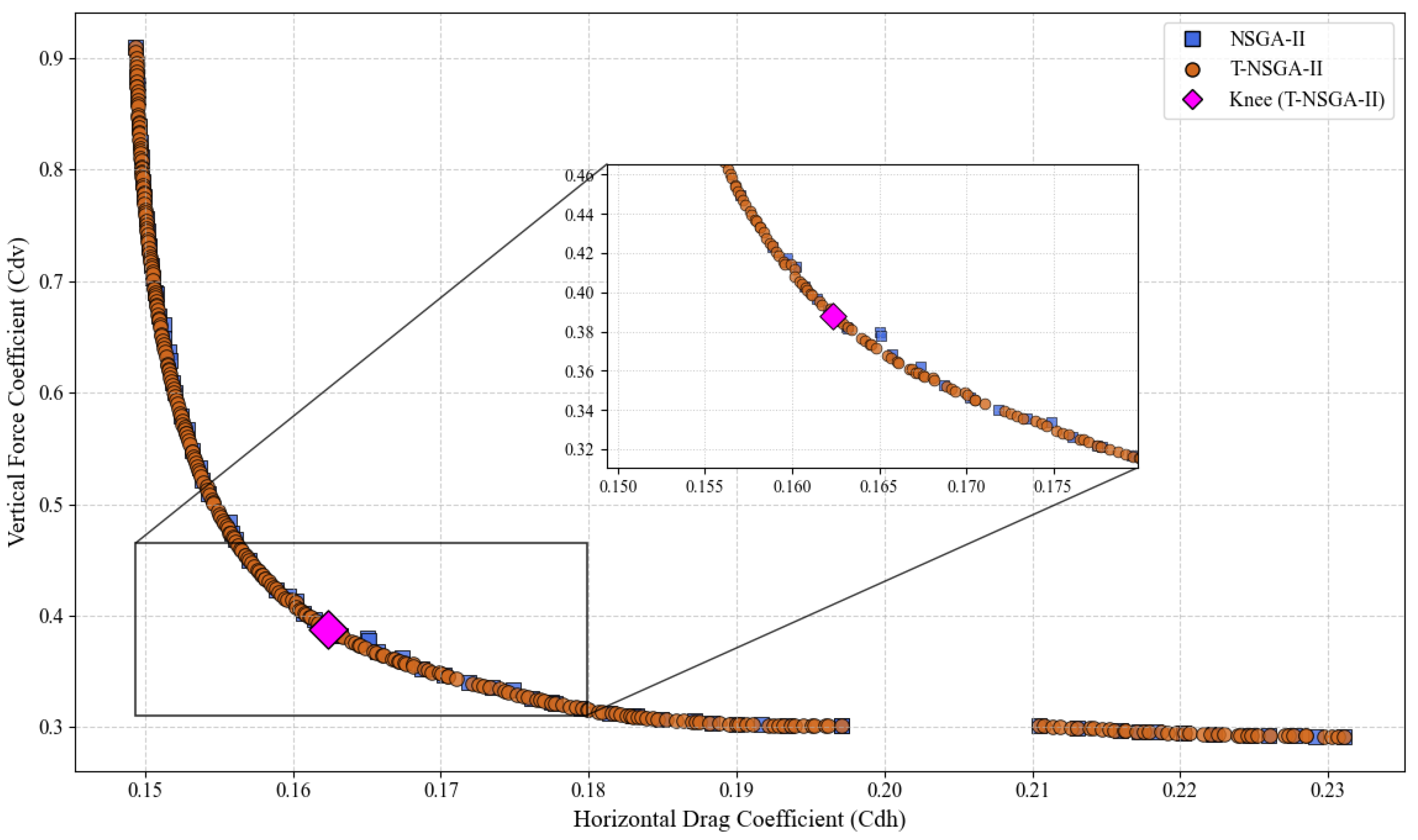
As depicted in Figure 10, the Pareto front generated by T-NSGA-II exhibits clear superiority over that produced by the standard NSGA-II across most regions. For comparable vertical force coefficients, T-NSGA-II consistently identifies solutions with lower drag coefficients. For instance, the representative “knee” point identified by T-NSGA-II, signifying a well-balanced trade-off, dominates all solutions found by the standard NSGA-II in its vicinity. Moreover, T-NSGA-II successfully extends the Pareto front further into the objective space, discovering superior solutions at both extremes of the trade-off spectrum. A notable feature of the T-NSGA-II front is a sparsely populated region, or a gap, observed around $C_{dh}\approx 0.20$. This discontinuity reflects an inherent non-convexity or discontinuity in the problem’s true Pareto front, suggesting that few feasible hull shapes can achieve this specific combination of performance metrics.

The enhanced performance of T-NSGA-II on the AUH optimization problem further substantiates the benefits derived from systematic hyperparameter optimization. With its algorithmic configuration fine-tuned through a learning process involving a GPR surrogate model and Optuna, T-NSGA-II is capable of more effective exploration and exploitation of the search space. Consequently, a set of higher-quality, more dominant Pareto-optimal shape solutions is provided for the AUH design.

4.4. Physical Interpretation of the Pareto Front Discontinuity

A notable finding of this study is a distinct gap, or discontinuity, in the Pareto front generated by the T-NSGA-II algorithm, observed within $C_{dh}$ interval of approximately [0.20, 0.21] in Figure 10. This phenomenon is not considered an artifact of algorithmic failure or insufficient convergence. Instead, its clear identification was enabled by the superior exploratory capability of the tuned T-NSGA-II algorithm. We posit that this is a ‘natural gap’, reflecting a deep physical trade-off inherent in the AUH’s hydrodynamic design space. The underlying physical meaning can be attributed to one or a combination of the following reasons.

First, evidence from our initial dataset supports this conclusion. Analysis of the 24 high-fidelity CFD samples reveals that the design configurations which yield $C_{dh}$ values within this [0.20, 0.21] range are consistently dominated in terms of their $C_{dv}$ by solutions lying outside this range. This indicates that the GPR surrogate model learned from true physical data that this region of the objective space is inherently suboptimal. The optimization algorithm, therefore, correctly identified that no non-dominated solutions exist here.

Second, the gap likely signifies a critical transition in the underlying flow physics. As the hull shape parameters ($n_1$, $n_2$) are varied to push the design into this specific performance interval, the vehicle may be forced into an unstable fluid dynamic regime. This could manifest as an abrupt, large-scale flow separation over the hull’s dorsal surface, a fundamental change in the stern vortex shedding pattern, or a dramatic alteration of the pressure distribution. Such a critical transition would lead to a sudden and significant degradation in performance, making any design within this transitional zone inherently inefficient and thus absent from the Pareto-optimal front.

Third, the discontinuity may represent a topological shift in the optimal hull geometries. The Pareto-optimal solutions on either side of the gap may belong to two distinct families of shapes. For instance, solutions with $C_{dh}<0.20$ might correspond to a family of more slender, streamlined bodies, while solutions with $C_{dh}>0.21$ might belong to a family of blunter, wider bodies optimized for a different hydrodynamic purpose. A smooth, gradual transition between these two distinct optimal topologies may not be possible. To move from one optimal shape family to the other may require a non-trivial, discrete “jump” in the design space, leaving an intermediate performance region that contains no feasible, non-dominated solutions.

In summary, the discovery and clear delineation of this performance gap is a key scientific contribution of this work. It provides invaluable insight for engineers, highlighting a “design trap” or a forbidden performance region that should be avoided in the practical design of such turtle-inspired AUHs. This finding underscores the power of using a robust, well-tuned optimization framework not merely for finding optimal points, but for revealing the deeper, underlying structure of complex engineering design problems.

4.5. Analysis and Interpretation of Multi-Objective Optimization Results

To assess the efficacy of the multi-objective optimization, a detailed comparative analysis of the hydrodynamic performance is undertaken between a baseline initial design, which is the ‘Case 12’ (with parameters $n_1$ = 3.35 and $n_2$ = 1.26) and a selected Pareto-optimal solution (hereinafter termed the ‘optimized design’). The analysis encompasses two critical operating conditions: horizontal and vertical motion. Qualitative comparisons are facilitated through visual inspection of velocity and pressure field contours on the longitudinal plane, while quantitative validation is performed by examining the drag coefficients. 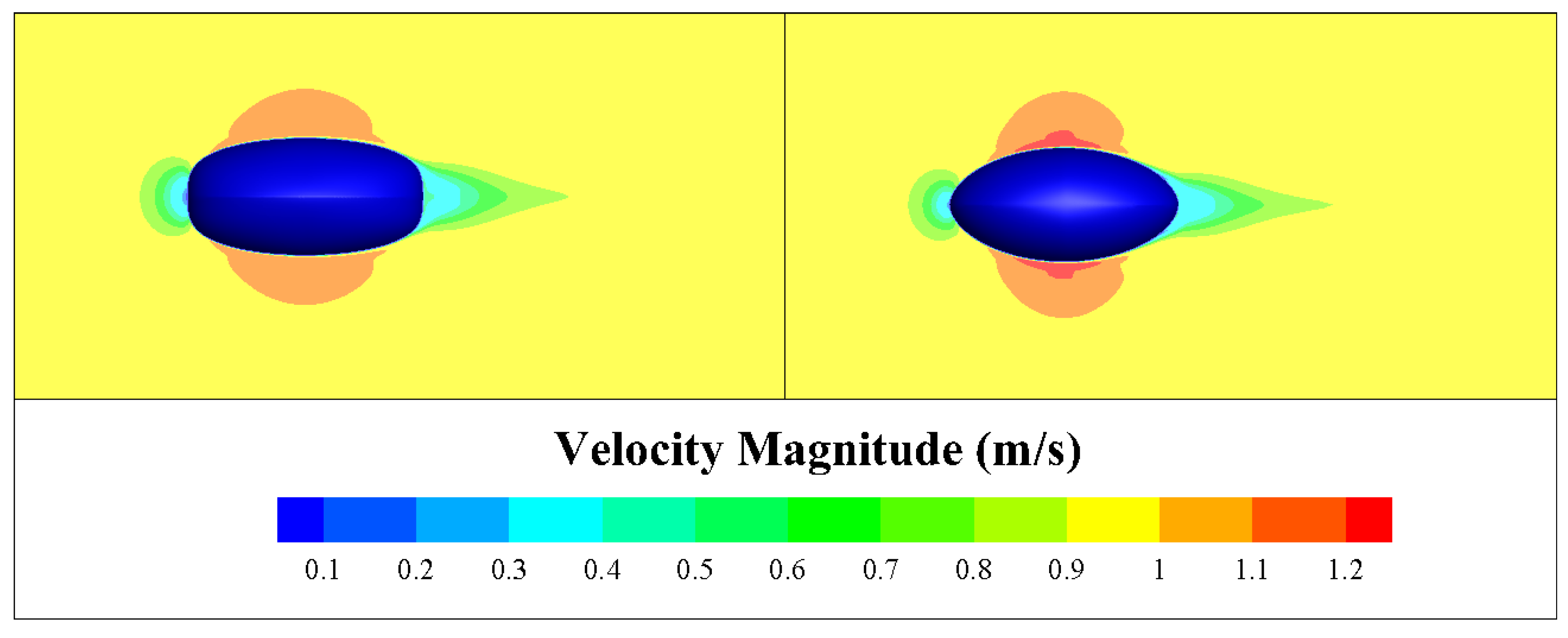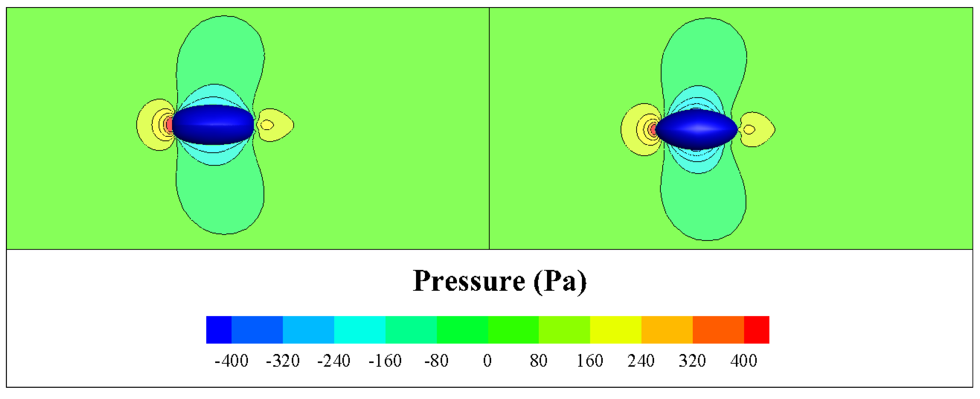Specifically, Figure 11 and Figure 12 present the longitudinal velocity and pressure contours for the horizontal condition, respectively. 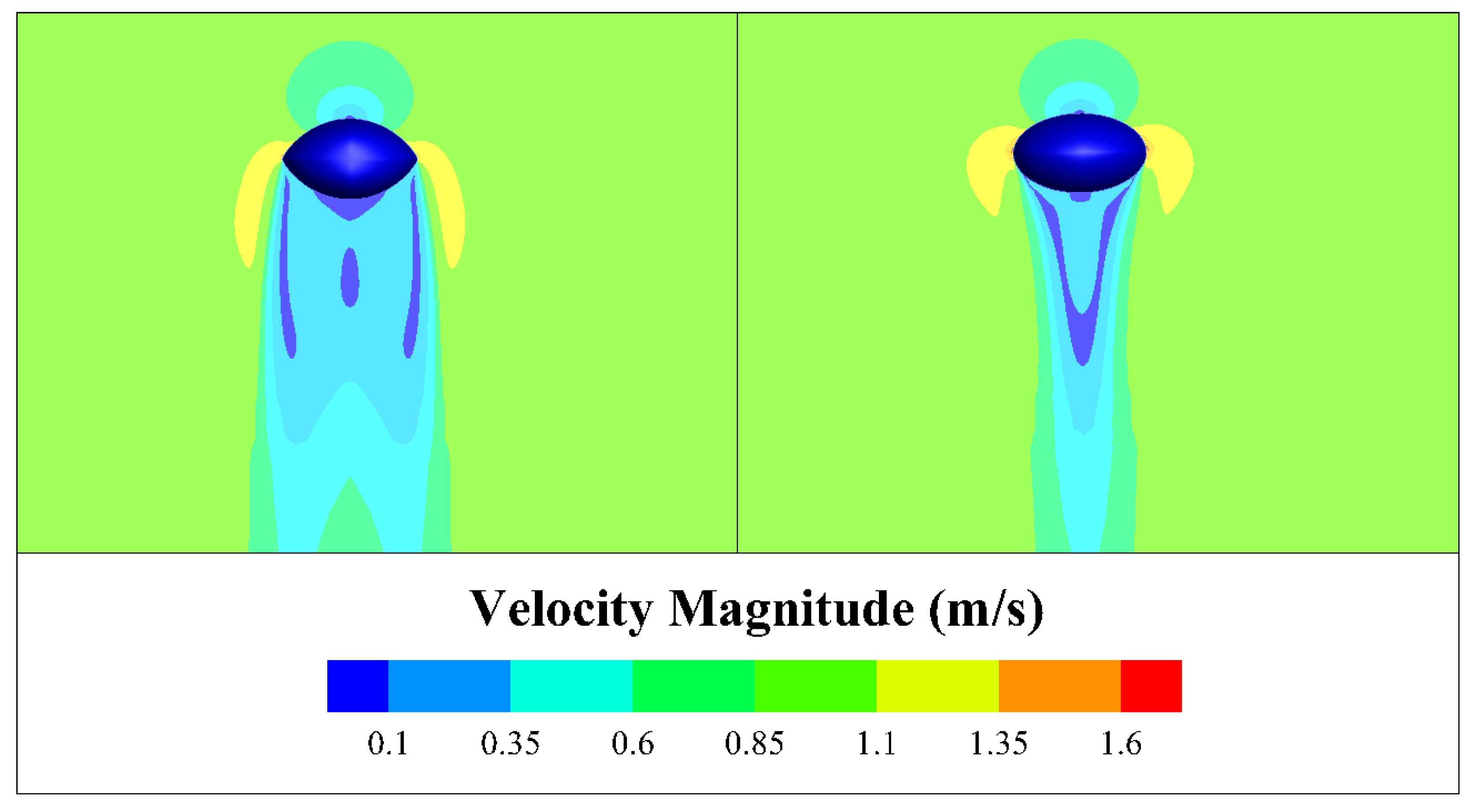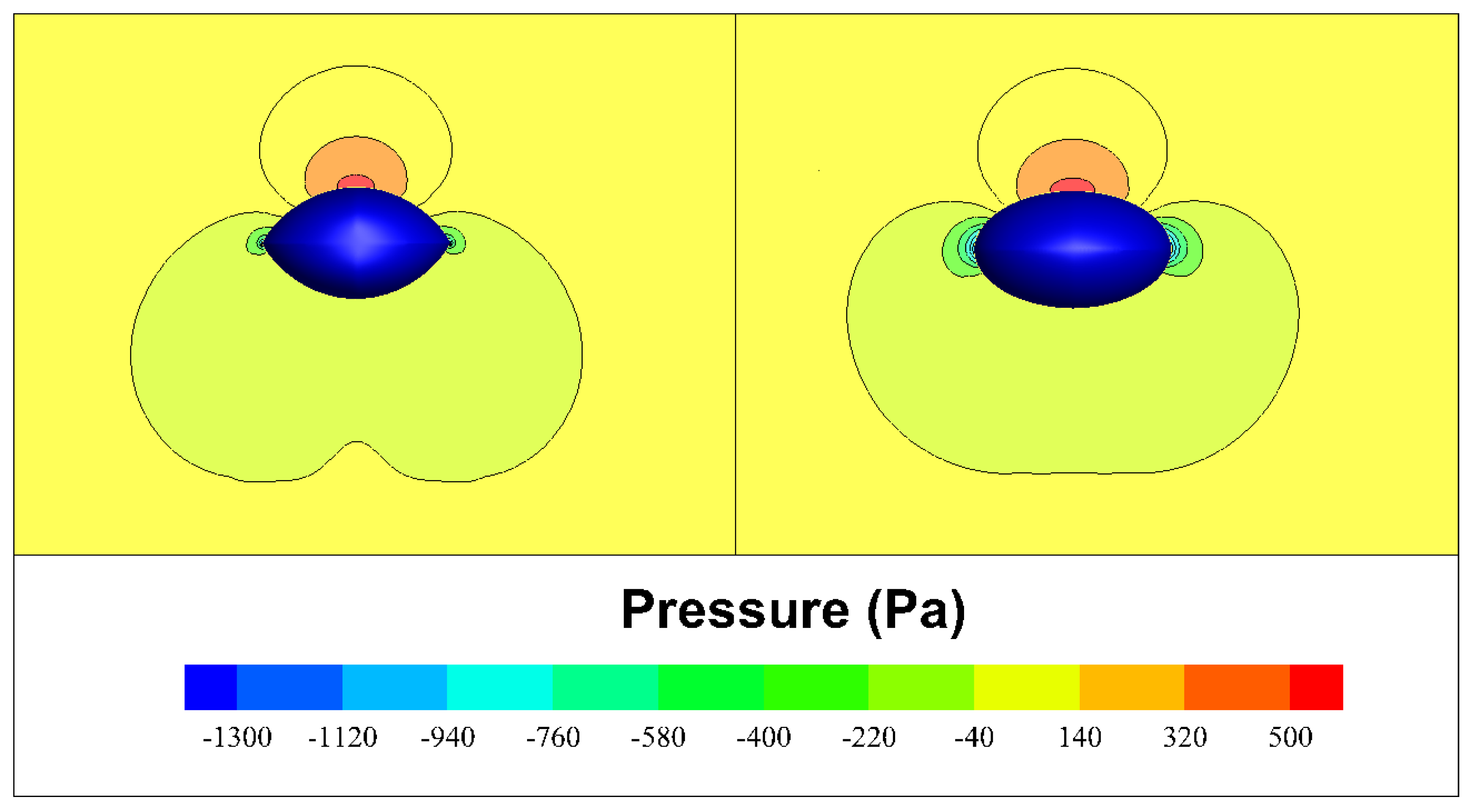Figure 13 and Figure 14 then illustrate the corresponding contours for the vertical condition.

The velocity contours for the horizontal motion condition are presented in Figure 11. For both designs, a wake region characterized by a velocity deficit forms aft of the hull. The initial design generates a broader wake with a more rapidly diffusing low-velocity core. In contrast, the optimized design produces a discernibly narrower and more stable wake, exhibiting a slender morphology and a steeper velocity gradient. This indicates an improved wake quality with reduced disturbance to the surrounding flow field. Figure 12 illustrates the corresponding pressure distributions. The initial design features a more extensive high-pressure zone at the bow and relatively diffuse negative pressure zones along the mid-body. Compared to the initial design, the optimized version significantly attenuates both the extent and peak magnitude of this bow high-pressure zone. Concurrently, its negative pressure zones are more concentrated, resulting in a more compact overall pressure signature. These findings strongly suggest a marked reduction in pressure drag for the optimized design.

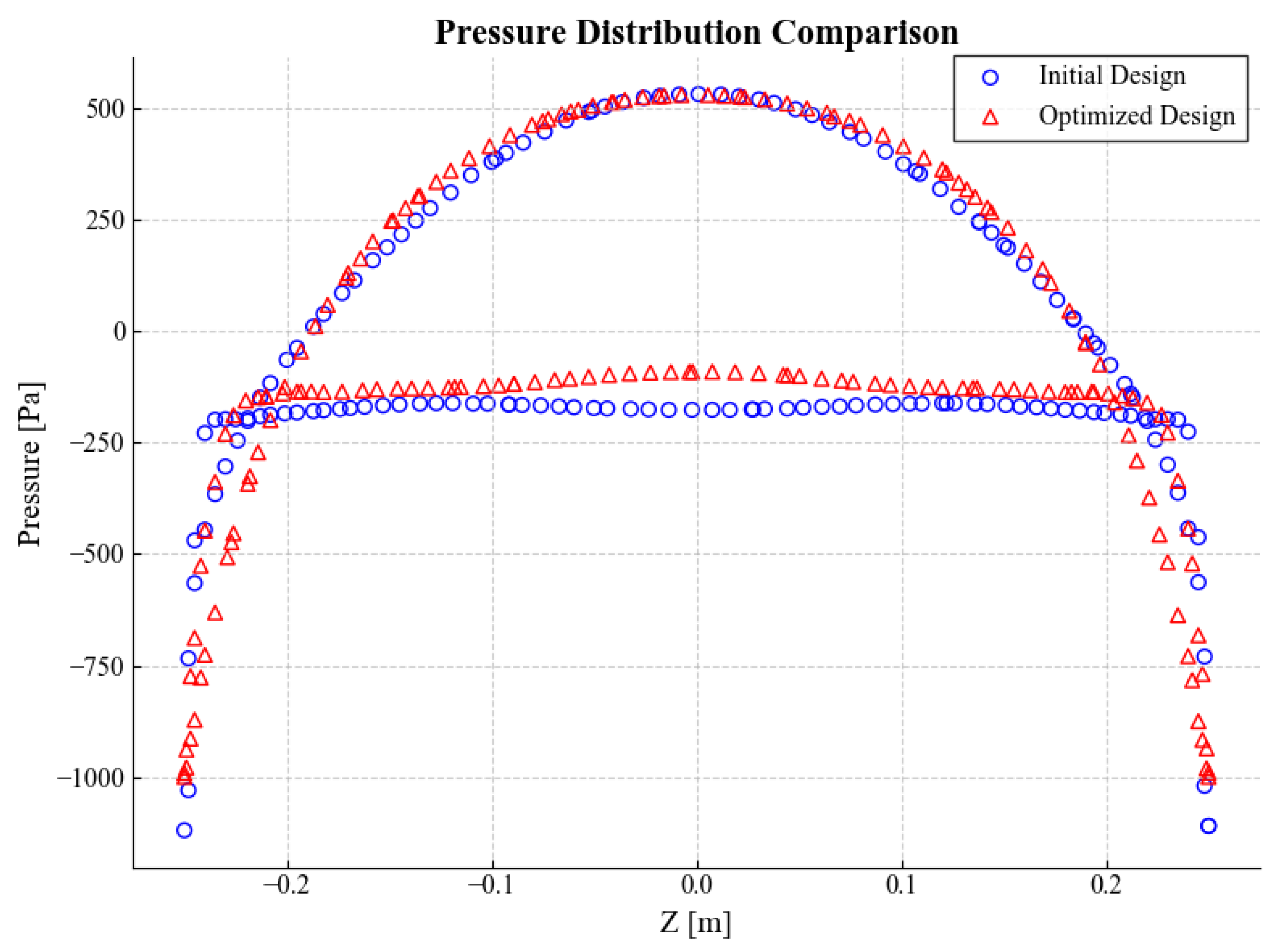
Under vertical motion conditions, the velocity contours presented in Figure 13 illustrate a downward deflection of the wake for both the initial and optimized designs. The initial design generates a diffuse wake, indicating a broad region of energy dissipation. In contrast, the optimized design produces a narrower, more concentrated, and coherent downward jet that extends further downstream. The corresponding pressure contours and quantitative pressure distribution curves are shown in Figure 14 and Figure 15, respectively. A significant pressure differential between the upper and lower hull surfaces is evident in both cases. The optimized design not only achieves a higher pressure peak in the positive pressure region on its upper surface but also enlarges the absolute value of the pressure in the negative pressure zone, thereby effectively increasing the overall pressure differential and directly enhancing lift performance. The pressure distribution on the lower surface shows a reduction in the magnitude of negative pressure compared to the initial design, which helps to suppress the tendency for boundary layer separation. Consequently, the optimized design demonstrates a marked improvement in both hydrodynamic efficiency and navigational stability while generating the required vertical force.

To validate the accuracy of the numerical simulation methodology employed in this study, a comparison is made between the drag coefficients predicted for the optimized design and those obtained directly from numerical computations. The results of this comparison are presented in

Table 11. Comparison of predicted and numerically computed drag coefficients.

Scheme	${\mathit{C}}_{\mathit{dh}}$	${\mathit{C}}_{\mathit{dv}}$
Actual value	0.1632	0.3951
Predicted value	0.1624	0.388
Relative	−0.49%	−1.80%

.

The drag coefficients for both the horizontal and vertical conditions, as predicted by the surrogate model, exhibit strong agreement with the results derived from direct CFD simulations. The relative errors between the predicted and CFD-computed values are merely −0.49% and −1.80%, respectively.

5. Conclusions

This paper presents an efficient and intelligent framework to address the critical challenge of hydrodynamic shape optimization for a novel sea-turtle-inspired AUH. The primary contribution of this work lies not merely in the application of optimization but also in the novel physical insights uncovered through the process. A key scientific finding is the discovery of a distinct discontinuity on the Pareto-optimal front ($C_{dh}\approx [0.20,0.21]$). This phenomenon is interpreted not as an algorithmic artifact, but as a ‘natural gap’ in the performance landscape. Its existence signifies a fundamental design constraint, likely stemming from a critical transition in flow physics or a topological divide between different families of optimal shapes. This insight has immediate practical applications, serving as a crucial guideline for engineers to avoid this suboptimal “forbidden zone,” thereby saving considerable design effort.

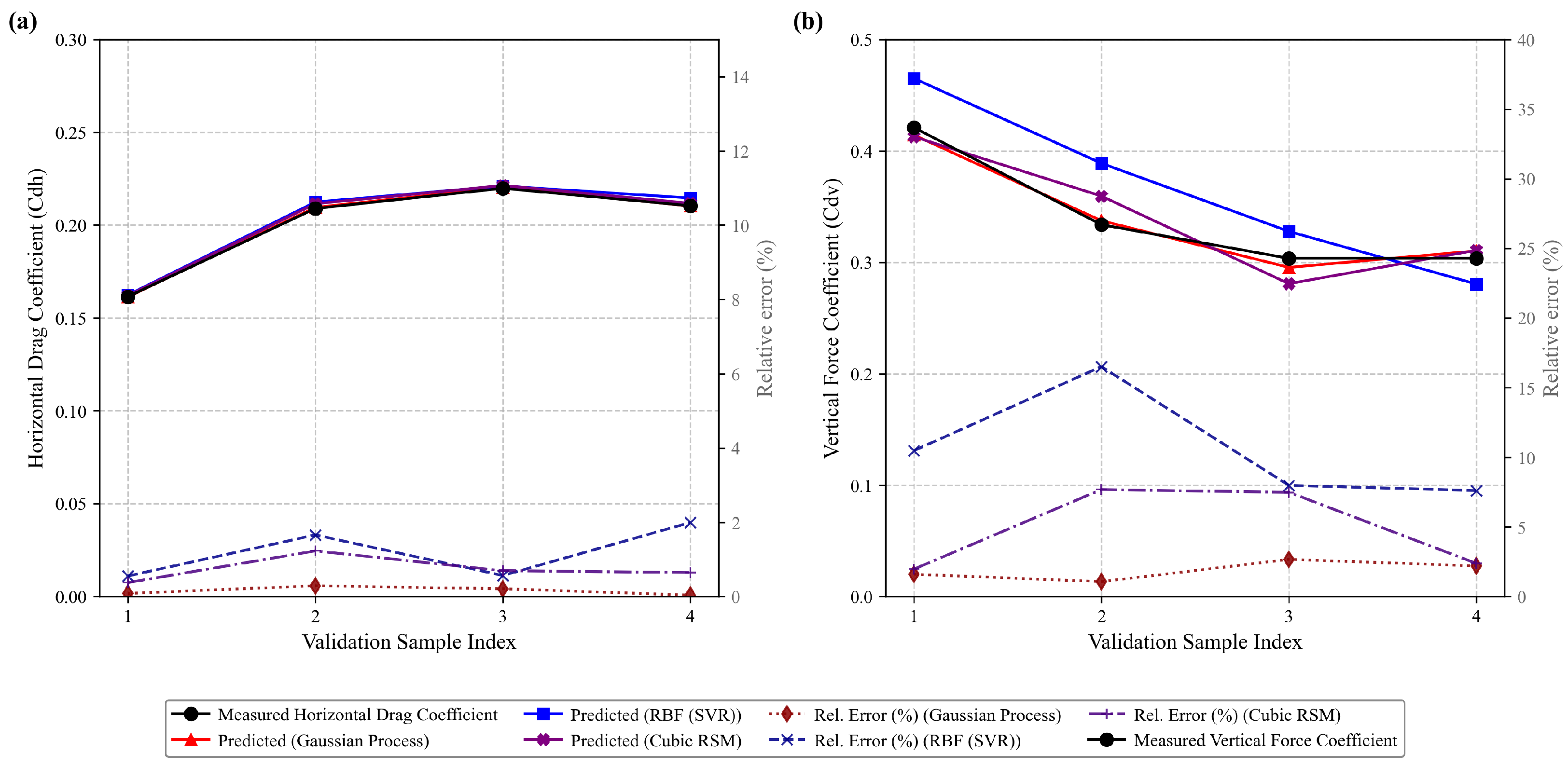
Methodologically, this study demonstrated a robust pathway for complex engineering optimization under tight computational budgets. A non-axisymmetric, bio-inspired AUH hull was first developed by uniquely adapting the Myring equations, governed by two dimensionless shape factors ($n_1$, $n_2$) and integrated into an automated CAD–CFD workflow. To overcome the prohibitive cost of simulations, a high-fidelity GPR surrogate model was constructed from a small 24-point OLHS dataset. The significance of this choice was validated through a direct comparison, where the GPR model’s accuracy (validation R² > 0.98) proved far superior to that of both RBF and Cubic RSM models. Furthermore, the T-NSGA-II algorithm was developed by systematically tuning its hyperparameters with Optuna. Its superior performance was first confirmed on standard ZDT benchmarks and then applied to the AUH problem, where it generated a demonstrably dominant Pareto front compared to the standard NSGA-II.

The integrated framework presented herein—combining parametric modeling, automated analysis, a high-precision surrogate, and a tuned evolutionary algorithm—offers a powerful and transferable methodology. Its application extends to related topics in marine engineering, such as the design of other UUVs or USVs, and could be adapted for complex optimization challenges in the aerospace and automotive sectors.

Future investigations will focus on two key areas: expanding the optimization framework to include additional performance criteria such as hydrodynamic stability and maneuverability, and performing experimental validation of the most promising optimized designs through physical tank testing to verify the predicted performance gains.