An Extended VIKOR-Based Marine Equipment Reliability Assessment Method with Picture Fuzzy Information

Abstract

Reliable operation of marine equipment is crucial for ensuring vessel performance and safeguarding the safety of personnel and the marine environment. However, the complexity of evaluation criteria and the subjectivity inherent in expert judgments pose significant challenges for effective reliability assessment. To address these challenges, this study proposes an extended VIKOR method within a group decision-making (GDM) framework based on picture fuzzy numbers. The method first collects expert evaluations through questionnaires and voting to construct individual decision matrices, and then it applies a newly developed entropy-based approach to determine attribute weights, resulting in a group-weighted decision matrix. Subsequently, an extended VIKOR model is introduced, where the group utility measure is derived from one positive reference matrix and two negative reference matrices, while the group regret measure is based on two negative reference matrices. To improve assessment precision, this study also introduces a novel normalized projection measure to evaluate the closeness between decision matrices. Finally, two ranking strategies are developed, for static and dynamic environments, respectively. The proposed method is validated through a case study on marine equipment reliability assessment, confirming its effectiveness and feasibility. This study provides valuable insights for both theoretical research and practical applications in maritime engineering.

1. Introduction

Vessels often operate in remote maritime areas with limited shore-based support. Reliable operation of onboard equipment is essential for ensuring operational efficiency, crew safety, and protection of the marine environment. Traditionally, marine equipment’s reliability is defined as a system’s ability to perform its intended functions under specified conditions over a given period. In this study, we further refine this definition as the probability of failure-free operation within a defined interval. We focus on two core elements: (1) the watchkeeping practices mandated by the IMO’s International Convention on Standards of Training, Certification, and Watchkeeping for Seafarers (STCW), and (2) the Planned Maintenance System (PMS) frameworks implemented by shipowners and management companies to maintain ongoing regulatory compliance (see [1,2]).

Reliability assessments of marine equipment and systems guide critical decisions on ship design, equipment selection, and vendor evaluation, and they underpin emergency response planning and maintenance scheduling. Consequently, developing robust reliability assessment methodologies has become a central research focus in modern shipping, drawing significant attention from both scholars and industry practitioners.

Several Bayesian and hybrid approaches have been proposed for marine equipment reliability assessment. Toroody et al. [3] combined Bayesian inference with Markov chain Monte Carlo to estimate ship systems’ reliability. Kang et al. [4] developed a hierarchical fault detection and diagnosis framework for engine systems. Xiao et al. [5] integrated probabilistic simulation with experimental data fusion to evaluate local structural reliability in ships. Wang et al. [6] introduced a dynamic Bayesian network merging reverse diagnosis and forward reasoning for subsea mud-lifting system reliability. Bicen et al. [7] formulated the SOHRA (Ship Operator’s Health and Reliability Assessment) model to assess operator reliability during crankshaft replacement. More recently, Chen et al. [8] proposed an algorithm for predictive health monitoring of ship equipment.

Traditional metrics such as mean time between failures (MTBF) and theoretical reliability calculations provide basic estimates for marine equipment. However, they often overlook the combined impacts of human factors, equipment condition, and harsh marine environments—where ships face unique challenges like severe weather, humidity, and salt spray, and lack the maintenance support available to land-based systems. Furthermore, manufacturer data, especially for commercial off-the-shelf (COTS) equipment, typically reflect limited definitions, further constraining reliability assessments. To address these issues, this paper proposes a reliability assessment framework based on actual deployment scenarios, which integrates multidimensional data, better matches the real operational needs of ships, and provides strong support for scientific decision-making by various stakeholders.

Moreover, a complete reliability evaluation must quantify not only the probability of failure but also the potential consequences of failure, including impact severity, repair feasibility under constrained onboard resources, repair duration, economic cost, and human–machine coordination efficiency. For example, shipowners often trade off reliability against operating costs, whereas regulatory bodies such as the Maritime Safety Administration (MSA) and Port State Control (PSC) place greater emphasis on personnel safety and environmental protection. Given the diverse priorities and evaluation criteria of these stakeholders, assessing ship equipment’s reliability is inherently a multi-attribute, group decision-making process.

In multi-attribute decision contexts, engaging multiple decision-makers (DMs) is often essential. Group decision-making (GDM) [9,10] provides a framework for collective evaluation, yet DMs’ differing knowledge, experience, and expertise result in uneven contributions and influence. Consequently, accurately determining each DM’s weight remains a central challenge in GDM research (see [11]).

Entropy, introduced by Shannon [12], quantifies uncertainty within a system. Entropy-based weighting methods viewing the evaluation matrix as an interrelated system have attracted significant attention [13,14]. Wang and Wan [15] proposed a cross-entropy approach for decision-maker weights; Liu et al. [16] developed a socially influenced informational entropy method; Yang et al. [17] formulated a linear programming model; Yang and Pang [18] introduced a cross-entropy measure in a T-spherical fuzzy setting; and Yue [11,19] and He et al. [20] advanced hybrid entropy-based frameworks. Parnell et al. [21] presented a range of entropy-based weighting methods, providing essential theoretical support for determining decision-makers’ weights. However, these existing methods may not fully address the nuances of group decision-making in marine equipment reliability assessment (see Examples 3–4 in Section 5). To address this gap, we propose a novel entropy-based weighting scheme specifically tailored to marine equipment reliability evaluation.

In 1965, Zadeh introduced the concept of fuzzy sets to systematically represent imprecise information in decision-making processes [22]. However, fuzzy sets have inherent limitations in handling higher-order uncertainty. To address this, Atanassov [23,24] extended fuzzy sets to intuitionistic fuzzy sets (IFSs) by introducing membership ($\mu$) and non-membership ($\nu$) degrees constrained such that $\mu +\nu \le 1$, thereby enriching the modeling of vagueness. Xu [25] further developed IFS aggregation operators, but IFSs still cannot fully represent options such as abstention or refusal, as in voting scenarios. To overcome this, Cuong and Kreinovich [26] proposed picture fuzzy sets (PFSs), which incorporate positive ($\mu$), neutral ($\eta$), negative ($\nu$), and refusal ($\pi =1-\mu -\eta -\nu$) membership degrees, enabling the representation of four possible outcomes. Since their introduction, research on PFS similarity measures has further advanced the field of fuzzy decision-making.

Building on picture fuzzy sets (PFSs), Wei [27] first introduced a cosine-based similarity measure using PFSs’ four membership degrees for strategic decision-making. Wei and Gao [28] then proposed a normalized Dice similarity measure with an adjustable parameter for material selection. Luo and Zhang [29] developed a novel PFS similarity metric combining membership, non-membership, and neutral degrees, with applications in pattern recognition and medical diagnosis. Thao [30] conducted a systematic entropy-based evaluation of various PFS similarity measures. Luo et al. [31] presented a relationship-matrix-derived similarity measure for multi-attribute decision tasks. More recently, Ganie and Singh [32] formulated a direct measure operating on all four PFS degrees and embedded it within a new multi-attribute decision-making method.

To the best of our knowledge, picture fuzzy sets (PFSs) have not yet been applied to marine equipment reliability assessment. To fill this gap, we extend PFSs into a shipboard reliability evaluation framework. After reviewing fuzzy information representation techniques and various aggregation operators, we observe that preprocessing or normalization steps inherent to these operators can inadvertently discard critical decision information. To overcome this limitation, we develop a PFS VIKOR framework that bypasses aggregation operators and derives evaluation results directly from raw decision data.

The VIKOR (VlseKriterijumska Optimizacija I Kompromisno Resenje) method [33] is a well-established compromise ranking approach that operates without explicit aggregation operators. It accommodates varying sample sizes and heterogeneous criteria—each with its own weight, interdependence, and potentially conflicting objectives. By simultaneously balancing group utility and group regret measures, VIKOR delivers a decision framework that seeks to maximize overall satisfaction while minimizing collective regret. Moreover, VIKOR’s compromise ranking can group alternatives with similar outcomes into the same rank, aiding decision interpretability.

Marine equipment reliability assessment is highly complex. On the one hand, it requires balancing multiple conflicting objectives, uncertain information, and the potential for catastrophic failures. On the other hand, it involves integrating the perspectives of various stakeholders, including shipowners, classification societies, regulatory authorities, and onboard personnel. Common multi-criteria decision-making (MCDM) methods each have limitations in this context: the Analytic Hierarchy Process (AHP) relies on extensive pairwise comparisons, which become impractical when faced with numerous and conflicting criteria; the Technique for Order of Preference by Similarity to the Ideal Solution (TOPSIS) considers only the distances to ideal and anti-ideal solutions, neglecting “regret” under extreme scenarios and, thus, offering limited value for safety redundancy and risk warning; COPRAS, although able to integrate benefits and costs, does not account for collective regret, which may result in underestimating high-risk equipment; and the Best–Worst Method (BWM), while efficient for weight elicitation, still requires an additional ranking step and provides limited support for dynamic and complex scenarios.

To address these limitations, this study adopts and extends the VIKOR method. VIKOR’s compromise programming framework simultaneously optimizes group utility ($S_i$) and group regret ($R_i$), achieving a dynamic balance between average performance and worst-case risk—an approach well suited to the dual demands for safety and reliability in marine operations. Previous studies [34,35,36,37] have further demonstrated that VIKOR maintains robust ranking stability even under indicator perturbations and fuzzy input conditions. In addition, VIKOR relies only on the normalized $S_i$ and $R_i$ vectors for ranking, allowing for seamless integration with picture fuzzy numbers and the novel projection metric proposed in this paper, without requiring additional aggregation operators.

Extensive research [38] has also demonstrated that the VIKOR method exhibits strong adaptability in a wide range of fuzzy environments. In intuitionistic fuzzy contexts, several GDM models have been developed [39,40,41], while Pythagorean fuzzy extensions further improve decision accuracy [42,43,44]. Interval type-2 fuzzy environments have inspired specialized VIKOR-based frameworks [45,46,47,48], and subsequent work has incorporated linguistic information models into VIKOR-GDM approaches [49,50,51]. Ren et al. [52] proposed a dual-hesitant fuzzy VIKOR method, and Belošević et al. [53] applied VIKOR with triangular fuzzy numbers to early-stage infrastructure evaluation. More recently, Singh and Kumar [54] introduced an integral-based VIKOR technique tailored to complex group decisions, further broadening VIKOR’s application scope.

These approaches have significantly advanced group decision-making research. However, the classical VIKOR method depends on only two reference points—namely, the positive ideal solution (maximum utility matrix) and the negative ideal solution (minimum utility matrix)—which limits its applicability. When additional reference information is available—for example, supplementary datasets, vectors, or matrices—incorporating it into the model allows us to capture richer decision characteristics and address more complex problems.

In this study, we present an extended VIKOR method that integrates multidimensional reference information (supplementary datasets, vectors, and matrices) within a picture fuzzy group decision-making framework to substantially improve the robustness and reliability of evaluation outcomes.

Traditionally, VIKOR employs Euclidean and Hamming distances [55] to assess each alternative’s proximity to the ideal solution; however, the scale-dependent sensitivity of these metrics—where a 1 cm deviation is negligible on a 28 m basketball court but significant for a few-millimeter ant—suggests that adopting a more adaptable proximity measure may improve evaluation precision.

In this work, we replace the conventional Euclidean and Hamming distance measures in the classic VIKOR method with a novel normalized projection metric, thereby refining the decision-making process and providing a more integrated evaluation framework.

Figure 1 shows that the distances between vectors ${\alpha }_1$ and ${\alpha }_2$ and between ${\beta }_1$ and ${\beta }_2$ are both equal to the length of the red vector $\gamma$. In the first case, the two vectors have identical lengths and a small angle ${\theta }_{\alpha }$, whereas in the second case the vectors have identical lengths but are nearly opposite, resulting in a large angle ${\theta }_{\beta }$. Therefore, under equal distances, ${\alpha }_1$ and ${\alpha }_2$ are evidently more similar than ${\beta }_1$ and ${\beta }_2$. Relying solely on distance to assess vector proximity is thus incomplete; angular information should also be considered. Inner product and projection techniques provide a more comprehensive similarity measure (see [19,56,57]).

Group decision-making (GDM) studies that employ projection metrics follow two distinct tracks. Track 1 adopts conventional projection measures: Yue and Jia [58] extended TOPSIS to mixed intuitionistic–fuzzy data by replacing distance with the classic projection metric, Xu and Liu [59] combined interval multiplication with fuzzy preference relations, and Yue [60] used projection-based TOPSIS to rank user satisfaction and loyalty. Track 2 employs standardized projection metrics, whose values are normalized to [0, 1]. Because this range facilitates cross-criterion comparison, interest in standardized projection has increased. Yue and Jia [61] applied it to partner selection with real and interval data, while Jia [62] used it to assess offshore equipment’s reliability. To remedy the incompatibility of traditional projection within TOPSIS-based GDM, Yue [56,63,64] proposed several standardized projection frameworks for software quality evaluation.

A gap remains in that existing projection metrics can be unsuitable in a picture fuzzy setting (see Example 1, Section 4). To close this gap, we have developed a new projection metric that is fully compatible with picture fuzzy sets and yields more reasonable similarity assessments.

Therefore, this study aims to propose a group decision-making framework that integrates picture fuzzy sets, an extended VIKOR method, a standardized projection metric, and an innovative entropy-based weighting scheme, so as to enhance the scientific rigor and objectivity of marine equipment reliability assessment.

The main contributions of this paper are as follows:

(1)

A novel standardized projection metric formula is introduced, enabling the direct assessment of proximity between two picture fuzzy matrices. This development effectively addresses the shortcomings of both classical and standardized projection metrics identified in the existing literature.

(2)

To enhance decision-making accuracy, a weighted geometric mean operator is introduced to calculate the average decision matrix for all participants. Additionally, a method is proposed for determining expert weights based on the proximity between individual decision matrices and the collective average matrix, thus reducing subjectivity and mitigating the dominance of influential authorities.

(3)

By incorporating the projection measure of two picture fuzzy numbers, a complementary matrix is constructed for the maximum evaluation matrix. This results in the generation of three reference matrices for the VIKOR-based group decision-making (GDM) model: one positive and two negative reference matrices for calculating the group utility measure, and two negative reference matrices for determining the group regret measure. By representing the evaluation information as picture fuzzy numbers, we present a novel multi-attribute group decision-making (MAGDM) approach based on the developed VIKOR method, detailing the specific steps for its implementation.

(4)

The proposed extended VIKOR-based GDM method is applied to the reliability assessment of marine equipment. Furthermore, this study introduces new ranking methods tailored for both static and dynamic environments. The effectiveness and advantages of the proposed model are validated through comparisons with existing methods using the same original decision data.

The structure of this paper is as follows: After the Introduction in Section 1, Section 2 details the data collection methods and questionnaire design. Section 3 outlines the fundamental concepts underpinning the study. Section 4 introduces a standardized projection measure. Section 5 describes the weighting method for decision-makers. Section 6 presents the proposed approach for assessing marine equipment reliability. Section 7 applies the method to a case study, demonstrating its effectiveness and providing a discussion based on experimental analysis. Finally, Section 8 concludes the paper and highlights directions for future research.

2. Data Collection

Assessment activities such as tenure reviews and research grant selections are central to professional and scientific practice. As decision problems grow more complex, a single decision-maker (DM) can rarely weigh every relevant factor [65,66,67]; therefore, major choices, ranging from national policy to corporate strategy, now rely on group decision-making. Voting is long-standing and simple, yet each ballot covers only one issue and, thus, conveys limited information. Questionnaires yield richer input, but lengthy item lists or handwritten responses often deter experts due to the extra time and effort involved. In marine equipment reliability assessment, balancing information richness with respondent burden is essential for accurate and efficient data gathering. In light of the limitations of both voting and questionnaire methods, this section will present our data collection and survey design based on the following three principles:

(1)

User Engagement: A high level of participant involvement captures the diverse concerns of ship equipment stakeholders, improves evaluation accuracy, broadens sample representativeness and, consequently, enhances assessment reliability.

(2)

Questionnaire Clarity: A user-friendly, well-organized survey enables respondents to answer quickly and accurately; such clarity encourages participation, minimizes response bias, and increases data reliability.

(3)

Streamlined Data Processing: Efficient post-survey handling avoids information distortion or loss, preserves data integrity, and maximizes analytical value.

To improve evaluation efficiency, we adopt a hybrid approach that combines the simplicity of voting with the information richness of a questionnaire. The questionnaire is the main data collection instrument, and each response is encoded symbolically to provide a structured input format. The complete questionnaire layout appears in

Table 1. Questionnaire design.

$\mathbf{Ship} \mathbf{Equipment}$	Standards
	${\mathit{u}}_1$			${\mathit{u}}_2$			$\cdots$
	✓	◯	✗	✓	◯	✗	✓	◯	✗
$A_1$
$A_2$
$\cdots$

.

Each equipment alternative $(A_1,A_2,A_3,\dots )$ occupies one row of the questionnaire matrix, and each reliability attribute $(u_1,u_2,u_3,\dots )$ occupies one column with three symbolic options. Respondents note their judgment by selecting the appropriate symbol in a cell: (✓) denotes agreement, meaning that the attribute is present or strong; (◯) indicates neutrality or uncertainty; and (✗) signifies disagreement, meaning that the attribute is absent or weak. Blank cells, multiple selections, or unreturned forms are treated as non-responses.

The evaluation experiment was conducted onboard an educational training vessel. This vessel has an overall length of 116 m, a maximum beam of 18 m, a molded depth of 8.35 m, a design draught of 5.4 m, a gross tonnage of 6106 t, and an endurance of approximately 10,000 nmi under unrestricted navigation certification. It is equipped with an advanced integrated bridge system, an AUTO-O class engine-room automation system, a controllable-pitch propeller, shaft and diesel generators, a bow thruster, and a retractable fin stabilizer. Although it lacks cargo holds, the vessel can accommodate up to 196 cadets per voyage, making it an ideal platform for immersive maritime training.

To quantify the group’s preference, we computed a voting percentage, defined as the ratio of “agree” votes to the total number of valid ballots for each option. This metric provides a clear numerical measure of consensus. The complete voting results were presented in picture fuzzy set (PFS) format, which captures agreement, neutrality, and disagreement simultaneously. Using PFSs preserves the full pattern of responses while retaining all information relevant to subsequent decision analysis.

Each decision-maker (DM) assigns a single symbol (✓ for agree, ◯ for neutral, or ✗ for disagree) to every attribute–alternative pair, thereby recording individual evaluations in a concise and uniform manner. The resulting symbolic matrix captures personal preferences while avoiding linguistic ambiguity. Aggregating these entries integrates the panel’s expertise, provides an equitable portrayal of collective priorities, and mitigates bias arising from overly optimistic or pessimistic assessments. Because the three symbols coexist in one structure, the matrix transparently shows the degree of consensus. Full details of the questionnaire design and data collection protocol can be found in Section 7.1.

3. Preliminaries

Definition 1.

A picture fuzzy set (PFS) [26] on a universal set $X$ is defined as $A=\left\{<x,{\mu }_A\left(x\right),{\eta }_A\left(x\right),{\nu }_A\left(x\right)\left|x\in X\right.\right\}$, where ${\mu }_A\left(x\right)$ represents the degree of positive membership, ${\eta }_A\left(x\right)$ denotes the degree of neutrality, and ${\nu }_A\left(x\right)$ corresponds to the degree of negative membership. These parameters satisfy the conditions $0\le {\mu }_A\left(x\right),{\eta }_A\left(x\right),{\nu }_A\le 1$, and $0\le {\mu }_A\left(x\right)+{\eta }_A\left(x\right)+{\nu }_A\left(x\right)\le 1$ for all $x\in X$. Additionally, the refusal degree is determined as ${\pi }_A\left(x\right)=1-{\mu }_A\left(x\right)-{\eta }_A\left(x\right)-{\nu }_A\left(x\right),x\in X$. Notably, when ${\pi }_A\left(x\right)=0$, the PFS reduces to an intuitionistic fuzzy set (IFS) [23]. Furthermore, if both ${\pi }_A\left(x\right)=0$ and ${\eta }_B\left(x\right)=0$, the PFS further simplifies to a conventional fuzzy set [68].

For convenience, Wei [69] called

$$\alpha =\left({\mu }_{\alpha },{\eta }_{\alpha },{\nu }_{\alpha }\right),$$

(1)

a picture fuzzy number (PFN), where $0\le {\mu }_{\alpha },{\eta }_{\alpha },{\nu }_{\alpha }\le 1$, $0\le {\mu }_{\alpha }+{\eta }_{\alpha }+{\nu }_{\alpha }\le 1$, and ${\pi }_{\alpha }+{\mu }_{\alpha }+{\eta }_{\alpha }+{\nu }_{\alpha }=1$.

A picture fuzzy number (PFN) can be effectively illustrated through the following practical scenario: In a democratic election held at a polling station, the council distributes 100 ballots for a specific candidate. The voting outcomes are classified into four distinct categories: “vote for” (30 ballots), “abstain” (50 ballots), “vote against” (10 ballots), and “refusal to vote” (10 ballots). The “abstain” category represents blank ballots, signifying that the voter neither endorses nor opposes the candidate while still participating in the election. Meanwhile, the “refusal to vote” category includes both invalid ballots and cases where voters opted not to cast a vote. These voting results can be mathematically represented as a PFN: $\alpha =\left(0.3, 0.5, 0.1\right)$, where the refusal degree is determined as follows: ${\pi }_{\alpha }=1-0.3-0.5-0.1=0.1$.

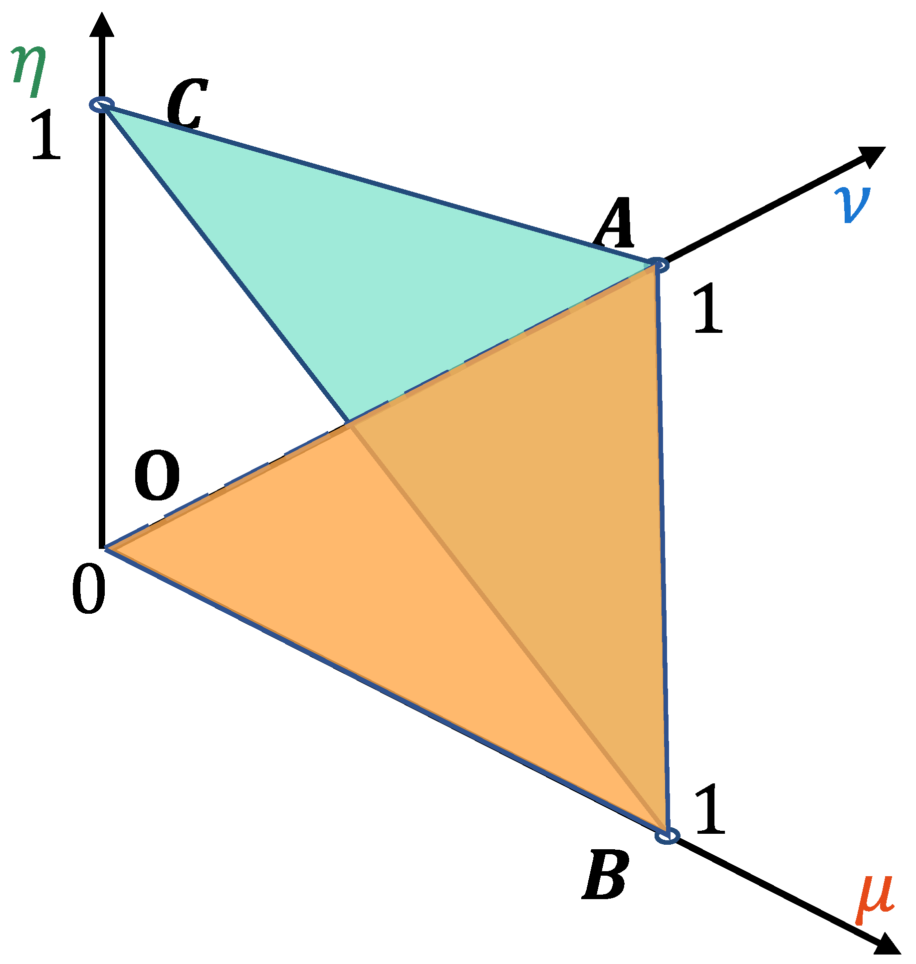
In addition to its numerical formulation, a PFS can be intuitively visualized in the three-dimensional $(\mu ,\eta ,\nu )$ space. Under the above constraints, its feasible domain forms a tetrahedron OABC with vertices at $O(0,0,0)$, $A(1,0,0)$, $B(0,1,0)$, and $C(0,0,1)$. The triangular face OAB (where $\eta =0$) corresponds to the conventional intuitionistic fuzzy set (IFS); when a nonzero neutral membership degree ($\eta >0$) is allowed, the feasible region expands to the entire tetrahedron, as illustrated in Figure 2.

Some operations of PFNs are introduced [69,70] as follows:

Definition 2.

Let $\alpha =\left({\mu }_{\alpha },{\eta }_{\alpha },{\nu }_{\alpha },{\pi }_{\alpha }\right)$ and $\beta =\left({\mu }_{\beta },{\eta }_{\beta },{\nu }_{\beta },{\pi }_{\beta }\right)$ be two PFNs, then

1. 

$\alpha \vee \beta =(\mathit{max}\{{\mu }_{\alpha },{\mu }_{\beta }\},\mathit{min}\{{\eta }_{\alpha },{\eta }_{\beta }\},\mathit{min}\{{\nu }_{\alpha },{\nu }_{\beta }\},\mathit{min}\{{\pi }_{\alpha },{\pi }_{\beta }\})$;

2. 

$\alpha \wedge \beta =(\mathit{min}\{{\mu }_{\alpha },{\mu }_{\beta }\},\mathit{max}\{{\eta }_{\alpha },{\eta }_{\beta }\},\mathit{max}\{{\nu }_{\alpha },{\nu }_{\beta }\},\mathit{max}\{{\pi }_{\alpha },{\pi }_{\beta }\})$;

3. 

$\lambda \alpha =(1-(1-{\mu }_{\alpha }{)}^{\lambda }, ({\eta }_{\alpha }{)}^{\lambda }, ({\eta }_{\alpha }+{\nu }_{\alpha }{)}^{\lambda }-({\eta }_{\alpha }{)}^{\lambda },(1-{\mu }_{\alpha }{)}^{\lambda }-({\eta }_{\alpha }+{\nu }_{\alpha }{)}^{\lambda })(\lambda >0)$;

4. 

${\alpha }^c=({\mu }_{\alpha },{\eta }_{\alpha },{\nu }_{\alpha },{\pi }_{\alpha })$.

Definition 3.

Let $X={\left(x_{ij}\right)}_{m\times n}$ be a matrix, where each element $x_{ij}$ is a picture fuzzy number (PFN). In this context, $X$ is referred to as a picture fuzzy matrix (PFM). Notably, when either $m=1$ or $n=1$, $X$ is designated as a picture fuzzy vector (PFV). For the aggregation of PFNs, Zhang et al. [70] introduced the following operator:

Definition 4.

Let $\tilde{\alpha }=\left({\alpha }_1,\cdots ,{\alpha }_{j,}\cdots ,{\alpha }_n\right)$ be a picture fuzzy vector (PFV), where each element is defined as ${\alpha }_j=\left({\mu }_j,{\eta }_j,{\nu }_j\right)$ for $\left(j=1,2,\dots ,n\right)$. Suppose $w=\left(w_1,\dots ,w_j,\dots ,w_n\right)$ denotes the corresponding weight vector, satisfying $w_j\in \left[0,1\right]$ and ${\sum }_{j=1}^n{w}_j=1$. Then, the picture fuzzy weighted averaging (PFWA) operator is formulated as follows:

$$PFW{A}_{\omega }\left(\tilde{\alpha }\right)=\left(1-{\prod }_{j=1}^n(1-{\mu }_j{)}^{w_j},{\prod }_{j=1}^n({\eta }_j{)}^{w_j},{\prod }_{j=1}^n({\eta }_j+{\nu }_j{)}^{w_j}-{\prod }_{j=1}^n({\nu }_j{)}^{w_j}\right).$$

(2)

Additionally, the PFWA operator can be equivalently expressed as $PFW{A}_{\omega }\left(\tilde{\alpha }\right)={\sum }_{j=1}^n{w}_j{\alpha }_j$.

In particular, if the weight vector is uniformly distributed, i.e., $w=\left({\displaystyle \frac{1}{n}},{\displaystyle \frac{1}{n}},\dots ,{\displaystyle \frac{1}{n}}\right)$, the PFWA operator simplifies to the picture fuzzy arithmetic averaging operator, given by

$$PFW{A}_{\omega }\left(\tilde{\alpha }\right)=\left(1-{\prod }_{j=1}^n(1-{\mu }_j{)}^{{\displaystyle \frac{1}{n}}},{\prod }_{j=1}^n({\eta }_j{)}^{{\displaystyle \frac{1}{n}}},{\prod }_{j=1}^n({\eta }_j+{\nu }_j{)}^{{\displaystyle \frac{1}{n}}}-{\prod }_{j=1}^n({\nu }_j{)}^{{\displaystyle \frac{1}{n}}}\right).$$

(3)

Moreover, Peng et al. [71] introduced a seven-point linguistic rating scale, which establishes a mapping between linguistic variables, corresponding numerical values, and picture fuzzy numbers (PFNs), as summarized in

Table 2. Linguistic variables, corresponding numerical values, and picture fuzzy numbers (PFNs).

Linguistic Variable	Numerical Term	PFN
$\mathrm{Absolutely} \mathrm{Poor} \left(\mathrm{AP}\right)/\mathrm{Absolutely} \mathrm{Low} \left(\mathrm{AL}\right)$	1	$\left(0.00, 0.00, 0.95\right)$
$\mathrm{Very} \mathrm{Poor} \left(\mathrm{VP}\right)/\mathrm{Very} \mathrm{Low} \left(\mathrm{VL}\right)$	2	$\left(0.05, 0.05, 0.85\right)$
$\mathrm{Poor} \left(P\right)/\mathrm{Low} \left(L\right)$	3	$\left(0.10, 0.10, 0.75\right)$
$\mathrm{Fair} \left(F\right)/\mathrm{Medium} \left(M\right)$	4	$\left(0.55, 0.20, 0.20\right)$
$\mathrm{Good} \left(G\right)/\mathrm{High} \left(H\right)$	5	$\left(0.75, 0.10, 0.10\right)$
$\mathrm{Very} \mathrm{Good} \left(\mathrm{VG}\right)/\mathrm{Very} \mathrm{High} \left(\mathrm{VH}\right)$	6	$\left(0.85, 0.05, 0.05\right)$
$\mathrm{Absolutely} \mathrm{Good} \left(\mathrm{AG}\right)/\mathrm{Absolutely} \mathrm{High} \left(\mathrm{AH}\right)$	7	$\left(0.95, 0.00, 0.00\right)$

.

The projection measure plays a pivotal role in evaluating the degree of similarity between different evaluation matrices. In this regard, Wei et al. [72] introduced a projection-based approach to quantify the proximity of one picture fuzzy vector (PFV) to another, as outlined in Definition 5:

Definition 5.

Let $\tilde{\alpha }=\left({\alpha }_1,{\alpha }_2,\dots ,{\alpha }_n\right)$ and $\tilde{\beta }=\left({\beta }_1,{\beta }_2,\dots ,{\beta }_n\right)$ represent two picture fuzzy vectors (PFVs), where ${\alpha }_m=\left({\mu }_{\alpha }^m,{\eta }_{\alpha }^m,{\nu }_{\alpha }^m\right)$ and ${\beta }_m=\left({\mu }_{\beta }^m,{\eta }_{\beta }^m,{\nu }_{\beta }^m\right)$ for $\left(m=1,2,\dots ,t\right)$. The inner product between $\tilde{\alpha }$ and $\tilde{\beta }$ is defined as follows:

$$\tilde{\alpha }\tilde{\beta }={\sum }_{m=1}^t\left({\mu }_{\alpha }^m{\mu }_{\beta }^m+{\eta }_{\alpha }^m{\eta }_{\beta }^m+{\nu }_{\alpha }^m{\nu }_{\beta }^m+{\pi }_{\alpha }^m{\pi }_{\beta }^m\right),$$

(4)

where ${\pi }_{\alpha }^m=1-{\mu }_{\alpha }^m-{\eta }_{\alpha }^m-{\nu }_{\alpha }^m$ and ${\pi }_{\beta }^m=1-{\mu }_{\beta }^m-{\eta }_{\beta }^m-{\nu }_{\beta }^m$, for $m=1,2,\dots ,t$.

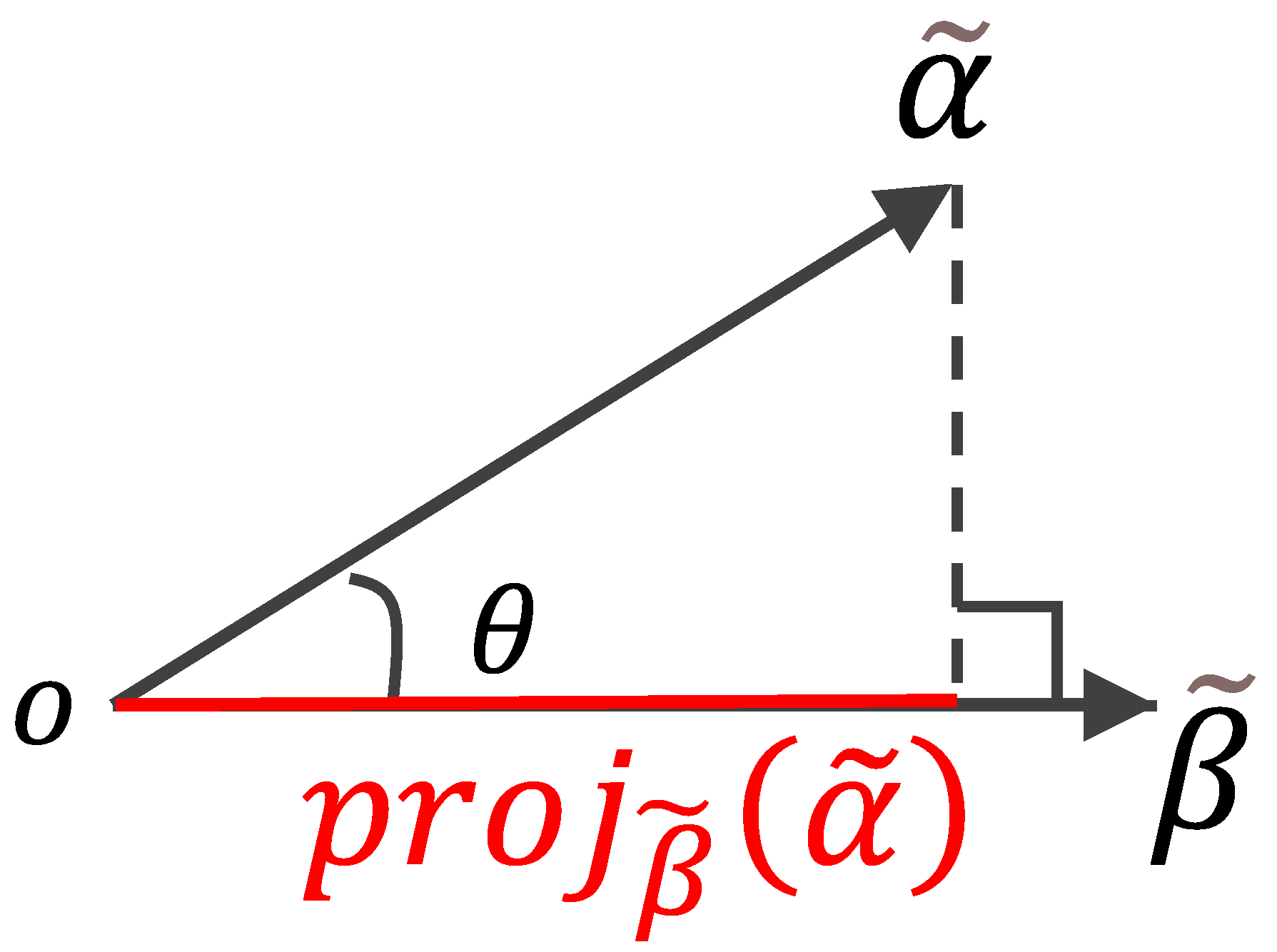
The modulus of $\tilde{\beta }$ is given by

$$\left|\tilde{\beta }\right|=\sqrt{{\sum }_{k=1}^t((}{\mu }_{\beta }^m{)}^2+({\eta }_{\beta }^m{)}^2+({\nu }_{\beta }^m{)}^2+({\pi }_{\beta }^m{)}^2,$$

(5)

The projection of $\tilde{\alpha }$ onto $\tilde{\beta }$, denoted as ${Proj}_{\tilde{\beta }}\left(\tilde{\alpha }\right)$, is defined as follows:

$${Proj}_{\tilde{\beta }}\left(\tilde{\alpha }\right)={\displaystyle \frac{\tilde{\alpha }\tilde{\beta }}{\left|\tilde{\beta }\right|}}.$$

(6)

Figure 3 presents a graphical representation of the projection of $\tilde{\alpha }$ onto $\tilde{\beta }$.

The projection measure, as described in Equation (6), satisfies the following criterion:

Criterion 1.

The greater the value of $Pro{j}_{\tilde{\beta }}\left(\tilde{\alpha }\right)$, the closer $\tilde{\alpha }$ is to $\tilde{\beta }$.

4. Presented Projection Measure

As discussed in the Introduction, projection serves as a fundamental and widely adopted measure for assessing relationships between fuzzy vectors. However, this study uncovers a limitation in its existing formulation, demonstrating that Equation (4) does not consistently adhere to Criterion 1. The following example illustrates this inconsistency:

Example 1.

Let $\tilde{\alpha }=\left(\left(0.850,0.05,0.005\right),\left(0.840,0.06,0.003\right)\right)$ and $\tilde{\beta }=\left(\left(0.710,0.15,0.005\right),\left(0.715,0.18,0.025\right)\right)$ be two picture fuzzy vectors (PFVs). It is evident that $\tilde{\alpha }\ne \tilde{\beta }$. The projection measure is expected to satisfy the condition $Pro{j}_{\tilde{\beta }}\left(\tilde{\beta }\right)>Pro{j}_{\tilde{\beta }}\left(\tilde{\alpha }\right)$. However, applying Equation (4) results in $\tilde{\alpha }\tilde{\beta }=1.2431$, while the norms calculated using Equation (5) are $\left|\tilde{\alpha }\right|=1.2053$ and $\left|\tilde{\beta }\right|=1.0467$. By substituting these values into Equation (6), the projection values are obtained as $Pro{j}_{\tilde{\beta }}\left(\tilde{\alpha }\right)=1.1877$ and $Pro{j}_{\tilde{\beta }}\left(\tilde{\beta }\right)=1.0467$. This outcome, where $Pro{j}_{\tilde{\beta }}\left(\tilde{\beta }\right)<Pro{j}_{\tilde{\beta }}\left(\tilde{\alpha }\right)$, contradicts the expected relationship, highlighting a fundamental inconsistency in the existing projection formulation.

From Example 1, a series of pertinent research questions (RQs) arise:

RQ 1.

The proximity of one picture fuzzy vector (PFV) to another, as determined by Equation (6), does not always adhere to Criterion 1.

RQ 2.

The projection defined in Equation (6) is not a normalized measure. Specifically, it fails to consistently satisfy the condition $0\le Pro{j}_{\tilde{\beta }}\left(\tilde{\alpha }\right)\le 1$. For instance, in Example 1, $Pro{j}_{\tilde{\beta }}\left(\tilde{\alpha }\right)=1.1877$, which exceeds the upper bound of 1.

RQ 3.

The projections $Pro{j}_{\tilde{\alpha }}\left(\tilde{\alpha }\right)$ and $Pro{j}_{\tilde{\beta }}\left(\tilde{\beta }\right)$, as derived from Equation (6), may not be equal. In Example 1, for instance, $\tilde{\alpha }\tilde{\alpha }=1.4527$ based on Equation (4), and $\left|\tilde{\alpha }\right|=1.2053$ according to Equation (5). Consequently, $Pro{j}_{\tilde{\alpha }}\left(\tilde{\alpha }\right)=1.2053$ and $Pro{j}_{\tilde{\beta }}\left(\tilde{\beta }\right)=1.0467$ as calculated from Equation (6), clearly indicating that $Pro{j}_{\tilde{\alpha }}\left(\tilde{\alpha }\right)\ne Pro{j}_{\tilde{\beta }}\left(\tilde{\beta }\right)$.

These observations lead to the following research objectives (ROs):

RO 1.

Develop a projection measure for a PFV $\tilde{\alpha }$ relative to another PFV $\tilde{\beta }$ such that $0\le Pro{j}_{\tilde{\beta }}\left(\tilde{\alpha }\right)\le 1$ for all PFVs.

RO 2.

Ensure that an increase in $Pro{j}_{\tilde{\beta }}\left(\tilde{\alpha }\right)$ corresponds to a closer proximity of $\tilde{\alpha }$ to $\tilde{\beta }$.

RO 3.

Guarantee that $Pro{j}_{\tilde{\alpha }}\left(\tilde{\alpha }\right)=Pro{j}_{\tilde{\beta }}\left(\tilde{\beta }\right)=1$ for all PFVs.

In response to these research questions, a novel projection measure is proposed:

Definition 6.

Let $\tilde{\alpha }=\left({\alpha }_1,{\alpha }_2,\dots ,{\alpha }_n\right)$ and $\tilde{\beta }=\left({\beta }_1,{\beta }_2,\dots ,{\beta }_n\right)$ represent two picture fuzzy vectors (PFVs), where ${\alpha }_m=\left({\mu }_{\alpha }^m,{\eta }_{\alpha }^m,{\nu }_{\alpha }^m\right)$ and ${\beta }_m=\left({\mu }_{\beta }^m,{\eta }_{\beta }^m,{\nu }_{\beta }^m\right)$ for $m=1,2,\dots ,t$. The normalized projection of the vector $\tilde{\alpha }$ onto $\tilde{\beta }$ is defined as follows:

$$MPro{j}_{\tilde{\beta }}\left(\tilde{\alpha }\right)={\displaystyle \frac{\mathit{min}\left\{\left|\tilde{\alpha }\tilde{\beta }\right|,{\left|\tilde{\alpha }\right|}^2,{\left|\tilde{\beta }\right|}^2\right\}}{\mathit{max}\left\{\left|\tilde{\alpha }\tilde{\beta }\right|,{\left|\tilde{\alpha }\right|}^2,{\left|\tilde{\beta }\right|}^2\right\}+\left|1-\frac{\tilde{\alpha }\tilde{\beta }}{{\left|\tilde{\beta }\right|}^2}\right|}},$$

(7)

where $\tilde{\alpha }\tilde{\beta }={\sum }_{m=1}^t({\mu }_{\alpha }^m{\mu }_{\beta }^m+{\eta }_{\alpha }^m{\eta }_{\beta }^m+{\nu }_{\alpha }^m{\nu }_{\beta }^m+{\pi }_{\alpha }^m{\pi }_{\beta }^m)$ represents the inner product between $\tilde{\alpha }$ and $\tilde{\beta }$, ${\left|\tilde{\alpha }\right|}^2={\sum }_{m=1}^t(({\mu }_{\alpha }^m{)}^2+({\eta }_{\alpha }^m{)}^2+({\nu }_{\alpha }^m{)}^2+({\pi }_{\alpha }^m{)}^2)$ is the square of the norm of $\tilde{\alpha }$, and ${\left|\tilde{\beta }\right|}^2={\sum }_{m=1}^t(({\mu }_{\beta }^m{)}^2+({\eta }_{\beta }^m{)}^2+({\nu }_{\beta }^m{)}^2+({\pi }_{\beta }^m{)}^2)$ is the square of the norm of $\tilde{\beta }$. Furthermore, ${\pi }_{\alpha }^m=1-{\mu }_{\alpha }^m-{\eta }_{\alpha }^m-{\nu }_{\alpha }^m$ and ${\pi }_{\beta }^m=1-{\mu }_{\beta }^m-{\eta }_{\beta }^m-{\nu }_{\beta }^m$ for $m=1,2,\dots ,t$.

Criterion 2.

The closer the $MPro{j}_{\tilde{\beta }}(\tilde{\alpha })$ in Equation (7) is to 1, the closer the vector $\tilde{\alpha }$ is to $\tilde{\beta }$.

For instance, consider the picture fuzzy vectors (PFVs) $\tilde{\alpha }=\left(\left(0.850,0.05,0.005\right),\left(0.840,0.06,0.003\right)\right)$ and $\tilde{\beta }=\left(\left(0.710,0.15,0.005\right),\left(0.715,0.18,0.025\right)\right)$ in Example 2. The values are computed as follows: $\left|\tilde{\alpha }\tilde{\beta }\right|=1.2431$, ${\left|\tilde{\alpha }\right|}^2=1.4527$, ${\left|\tilde{\beta }\right|}^2=1.0955$, and $\left|1-{\displaystyle \frac{\tilde{\alpha }\tilde{\beta }}{{\left|\tilde{\beta }\right|}^2}}\right|=0.1347$. The minimum value among $\left\{\left|\tilde{\alpha }\tilde{\beta }\right|,{\left|\tilde{\alpha }\right|}^2,{\left|\tilde{\beta }\right|}^2\right\}$ is $\mathit{min}\left\{1.2431,1.4527,1.0955\right\}=1.0955$, while the maximum value plus the adjustment term gives $\mathit{max}\left\{1.2431,1.4527,1.0955\right\}+0.1347=1.5874$. Hence, the projection of vector $\tilde{\alpha }$ onto $\tilde{\beta }$ is $MPro{j}_{\tilde{\beta }}(\tilde{\alpha })={\displaystyle \frac{1.0955}{1.5874}}=0.6486$. Additionally, since $\tilde{\alpha }\tilde{\alpha }={\left|\tilde{\alpha }\right|}^2$ and $\tilde{\beta }\tilde{\beta }={\left|\tilde{\beta }\right|}^2$, the projection of vector $\tilde{\alpha }$ onto itself is $MPro{j}_{\tilde{\alpha }}(\tilde{\alpha })={\displaystyle \frac{{\left|\tilde{\alpha }\right|}^2}{{\left|\tilde{\alpha }\right|}^2+0}}=1$. Similarly, the projection of $\tilde{\beta }$ onto itself is $MPro{j}_{\tilde{\beta }}(\tilde{\beta })={\displaystyle \frac{{\left|\tilde{\beta }\right|}^2}{{\left|\tilde{\beta }\right|}^2+0}}=1$.

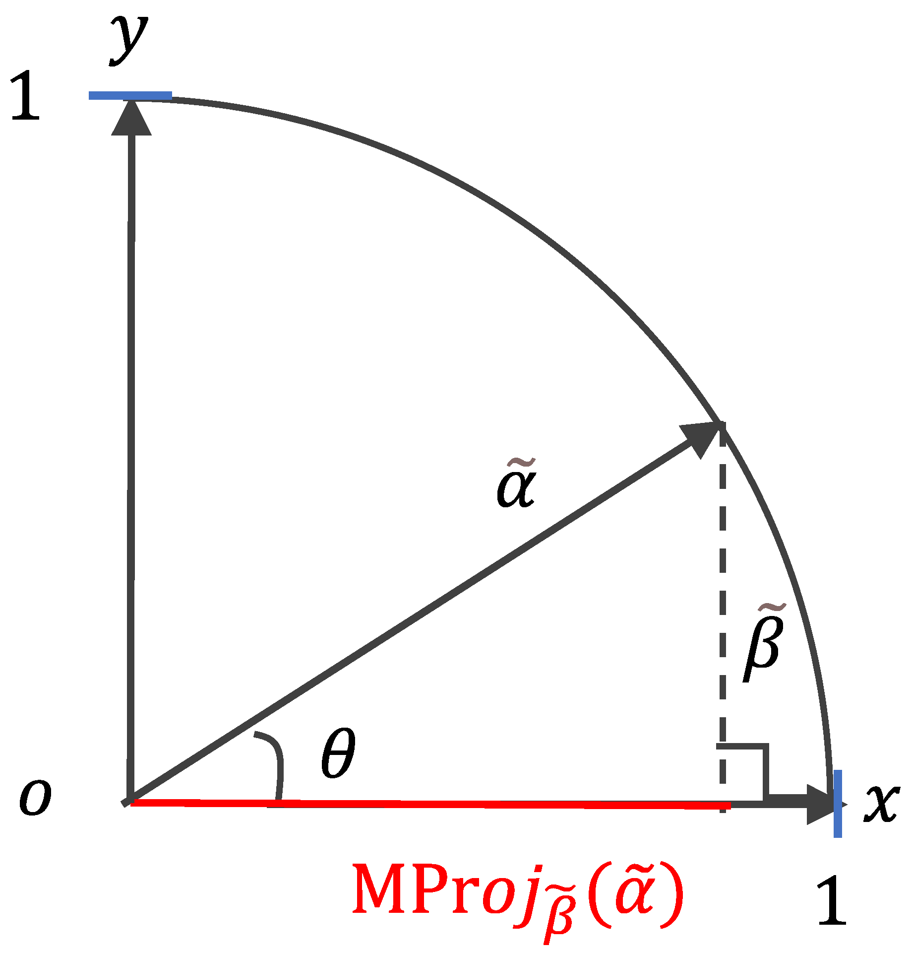
Equation (7) satisfies the criteria set forth in ROs 1–3. As illustrated in Figure 4, the normalized projection value $MPro{j}_{\tilde{\beta }}(\tilde{\alpha })$ is constrained within the interval [0, 1]. The vector $\alpha$ is positioned in the first quadrant, with its endpoint lying on the circumference of a unit circle (radius = 1).

The projection measure defined in Equation (7) is inherently bidirectional, satisfying the condition $MPro{j}_{\tilde{\beta }}\left(\tilde{\alpha }\right)=MPro{j}_{\tilde{\alpha }}\left(\tilde{\beta }\right)$ for any pair of vectors $\tilde{\alpha }$ and $\tilde{\beta }$. A visual depiction of this bidirectional relationship is provided in Figure 5.

Definition 7.

Let $X=(x_{km}{)}_{t\times n}$ and $Y=(y_{km}{)}_{t\times n}$ be two PFMs, where $x_{km}=({\mu }_{km},{\eta }_{km},{\nu }_{km})$, $y_{km}=({\tau }_{km},{\varsigma }_{km},{\upsilon }_{km})(k=1,2\dots ,t;m=1,2\dots ,n)$; then

$$MPro{j}_Y\left(X\right)={\displaystyle \frac{\mathit{min}\left\{XY,{\left|X\right|}^2,{\left|Y\right|}^2\right\}}{\mathit{max}\left\{\left|XY\right|,{\left|X\right|}^2,{\left|Y\right|}^2\right\}+\left|1-\frac{XY}{{\left|Y\right|}^2}\right|}},$$

(8)

is the normalization projection of matrix $X$ onto $Y$, where ${\left|X\right|}^2={\sum }_{k=1}^t{\sum }_{m=1}^n\left(\right({\mu }_{km}{)}^2+({\eta }_{km}{)}^2+({\nu }_{km}{)}^2+({\pi }_{km}{)}^2)$, ${\left|Y\right|}^2={\sum }_{k=1}^t{\sum }_{m=1}^n\left(\right({\tau }_{km}{)}^2+({\varsigma }_{km}{)}^2+({\upsilon }_{km}{)}^2+({\rho }_{km}{)}^2)$, $XY={\sum }_{k=1}^t{\sum }_{m=1}^n({\mu }_{km}{\tau }_{km}+{\eta }_{km}{\varsigma }_{km}+{\nu }_{km}{\upsilon }_{km}+{\pi }_{km}{\rho }_{km})$, and ${\pi }_{km}=1-{\mu }_{km}-{\eta }_{km}-{\nu }_{km}$, ${\rho }_{km}=1-{\tau }_{km}-{\varsigma }_{km}-{\upsilon }_{km}(k=1,2,\dots ,t;m=1,2,\dots ,n)$.

The degree of similarity between two decision matrices, $X$ and $Y$, is assessed according to Criterion 3.

Criterion 3.

The closer the value of $MPro{j}_Y\left(X\right)$ is to 1, the greater the closeness of matrix $X$ to $Y$.

5. A Novel Entropy Measure for Determining Decision Weights

The determination of decision-maker (DM) and attribute weights is a critical component in resolving multi-attribute group decision-making (MAGDM) challenges [73,74,75]. In this study, decision data were collected via structured questionnaires distributed among four expert groups in the maritime industry: ship crew members, technical staff from shipping companies, shipyard maintenance personnel, and regulatory or classification authority representatives such as those from maritime safety administrations (MSAs). Given their varying backgrounds in knowledge, expertise, and practical experience, the influence and contribution of each DM differ. Accordingly, quantifying each DM’s impact—reflected through their assigned weight—remains a key concern in group decision-making (GDM) research (see [11]).

Shannon entropy [11] is a widely used metric for quantifying the degree of disorder within a system, with entropy values increasing as the system becomes more disordered. In multi-criteria decision-making, the decision matrix can be regarded as a decision system, the quality of which can be assessed through an entropy-based approach. Decision-makers (DMs) who provide higher-quality decision matrices, characterized by lower entropy, are assigned greater weights. This highlights the role of entropy as a comprehensive measure for determining the weights of DMs. The relationship between the degree of disorder and entropy is defined as follows:

Criterion 4.

As the level of disorder within a system increases, entropy correspondingly rises; conversely, a higher degree of order results in lower entropy.

The correlation between entropy and the weight assigned to a decision-maker (DM) is defined as follows:

Criterion 5.

A greater entropy value within the evaluation matrix corresponds to a lower weight assigned to the respective DM.

By integrating Criteria 4 and 5, the following principle is established:

Criterion 6.

A DM who provides a more structured and orderly evaluation matrix is assigned a higher weight.

Example 3.

Consider two decision matrices, $N_1$ and $N_2$, provided by decision-makers (DMs) $d_1$ and $d_2$, respectively, as follows:

$$N_1=\begin{array}{ccc}& \begin{array}{ccc}{u}_1& u_2& u_3\end{array}& \\ \begin{array}{c}{A}_1\\ A_2\end{array}& \left(\begin{array}{ccc}AP& AP& AP\\ AP& AP& AP\end{array}\right)& \\ & & \end{array}, N_2=\begin{array}{ccc}& \begin{array}{ccc}{u}_1& u_2& u_3\end{array}& \\ \begin{array}{c}{A}_1\\ A_2\end{array}& \left(\begin{array}{ccc}VG& G& F\\ P& VP& AP\end{array}\right)& \\ & & \end{array},$$

where $A_1$ and $A_2$ represent two alternatives, and $u_1$, $u_2$, and $u_3$ are three benefit attributes (where higher values are preferred), expressed using linguistic variables.

Examining $N_1$, it is evident that all assessment values are categorized as “Absolutely Poor” (AP), indicating a highly structured and uniform evaluation. According to Criterion 6, a well-ordered decision matrix should result in a higher assigned weight for the corresponding DM. However, in this case, DM $d_1$ has provided only “Absolutely Poor” ratings, seemingly without substantive consideration. Consequently, the weight assigned to $d_1$ should, in fact, be significantly lower. This apparent contradiction with Criterion 6 underscores a limitation in the current weighting mechanism.

Similarly, the evaluation values in $N_2$ range from “Very Good” to “Absolutely Poor” in an apparently arbitrary fashion, indicating that DM $d_2$ may not have exercised careful judgment. Consequently, the weight assigned to $d_2$ should be relatively low. However, since the assessment values in $N_2$ are well ordered, Criterion 6 suggests that $d_2$ should be assigned a high weight. This contradiction further underscores an inconsistency in the weighting mechanism.

Example 4 introduces two additional assessment matrices, where $N_1$, $N_2$, $u_1$, $u_2$, and $u_3$ remain consistent with those presented in Example 3. The assessment values in $N_3$ were generated randomly by decision-maker $d_3$ using the MATLAB function $unidrnd$ (7, 2, 3) (MATLAB R2023b). This function produces discrete random numbers drawn from a uniform distribution, with a maximum value of 7, corresponding to the total number of linguistic rating scales specified in Table 2. Parameters 2 and 3 denote the row and column dimensions of the matrix $N_{23}^7$, respectively. The resulting matrix $N_{23}^7$ is shown in Example 4:

Example 4.

$$N_{23}^7=\begin{array}{ccc}& \begin{array}{ccc}{u}_1& u_2& u_3\end{array}& \\ \begin{array}{c}{A}_1\\ A_2\end{array}& \left(\begin{array}{ccc}3& 5& 4\\ 2& 5& 7\end{array}\right)& \\ & & \end{array}, N_3=\begin{array}{c}{A}_1\\ A_2\end{array}\begin{array}{ccc}\begin{array}{ccc}{u}_1& u_2& u_3\end{array}& & \\ \left(\begin{array}{ccc}P& G& F\\ VP& G& AG\end{array}\right)& & \\ & & \end{array}.$$

The numerical values in $N_{23}^7$ are translated into linguistic variables, as shown in matrix $N_3$. It is clear that the assessment values provided by decision-maker $d_3$ seem to be assigned in an arbitrary manner, resulting in a highly disordered set of values. As a result, the weight assigned to $d_3$ should be relatively low.

These anomalies can be analyzed through the entropy values of $N_1$, $N_2$, and $N_3$ in Examples 3 and 4. To support this evaluation, the linguistic variables in $N_1$, $N_2$, and $N_3$ are transformed into picture fuzzy numbers (PFNs), with the conversion method outlined in Table 2. This transformation results in the matrices $M_1$, $M_2$, and $M_3$, as presented below.

$$M_1=\begin{array}{ccc}& \hfill \begin{array}{ccc}\begin{array}{cccccc}\begin{array}{ccc}\hfill \begin{array}{cccc}\hfill \begin{array}{ccccc}\hspace{1em}& \hspace{1em}& \begin{array}{c}{u}_1\end{array}\hfill & & \hspace{1em}\end{array}\hfill & \hspace{1em}& \hspace{1em}& \hfill \begin{array}{ccc} & u_2& \end{array}\hfill \end{array}\hfill & \hspace{1em}& \end{array}& \hspace{1em}& \hspace{1em}& \hfill u_3& \hspace{1em}& \hspace{1em}\end{array}& & \end{array}\hfill & \\ \begin{array}{c}{A}_1\\ A_2\end{array}& \left(\begin{array}{c}\begin{array}{ccc}\left(0.00,0.00,0.95\right)& \left(0.00,0.00,0.95\right)& \left(0.00,0.00,0.95\right)\end{array}\\ \begin{array}{ccc}\left(0.00,0.00,0.95\right)& \left(0.00,0.00,0.95\right)& \left(0.00,0.00,0.95\right)\end{array}\end{array}\right)& \\ & & \end{array},$$

$$M_2=\begin{array}{ccc}& \hfill \begin{array}{ccc}\begin{array}{cccccc}\begin{array}{ccc}\hfill \begin{array}{cccc}\hfill \begin{array}{ccccc}\hspace{1em}& \hspace{1em}& \begin{array}{c}{u}_1\end{array}\hfill & & \hspace{1em}\end{array}\hfill & \hspace{1em}& \hspace{1em}& \hfill \begin{array}{ccc} & u_2& \end{array}\hfill \end{array}\hfill & \hspace{1em}& \end{array}& \hspace{1em}& \hspace{1em}& \hfill u_3& \hspace{1em}& \hspace{1em}\end{array}& & \end{array}\hfill & \\ \begin{array}{c}{A}_1\\ A_2\end{array}& \left(\begin{array}{c}\begin{array}{ccc}\left(0.85,0.05,0.05\right)& \left(0.75,0.10,0.10\right)& \left(0.55,0.20,0.20\right)\end{array}\\ \begin{array}{ccc}\left(0.10,0.10,0.75\right)& \left(0.05,0.05,0.85\right)& \left(0.00,0.00,0.95\right)\end{array}\end{array}\right)& \\ & & \end{array},$$

$$M_3=\begin{array}{ccc}& \hfill \begin{array}{ccc}\begin{array}{cccccc}\begin{array}{ccc}\hfill \begin{array}{cccc}\hfill \begin{array}{ccccc}\hspace{1em}& \hspace{1em}& \begin{array}{c}{u}_1\end{array}\hfill & & \hspace{1em}\end{array}\hfill & \hspace{1em}& \hspace{1em}& \hfill \begin{array}{ccc} & u_2& \end{array}\hfill \end{array}\hfill & \hspace{1em}& \end{array}& \hspace{1em}& \hspace{1em}& \hfill u_3& \hspace{1em}& \hspace{1em}\end{array}& & \end{array}\hfill & \\ \begin{array}{c}{A}_1\\ A_2\end{array}& \left(\begin{array}{c}\begin{array}{ccc}\left(0.10,0.10,0.75\right)& \left(0.75,0.10,0.10\right)& \left(0.55,0.20,0.20\right)\end{array}\\ \begin{array}{ccc}\left(0.05,0.05,0.85\right)& \left(0.75,0.10,0.10\right)& \left(0.95,0.00,0.00\right)\end{array}\end{array}\right)& \\ & & \end{array}.$$

As outlined by Thao [30], the entropy value of a picture fuzzy variable (PFV) is defined as follows:

Definition 8.

Let $\tilde{\alpha }=({\alpha }_1,{\alpha }_2,\dots {\alpha }_t)$ be a PFV, where ${\alpha }_k=({\mu }_{\alpha }^k,{\eta }_{\alpha }^k,{\nu }_{\alpha }^k)(k=1,2,\dots t)$; then

$$E(\tilde{\alpha })=-{\displaystyle \frac{1}{tInt}}{\sum }_{k=1}^t\left({\mu }_{k}In\right({\mu }_k)+{\eta }_{k}In({\eta }_k)+{\nu }_{k}In({\nu }_k)+{\pi }_{k}In({\pi }_k)),$$

(9)

is defined as the entropy of $\tilde{\alpha }$, where ${\pi }_k=1-{\mu }_k-{\eta }_k-{\nu }_k(k=1,2,\dots t)$.

Note: In accordance with Arya and Kumar [76], special cases are addressed as follows: if ${\mu }_k=0$, then ${\mu }_{k}In\left({\mu }_k\right)=0$; if ${\eta }_k=0$, then ${\eta }_{k}In\left({\eta }_k\right)=0$; and if ${\nu }_k=0$, then ${\nu }_{k}In\left({\nu }_k\right)=0$, as specified in Equation (9).

Analogously, the entropy value of a picture fuzzy matrix (PFM) can be defined in an analogous manner:

Definition 9.

Let $X=(x_{km}{)}_{t\times n}$ be a PFM, where $x_{km}=({\mu }_{km},{\eta }_{km},{\nu }_{km})(k=1,2\dots ,t;m=1,2,\dots ,n)$ ; then

$$E(X)=-{\displaystyle \frac{1}{tnIn\left(tn\right)}}{\sum }_{k=1}^t{\sum }_{m=1}^n\left({\mu }_{km}In\right({\mu }_{km})+{\eta }_{km}In({\eta }_{km})+{\nu }_{km}In({\nu }_{km})+{\pi }_{km}In({\pi }_{km})),$$

(10)

is defined as the entropy of $X$, where ${ \pi }_{km}=1-{\mu }_{km}-{\eta }_{km}-{\nu }_{km}(k=1,2\dots ,t;m=1,2,\dots ,n)$.

Special cases are processed according to the conditions outlined in the note to Definition 8.

Based on Equation (10), we can calculate the entropies of $M_1$, $M_2$, and $M_3$ as follows:

$$E\left(M_1\right)=0.8125,E\left(M_2\right)=0.6721,E\left(M_3\right)=0.7603.$$

Let us now revisit the assessment values in $N_1$, $N_2$, and $N_3$, as presented in Examples 3 and 4. In the case of $N_1$, all assessment values are classified as “Absolutely poor.” Correspondingly, the values in matrix $M_1$ remain constant at $\left(0.00,0.00,0.95\right)$. As such, the entropy value $E\left(M_1\right)=0.8125$ is relatively high.

As noted earlier, the assessment values in $N_2$ are similarly well ordered. Consequently, the entropy value $E\left(M_2\right)=0.6721$ is also relatively higher.

Finally, we examine the assessment values in $N_3$, which, as previously mentioned, are randomly assigned by $d_3$. While the entropy value $E\left(M_3\right) = 0.7603$ is deemed acceptable, the corresponding weight, ${\lambda }_3=1-E\left(M_3\right)=1-0.7603=0.2397$, is problematic. This is due to the fact that the assessment values were assigned without careful consideration. Consequently, it is suggested that the weight ${\lambda }_3$ be adjusted to zero.

In conclusion, the rationale for investigating more effective approaches to deriving decision-maker (DM) weights lies in the understanding that, when each decision matrix is appropriately provided (as opposed to being randomly assigned, for instance), the average matrix $M_{\ast }$, along with its corresponding entropy, should more closely align with expectations. If the entropy of a given decision matrix $M_i$ is closer to that of $M_{\ast }$, it suggests that the weight assigned to the respective DM $d_i$ should be greater than that of the other DMs.

In summary, the approach proposed in this study is that the weight assigned to each decision-maker is based on the similarity between the individual decision matrix and the average decision matrix. The average decision matrix is computed using the PFS-weighted arithmetic mean operator. The proximity between the evaluation matrix of the $k$-th decision-maker and the average decision matrix determines the weight assigned to that decision-maker. If the proximity value is higher, it indicates that the evaluation matrix of the expert is more consistent with the average decision matrix, thereby giving more weight to their opinion. As a result, the $k$-th decision-maker is assigned a higher weight. This approach will be implemented in Section 6.

6. Research Methodology

Building on the previously developed framework, this section presents a group decision-making approach based on the VIKOR method, specifically tailored for evaluating the reliability of marine equipment.

The notations presented in

Table 3. Sets and indices.

Set	Index	Description
M	$\{1, 2,\dots ,\left.m\right\}$	Set of evaluated ship equipment indices.
A	$\{A_1,A_2,\dots ,A_i,\dots ,\left.A_m\right\}$	Set of ship equipment indexed by $i\in m$.
N	$\{1, 2,\dots ,\left.n\right\}$	Set of attribute indices.
U	$\{u_1,u_2,\dots ,u_j, \dots ,\left.u_n\right\}$	Set of attributes (evaluation criteria) indexed by $j\in N$.
W	$(w_1, w_2,\dots ,w_j,\dots ,w_n)$	Weight vector of attributes indexed by $j\in N$ with $0\le w_j\le 1$ and ${\sum }_{j=1}^n{w}_j=1.$
T	$\{1, 2,\dots ,\left.t\right\}$	Set of decision-maker indices.
D	$\{d_1, d_2,\dots ,\left.d_k,\dots ,d_t\right\}$	Set of decision-makers, indexed by $k\in t$.

will be employed throughout the model developed in this paper, with the following set of decision-maker (DM) indices:

We assume that the individual decision matrix is formulated by the $k$-th DM $d_k$, as outlined below:

$$M_k=\begin{array}{ccc}& \begin{array}{cccc}{u}_1& u_2& \dots & u_n\end{array}& \\ \begin{array}{c}{P}_1\\ P_2\\ ⋮\\ P_m\end{array}& \left(\begin{array}{cccc}{x}_{11}^k& x_{12}^k& \dots & x_{1n}^k\\ x_{21}^k& x_{22}^k& \dots & x_{2n}^k\\ ⋮& ⋮& ⋮& ⋮\\ x_{m1}^k& x_{m2}^k& \dots & x_{mn}^k\end{array}\right)& \\ & & \end{array}, k\in T,$$

(11)

where $M_k={\left(x_{ij}^k\right)}_{m\times n}$ is the PFM. That is, the attribute values $x_{ij}^k=\left({\mu }_{ij}^k,{\eta }_{ij}^k,v_{ij}^k\right)$ are PFNs for all $i\in M$, $j\in N$, and $k\in T$.

Assuming that $(w_1,w_2,\dots ,w_n)$ denotes the weight vector of the attributes, the corresponding weighted assessment matrices are given by:

$$N_k=\begin{array}{ccc}& \begin{array}{cccc}{u}_1& u_2& \dots & u_n\end{array}& \\ \begin{array}{c}{P}_1\\ P_2\\ ⋮\\ P_m\end{array}& \left(\begin{array}{cccc}{y}_{11}^k& y_{12}^k& \dots & y_{1n}^k\\ y_{21}^k& y_{22}^k& \dots & x_{2n}^k\\ ⋮& ⋮& ⋮& ⋮\\ y_{m1}^k& y_{m2}^k& \dots & y_{mn}^k\end{array}\right)& \\ & & \end{array}, k\in T,$$

(12)

where $N_k=(y_{ij}^k{)}_{m\times n}$ and $y_{ij}^k=w_j\left({\mu }_{ij}^k,{\eta }_{ij}^k,v_{ij}^k\right)=\left({\delta }_{ij}^k,{\iota }_{ij}^k,{\zeta }_{ij}^k\right)=(1-(1-{\mu }_{ij}^k{)}^{w_j},{\left({\eta }_{ij}^k\right)}^{w_j},({\eta }_{ij}^k+v_{ij}^k{)}^{w_j}-{\left({\eta }_{ij}^k\right)}^{w_j})$ based on Equation (2).

In accordance with Equation (3), the arithmetic mean matrix $N_{\ast }$ is defined as follows: For $N_k$ in Equation (12), the arithmetic mean matrix of $N_{\ast }$ (where $k\in T$) is formulated as follows:

$$N_{\ast }=\begin{array}{ccc}& \begin{array}{cccc}{u}_1& u_2& \dots & u_n\end{array}& \\ \begin{array}{c}{P}_1\\ P_2\\ ⋮\\ P_m\end{array}& \left(\begin{array}{cccc}{y}_{11}^{\ast }& y_{12}^{\ast }& \dots & y_{1n}^{\ast }\\ y_{21}^{\ast }& y_{22}^{\ast }& \dots & x_{2n}^{\ast }\\ ⋮& ⋮& ⋮& ⋮\\ y_{m1}^{\ast }& y_{m2}^{\ast }& \dots & y_{mn}^{\ast }\end{array}\right)& \\ & & \end{array}, k\in T,$$

(13)

where $N_{\ast }=(y_{ij}^{\ast }{)}_{m\times n}$ and $y_{ij}^{\ast }=1/t{\sum }_{k=1}^t{y}_{ij}^k=\left({\delta }_{ij}^{\ast },{\iota }_{ij}^{\ast },{\zeta }_{ij}^{\ast }\right)=(1-(1-{{\prod }_{k=1}^t\left({\mu }_{ij}^k\right))}^{1/t}$, ${{\prod }_{k=1}^t\left({\eta }_{ij}^k\right)}^{1/t}$, ${{\prod }_{k=1}^t\left({\eta }_{ij}^k+v_{ij}^k\right)}^{1/t}-{{\prod }_{k=1}^t\left({\eta }_{ij}^k\right)}^{1/t})y_{ij}^{\ast }=1/t{\sum }_{k=1}^t{y}_{ij}^k=\left({\delta }_{ij}^k,{\iota }_{ij}^k,{\zeta }_{ij}^k\right)=(1-(1-{{\prod }_{k=1}^t\left({\mu }_{ij}^k\right))}^{1/t}$, ${{\prod }_{k=1}^t\left({\eta }_{ij}^k\right)}^{1/t}$, ${{\prod }_{k=1}^t\left({\eta }_{ij}^k+v_{ij}^k\right)}^{1/t}-{{\prod }_{k=1}^t\left({\eta }_{ij}^k\right)}^{1/t})$ for all $i\in M$, $j\in N$ [77].

In accordance with Equation (10), the entropy value of $N_k$ is determined as follows:

$$E(N_k)=-{\displaystyle \frac{1}{mnIn\left(mn\right)}}{\sum }_{k=1}^m{\sum }_{j=1}^n({\delta }_{ij}^{k}In({\delta }_{ij}^k)+{\iota }_{ij}^{k}In({\iota }_{ij}^k)+{\zeta }_{ij}^{k}In({\zeta }_{ij}^k)+{\lambda }_{ij}^{k}In({\lambda }_{ij}^k)),$$

(14)

where ${\delta }_{ij}^k$, ${\iota }_{ij}^k$, and ${\zeta }_{ij}^k$ are the same as in Equation (12), ${\lambda }_{ij}^k=1-{\delta }_{ij}^k-{\iota }_{ij}^k-{\zeta }_{ij}^k$, and $0\le E\left(N_k\right)\le 1$ [78].

In accordance with Equation (10), the entropy value of $N_{\ast }$ is determined as follows:

$$E\left(N_{\ast }\right)={\displaystyle \frac{1}{mnIn\left(mn\right)}}{\sum }_{k=1}^m{\sum }_{j=1}^n({\delta }_{ij}^{\ast }In({\delta }_{ij}^{\ast })+{\iota }_{ij}^{\ast }In({\iota }_{ij}^{\ast })+{\zeta }_{ij}^{\ast }In({\zeta }_{ij}^{\ast })+{\lambda }_{ij}^{\ast }In({\lambda }_{ij}^{\ast })), k\in T,$$

(15)

where ${\delta }_{ij}^{\ast }$, ${\iota }_{ij}^{\ast }$, and ${\zeta }_{ij}^{\ast }$ are the same as in Equation (13), ${\lambda }_{ij}^{\ast }=1-{\delta }_{ij}^{\ast }-{\iota }_{ij}^{\ast }-{\zeta }_{ij}^{\ast }$, and $0\le E\left(N_{\ast }\right)\le 1$.

Expanding on the concept outlined in Section 5, we define the following criterion governing the relationship between entropy values and DM weights:

Criterion 10.

As the entropy value $E\left(N_k\right)$ approaches $E\left(N_{\ast }\right)$, the corresponding weight assigned to the DM $d_k$ should increase.

The relative closeness is formulated as follows:

$${\mathit{RC}}_k={\displaystyle \frac{E\left(Y_{\ast }\right)}{E\left(Y_{\ast }\right)+\left|E\left(Y_{\ast }\right)E\left(Y\right)-E{\left(Y_{\ast }\right)}^2\right|}}, k\in T.$$

(16)

The weight attributed to DM $d_k$ is established based on the following criterion:

Criterion 11.

As the relative closeness ${\mathit{RC}}_k$ approaches 1, a higher weight is assigned to DM $d_k$.

In accordance with Criterion 11, the attribute weights ${\phi }_k^{\ast }$ can be defined as follows:

$${\phi }_k^{\ast }={\displaystyle \frac{R{C}_k}{{\sum }_{k=1}^{t}R{C}_k}}, k\in T.$$

(17)

It is evident that ${\phi }_k^{\ast }\ge 0$ and ${\sum }_{k=1}^t{\phi }_k^{\ast }=1$.

The DM weight vector $\Gamma =\left({\phi }_1^{\ast },{\phi }_2^{\ast },\dots ,{\phi }_t^{\ast }\right)$, as defined in Equation (17), facilitates the assignment of ${\phi }_k^{\ast }$ to each corresponding decision $N_k$ in Equation (12). As a result, the individual weighted decision matrix for both attributes and DMs, denoted by $G_k(k\in T)$, is expressed as follows:

$$G_k=\begin{array}{ccc}& \begin{array}{cccc}{u}_1& u_2& \dots & u_n\end{array}& \\ \begin{array}{c}{A}_1\\ A_2\\ ⋮\\ A_m\end{array}& \left(\begin{array}{cccc}{g}_{11}^k& g_{12}^k& \dots & g_{1n}^k\\ g_{21}^k& g_{22}^k& \dots & g_{2n}^k\\ ⋮& ⋮& ⋮& ⋮\\ g_{m1}^k& g_{m2}^k& \dots & g_{mn}^k\end{array}\right)& \\ & & \end{array}, k\in T,$$

(18)

where $g_{ij}^k=\left({\alpha }_{ij}^k,{\beta }_{ij}^k,{\gamma }_{ij}^k\right)=(1-(1-{\delta }_{ij}^k{)}^{{\phi }_k^{\ast }},{\left({\iota }_{ij}^k\right)}^{{\phi }_k^{\ast }},({\iota }_{ij}^k+{\zeta }_{ij}^k{)}^{{\phi }_k^{\ast }}-{\left({\iota }_{ij}^k\right)}^{{\phi }_k^{\ast }})$ according to Definition 2.

To determine the preferential ranking of alternatives, the individual weighted decisions $G_k$ are transformed into a group-weighted decision $P_k\left(i\in M\right)$ for each alternative $A_i$, as follows:

$$P_k=\begin{array}{ccc}& \begin{array}{cccc}{u}_1& u_2& \dots & u_n\end{array}& \\ \begin{array}{c}{d}_1\\ d_2\\ ⋮\\ d_m\end{array}& \left(\begin{array}{cccc}{g}_{11}^i& g_{12}^i& \dots & g_{1n}^i\\ g_{21}^i& g_{22}^i& \dots & g_{2n}^i\\ ⋮& ⋮& ⋮& ⋮\\ g_{t1}^i& g_{t2}^i& \dots & g_{tn}^i\end{array}\right)& \\ & & \end{array}, k\in T,$$

(19)

where $P_k={\left(g_{kj}^i\right)}_{t\times n}$, and the element $g_{kj}^i$ is the same as the element $g_{ij}^k$ in $G_k$ of Equation (18).

According to the idea of the VIKOR technique, the maximal assessment matrix is determined as follows:

$$P_{+}=\begin{array}{ccc}& \begin{array}{cccc}{u}_1& u_2& \dots & u_n\end{array}& \\ \begin{array}{c}{d}_1\\ d_2\\ ⋮\\ d_m\end{array}& \left(\begin{array}{cccc}{g}_{11}^{+}& g_{12}^{+}& \dots & g_{1n}^{+}\\ g_{21}^{+}& g_{22}^{+}& \dots & g_{2n}^{+}\\ ⋮& ⋮& ⋮& ⋮\\ g_{t1}^{+}& g_{t2}^{+}& \dots & g_{tn}^{+}\end{array}\right)& \\ & & \end{array},$$

(20)

where $g_{kj}^{+}=\left({\alpha }_{kj}^{+},{\beta }_{kj}^{+},{\gamma }_{kj}^{+}\right)=\left(ma{x}_{1\le i\le m}\left\{{\alpha }_{kj}^i\right\},mi{n}_{1\le i\le m}\left\{{\beta }_{ij}^k\right\},mi{n}_{1\le i\le m}\left\{{\gamma }_{ij}^k\right\}\right)$ according to Definition 2.

The minimal assessment matrix is defined as follows:

$$P_{-}=\begin{array}{ccc}& \begin{array}{cccc}{u}_1& u_2& \dots & u_n\end{array}& \\ \begin{array}{c}{d}_1\\ d_2\\ ⋮\\ d_m\end{array}& \left(\begin{array}{cccc}{g}_{11}^{-}& g_{12}^{-}& \dots & g_{1n}^{-}\\ g_{21}^{-}& g_{22}^{-}& \dots & g_{2n}^{-}\\ ⋮& ⋮& ⋮& ⋮\\ g_{t1}^{-}& g_{t2}^{-}& \dots & g_{tn}^{-}\end{array}\right)& \\ & & \end{array},$$

(21)

where $g_{kj}^{-}=\left({\alpha }_{kj}^{-},{\beta }_{kj}^{-},{\gamma }_{kj}^{-}\right)=\left(mi{n}_{1\le i\le m}\left\{{\alpha }_{kj}^i\right\},ma{x}_{1\le i\le m}\left\{{\beta }_{ij}^k\right\},ma{x}_{1\le i\le m}\left\{{\gamma }_{ij}^k\right\}\right)$ according to Definition 2.

The complement of $P_{+}$ logically represents an alternative minimal assessment matrix, which is defined as follows:

$$P_c=\begin{array}{ccc}& \begin{array}{cccc}{u}_1& u_2& \dots & u_n\end{array}& \\ \begin{array}{c}{d}_1\\ d_2\\ ⋮\\ d_m\end{array}& \left(\begin{array}{cccc}{g}_{11}^c& g_{12}^c& \dots & g_{1n}^c\\ g_{21}^c& g_{22}^c& \dots & g_{2n}^c\\ ⋮& ⋮& ⋮& ⋮\\ g_{t1}^c& g_{t2}^c& \dots & g_{tn}^c\end{array}\right)& \\ & & \end{array},$$

(22)

where $g_{kj}^c={\left(g_{kj}^{+}\right)}^c=\left({\alpha }_{kj}^{+},{\beta }_{kj}^{+},{\gamma }_{kj}^{+}\right)=\left(mi{n}_{1\le i\le m}\left\{{\alpha }_{kj}^i\right\},ma{x}_{1\le i\le m}\left\{{\beta }_{ij}^k\right\},ma{x}_{1\le i\le m}\left\{{\gamma }_{ij}^k\right\}\right)$ $\left(k\in T,j\in N\right)$ according to Definition 2.

The normalized projection of each group decision $P_i$ on the $P_{+}$, according to Equation (8), is calculated as follows:

$$MPro{j}_{P_{+}}\left(P_i\right)={\displaystyle \frac{min\left\{\left|P_{+}{P}_i\right|,{\left|P_i\right|}^2,{\left|P_{+}\right|}^2\right\}}{max\left\{\left|P_{+}{P}_i\right|,{\left|P_i\right|}^2,{\left|P_{+}\right|}^2\right\}+\left|1-\frac{P_{+}{P}_i}{{\left|P_{+}\right|}^2}\right|}},$$

(23)

where $P_i{P}_{+}={\sum }_{k=1}^t{\sum }_{j=1}^n({\alpha }_{kj}^i{\alpha }_{kj}^{+}+{\beta }_{kj}^i{\beta }_{kj}^{+}+{\gamma }_{kj}^i{\gamma }_{kj}^{+}+{\rho }_{kj}^i{\rho }_{kj}^{+})$, ${\left|P_i\right|}^2={{\sum }_{k=1}^t{\sum }_{j=1}^n(\left({\alpha }_{kj}^i\right)}^2+{\left({\beta }_{kj}^i\right)}^2+{\left({\gamma }_{kj}^i\right)}^2+{\left({\rho }_{kj}^i\right)}^2)$, $\left(i\in M\right)$, ${\left|P_{+}\right|}^2={{\sum }_{k=1}^t{\sum }_{j=1}^n(\left({\alpha }_{kj}^{+}\right)}^2+{\left({\beta }_{kj}^{+}\right)}^2+{\left({\gamma }_{kj}^{+}\right)}^2+{\left({\rho }_{kj}^{+}\right)}^2)$, ${\rho }_{kj}^{+}=1-{\alpha }_{kj}^{+}-{\beta }_{kj}^{+}-{\gamma }_{kj}^{+}$, ${\rho }_{kj}^i=1-{\alpha }_{kj}^i-{\beta }_{kj}^i-{\gamma }_{kj}^i(k\in T,j\in N,i\in M)$.

According to Criterion 3, we have the following Criterion 12:

Criterion 12.

The closer the $MPro{j}_{P_{+}}\left(P_i\right)$ is to 1, and the closer the matrix $P_i$ is to $P_{+}$, the better the ship equipment $A_i$ is.

Similarly, the normalized projection of each group decision $P_i$ on $P_{-}$, according to Equation (8), is calculated as follows:

$$MPro{j}_{P_{-}}\left(P_i\right)={\displaystyle \frac{min\left\{\left|P_{-}{P}_i\right|,{\left|P_i\right|}^2,{\left|P_{-}\right|}^2\right\}}{max\left\{\left|P_{-}{P}_i\right|,{\left|P_i\right|}^2,{\left|P_{-}\right|}^2\right\}+\left|1-\frac{P_{-}{P}_i}{{\left|P_{-}\right|}^2}\right|}},$$

(24)

where $P_i{P}_{-}={\sum }_{k=1}^t{\sum }_{j=1}^n({\alpha }_{kj}^i{\alpha }_{kj}^{-}+{\beta }_{kj}^i{\beta }_{kj}^{-}+{\gamma }_{kj}^i{\gamma }_{kj}^{-}+{\rho }_{kj}^i{\rho }_{kj}^{-})$, ${\left|P_{-}\right|}^2={{\sum }_{k=1}^t{\sum }_{j=1}^n(\left({\alpha }_{kj}^{-}\right)}^2+{\left({\beta }_{kj}^{-}\right)}^2+{\left({\gamma }_{kj}^{-}\right)}^2+{\left({\rho }_{kj}^{-}\right)}^2)$, ${\rho }_{kj}^{-}=1-{\alpha }_{kj}^{-}-{\beta }_{kj}^{-}-{\gamma }_{kj}^{-}(k\in T,j\in N,i\in M)$. The ${\left|P_i\right|}^2$ and ${\rho }_{kj}^i$ are the same as in Equation (23).

The $MPro{j}_{P_{-}}\left(P_i\right)$-based decision criterion is as follows:

Criterion 13.

The closer the $MPro{j}_{P_{-}}\left(P_i\right)$ is to 1, and the closer the matrix $P_i$ is to $P_{-}$, the worse the ship equipment $A_i$ is.

The normalized projection of $P_i$ onto $P_c$, based on Equation (8), is calculated as follows:

$$MPro{j}_{P_c}\left(P_i\right)={\displaystyle \frac{min\left\{\left|P_c{P}_i\right|,{\left|P_i\right|}^2,{\left|P_c\right|}^2\right\}}{max\left\{\left|P_c{P}_i\right|,{\left|P_i\right|}^2,{\left|P_c\right|}^2\right\}+\left|1-\frac{P_c{P}_i}{{\left|P_c\right|}^2}\right|}},i\in M,$$

(25)

where $P_c{P}_i={\sum }_{k=1}^t{\sum }_{j=1}^n({\alpha }_{kj}^i{\alpha }_{kj}^{+}+{\beta }_{kj}^i{\beta }_{kj}^{+}+{\gamma }_{kj}^i{\gamma }_{kj}^{+}+{\rho }_{kj}^i{\rho }_{kj}^{-})$, ${\left|P_c\right|}^2={\left|P_{+}\right|}^2$, ${\rho }_{kj}^c={\rho }_{kj}^{+}$. $P_i$ and ${\rho }_{kj}^i$ are the same as in Equation (23).

The $MPro{j}_{P_c}\left(P_i\right)$-based decision criterion is as follows:

Criterion 14.

The closer the $MPro{j}_{P_c}\left(P_i\right)$ is to 1, and the closer the matrix $P_i$ is to $P_c$, the worse the ship equipment $A_i$ is.

The group utility measure for marine equipment $A_i$ is calculated using the following expression:

$${\mathit{GU}}_i=MPro{j}_{P_{+}}\left(P_i\right)+\lambda MPro{j}_{P_{-}}\left(P_i\right)+\left(1-\lambda \right)MPro{j}_{P_c}\left(P_i\right),i\in M,$$

(26)

where $MPro{j}_{P_{+}}\left(P_i\right)$ is from Equation (23), $MPro{j}_{P_{-}}\left(P_i\right)$ is the same as in Equation (24), $MPro{j}_{P_c}\left(P_i\right)$ is the same as in Equation (25), $\lambda$ is a parameter with $\lambda \in \left[0,1\right]$, $\lambda$ is the weight of $MPro{j}_{P_{-}}\left(P_i\right)$, and $1-\lambda$ is the weight of $MPro{j}_{P_c}\left(P_i\right)$.

The ${\mathit{GU}}_i$-based decision criterion is as follows:

Criterion 15.

The closer the ${\mathit{GU}}_i$ is to 1, the better the ship equipment $A_i$ is.

Inspired by the literature [79], let ${\mathit{GU}}_{max}=ma{x}_{1\le i\le m}\left\{{\mathit{GU}}_i\right\}$, while ${\mathit{GU}}_{min}={min}_{1\le i\le m}\left\{{\mathit{GU}}_i\right\}$. ${\mathit{GU}}_{max}$ is called the largest group utility, while ${\mathit{GU}}_{min}$ is called the smallest group utility. The normalized group utility is defined as follows:

$${\mathit{MGU}}_i=\left\{\begin{array}{c}{\displaystyle \frac{{\mathit{GU}}_i-{\mathit{GU}}_{min}}{{\mathit{GU}}_{max}-{\mathit{GU}}_{min}}},\mathit{if} {\mathit{GU}}_{max}\ne {\mathit{GU}}_{min}\\ 1, \mathit{if} {\mathit{GU}}_{max}={\mathit{GU}}_{min}\end{array}\right.,i\in M,$$

(27)

Based on Criterion 14, we have the following Criterion 16:

Criterion 16.

The closer the ${\mathit{MGU}}_i$ is to 1, the better the ship equipment $A_i$ is.

The group regret measure for marine equipment $A_i$ is defined by the following equation:

$${\mathit{GR}}_i=\chi MPro{j}_{P_{-}}\left(P_i\right)+\left(1-\chi \right)MPro{j}_{P_c}\left(P_i\right),i\in M,$$

(28)

where $MPro{j}_{P_{-}}\left(P_i\right)$ is defined as in Equation (24), and $MPro{j}_{P_c}\left(P_i\right)$ is given as in Equation (25). The parameter $\chi$ lies within the range $\chi \in \left[0,1\right]$. $\chi$ represents the weight of $MPro{j}_{P_{-}}\left(P_i\right)$, while $1-\chi$ corresponds to the weight of $MPro{j}_{P_c}\left(P_i\right)$.

The $G{R}_i$-based decision criterion is as follows:

Criterion 17.

The closer the $G{R}_i$ is to 1, the worse the ship equipment $A_i$ is.

Similar to Equation (28), if we let $G{R}_{max}=ma{x}_{1\le i\le m}\left\{G{R}_i\right\}$, $G{R}_{min}=mi{n}_{1\le i\le m}\left\{G{R}_i\right\}$. The $G{R}_{max}$ is called the smallest group regret, while the $G{R}_{min}$ is called the largest group regret. The normalized group regret of $A_i$ is defined as follows:

$$\begin{array}{c} {\mathit{MGR}}_i=\left\{\begin{array}{c}{\displaystyle \frac{{\mathit{GR}}_{max}-G{R}_i}{{\mathit{GR}}_{max}-{\mathit{GR}}_{min}}},\mathrm{if} {\mathit{GR}}_{max}\ne {\mathit{GR}}_{min}\\ 0, \mathrm{if} {\mathit{GR}}_{max}={\mathit{GR}}_{min}\end{array}\right.,i\in M,\end{array}$$

(29)

Building on Criterion 16, we propose the following:

Criterion 18.

The closer the value of ${\mathit{MGR}}_i$ is to 1, the more preferable the marine equipment $A_i$ becomes.

Accordingly, a comprehensive VIKOR-based measure for equipment $A_i$ can be derived using the following expression:

$$\begin{array}{c} W_i=\beta {\mathit{MGU}}_i+\left(1-\beta \right){\mathit{MGR}}_i,i\in M,\end{array}$$

(30)

where $\beta$ denotes the compromise coefficient, with $\beta \in \left[0,1\right]$. This represents the weight assigned to the normalized group utility ${\mathit{MGU}}_i$, while $1-\beta$ corresponds to the weight of the normalized group regret ${\mathit{MGR}}_i$.

If $\beta >0.5$, it indicates that experts tend to prioritize group utility in their decision-making. Conversely, if $\beta <0.5$, group regret becomes the dominant consideration. When $\beta =0.5$, a balanced and compromise-oriented strategy is adopted. In most cases, $\beta =0.5$ is employed to reflect a neutral stance. By integrating Criteria 16 and 18, we propose the following Criterion 19:

The $W_i$-based decision criterion is as follows:

Criterion 19.

A larger comprehensive relative closeness $W_i$ means the ship equipment $A_i$ is better.

All of the alternatives are ranked by the index $W$. Suppose that $W\left({A_i}^{\left(h\right)}\right)$ denotes the alternative $A_i$ ranked at the $h$th position by $W$ for all $i$, $h= 1, 2,\dots ,m$. This ship $A_i$ is written as $A_{i_h}$ for $W\left({A_i}^{\left(h\right)}\right)$. Now, $m$ alternatives compose a ranking ${A_i}_1\ge {A_i}_2\ge \cdots {A_i}_m$, in descending order.

For two sets of ship equipment ${A_i}_1$ and ${A_i}_2$, if $W\left({A_{i_1}}^{\left(h_1\right)}\right)-W\left({A_{i_2}}^{\left(h_2\right)}\right)<1/\left(m-1\right)$, where $m$ is the quantity of ship equipment, $h_2>h_1$, then we say that the distinction between ${A_i}_1$ and ${A_i}_2$ is small. In this case, the ship equipment $\left\{{A_i}_1,{A_i}_2\right\}$ is classified into the same grade. Beginning with ${A_i}_1$, the ship equipment $\{A_1,A_2,\dots ,A_m\}$ is ranked in phases according to the following procedure:

Phase 1:

If $W\left({A_{i_1}}^{\left(1\right)}\right)-W\left({A_{i_h}}^{\left(h\right)}\right)<1/\left(m-1\right)$ and $W\left({A_{i_1}}^{\left(1\right)}\right)-W\left({A_{i_{\mathrm{h}+1}}}^{\left(h+1\right)}\right)\ge 1/\left(m-1\right)$, where $h\ge 2,$ then the alternatives $\{A_{i_1},A_{i_2},\dots ,A_{i_h}\}$ are considered to be tied for the top rank in the ranking list.

Phase 2:

Starting from $A_{i_{h+1}}$, if $W\left({A_{i_{h+1}}}^{\left(h+1\right)}\right)-W\left({A_{i_h}}^{\left(l\right)}\right)<1/\left(m-1\right)$ and $W\left({A_{i_{\mathrm{h}+1}}}^{\left(h+1\right)}\right)-W\left({A_{i_{l+1}}}^{\left(l+1\right)}\right)\ge 1/\left(m-1\right)$, where $l\ge h+1$, then $\{A_{i_{h+1}},A_{i_{h+2}},\dots ,A_{i_l}\}$ are tied for second place. In this case, a partial order is established as follows:

$$\{A_{i_1},A_{i_2},\dots ,A_{i_h}\}\succ \{A_{i_{h+1}},A_{i_{h+2}},\dots ,A_{i_l}\}.$$

This ranking procedure continues iteratively for the remaining alternatives.

Phase Conclusion: According to the method in Phase 2, the process concludes once $A_{i_m}$ is included in the ranking list.

Procedure for Proposed Approach

Based on the expert voting data described in Section 2 and the attribute definitions pecified in Section 7.1, the proposed method is implemented as follows:

Step 1:

Establish individual decisions.

The individual assessment matrix $M_k={\left(x_{ij}^k\right)}_{t\times n}$ for evaluating the reliability of ship equipment is formulated based on Equation (11), where each element $x_{ij}^k$ is expressed as a picture fuzzy number (PFN). Specifically, $x_{ij}^k=\left({\mu }_{ij}^k,{\eta }_{ij}^k,{\nu }_{ij}^k\right)$, where ${\mu }_{ij}^k$, ${\eta }_{ij}^k$, and ${\nu }_{ij}^k$ denote the degrees of membership, non-membership, and hesitation, respectively, associated with the evaluation provided by the $k$-th DM.

Step 2:

Construction of weighted attribute decision matrices.

Given the attribute weight vector $w_k=\left(w_1,w_2,\dots ,w_n\right)$, the corresponding weighted attribute decision matrix $N_k$ for each DM $k\in T$ is computed in accordance with Equation (12).

Step 3:

Construct the arithmetic mean matrix.

The arithmetic mean matrix $N_{\ast }$, derived from the weighted decision matrices $N_k\left(k\in T\right)$, is constructed in accordance with Equation (13).

Step 4:

Calculation of the entropy values for weighted decisions.

The entropy value $E\left(N_k\right)$ of the weighted decision matrices $N_k$ (where $k\in T$) is computed in accordance with Equation (14).

Step 5:

Calculation of the entropy value for the arithmetic mean matrix.

The entropy value $E\left(N_{\ast }\right)$ of the arithmetic mean matrix $N_{\ast }$ is computed using Equation (15).

Step 6:

Calculation of the relative closeness between the weighted decision entropy and the arithmetic mean matrix entropy.

The relative closeness ${\mathit{RC}}_k$ of the weighted decision entropy $E\left(N_k\right)$ to the entropy value of the arithmetic mean matrix $E\left(N_{\ast }\right)$ is determined using Equation (16).

Step 7:

Determining the DM weights.

The entropy-based weight ${\phi }_k^{\ast }$ for each decision-maker (DM), where $k\in T$, is computed using Equation (17).

Step 8:

Assign DM weights to individual weighted decisions.

The weight ${\phi }_k^{\ast }$ (where $k\in T$) of each DM is applied to the corresponding weighted decision $N_k$ (where $k\in T$). The weighted decision for each DM, $G_k$ (where $k\in T$), is given by Equation (18).

Step 9:

Transformation of individual decision matrices into group decision matrices.

In accordance with Equation (18), the individual decision matrices ${ G}_k$ (where $k\in T$) are transformed into group decision matrices $P_k$ (where $i\in M$), as shown in Equation (19).

Step 10:

Determine the maximum assessment matrix $P_{+}$, the minimum assessment matrix $P_{-}$, and the complement $P_c$ of the maximum assessment matrix.

The maximum assessment matrix $P_{+}$ is calculated using Equation (20). The minimum assessment matrix $P_{-}$ is established according to Equation (21). The complement $P_c$ of the maximum assessment matrix is formed based on Equation (22).

Step 11:

Calculate the normalization projection of $P_i \left(i\in M\right)$ onto $P_{+}$, $P_{-}$, and $P_c$.

The normalization projections $Mpro{j}_{P+}\left(P_i\right) \left(i\in M\right)$, $Mpro{j}_{P_{-}}\left(P_i\right)$, and $Mpro{j}_{P+}\left(P_i\right)$ are calculated using Equations (23), (24), and (25), respectively.

Step 12:

Calculation of the group utility measure.

The group utility $G{U}_i$ is computed based on Equation (26).

Step 13:

Normalization of the group utility.

The normalized group utility $MG{U}_i$ is derived using Equation (27).

Step 14:

Calculation of the group regret measure.

The group regret value ${\mathit{GR}}_i$ is determined as per Equation (28).

Step 15:

Normalization of the group regret.

The normalized group regret $MG{R}_i$ is obtained according to Equation (29).

Step 16:

Compute the comprehensive VIKOR measure.

The comprehensive VIKOR score $W_i$ for the $i$th ship equipment $A_i$ is calculated using Equation (30).

Step 17:

Rank the alternatives.

The alternatives are ranked in descending order according to Criterion 19.

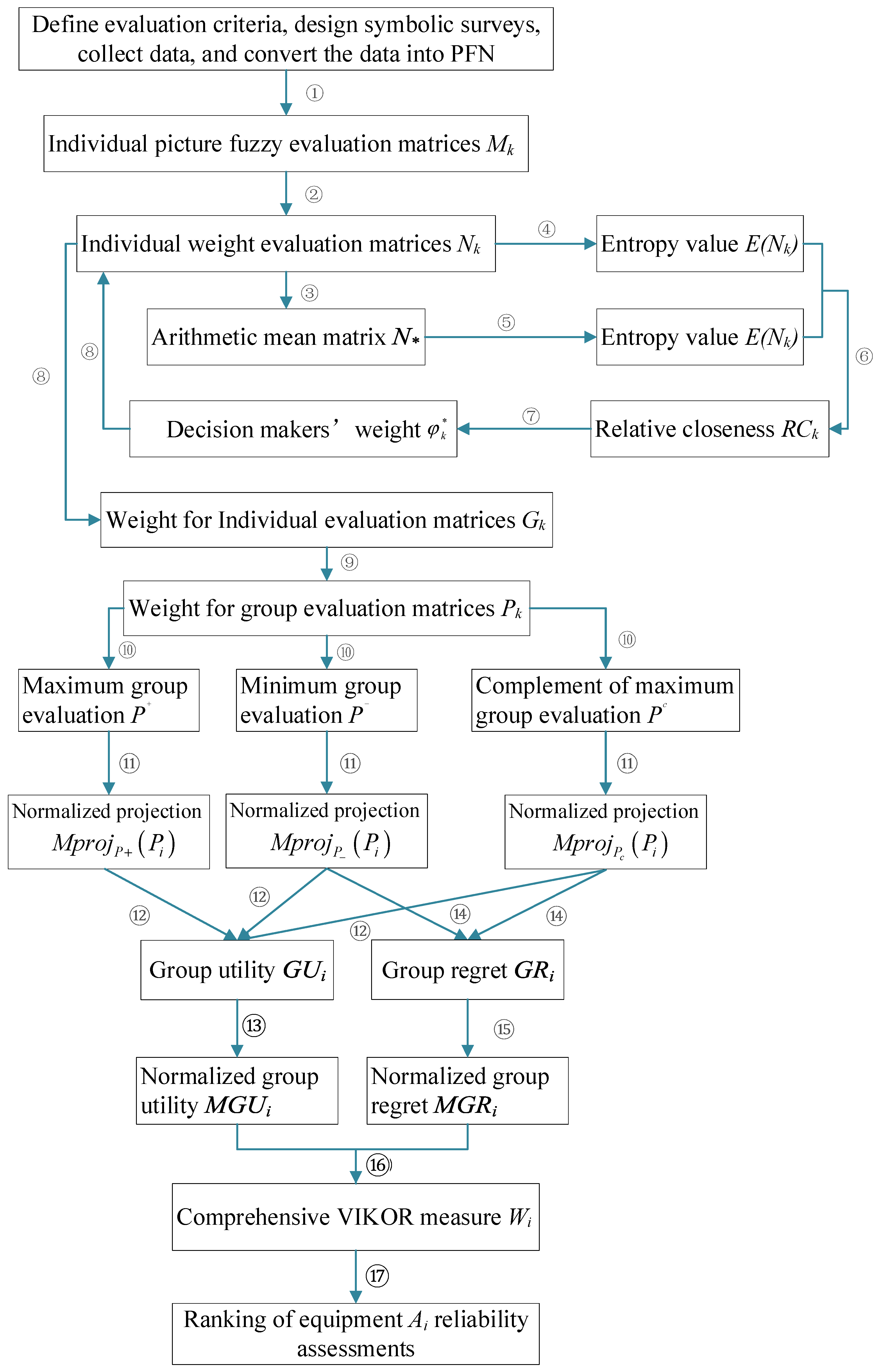
For enhanced clarity, the proposed method’s comprehensive flowchart is presented in Figure 6.

7. Experimental Analysis

7.1. Case Study

This section describes a practical evaluation of the reliability of marine equipment conducted onboard a training vessel operated by a renowned maritime university in Liaoning Province, China. Based on the actual operating environment of the training vessel and expert consultations, three sets of marine equipment were selected as evaluation alternatives, denoted by the set $X=\left\{A_1,A_2,A_3\right\}$. The decision-makers (DMs) comprised four groups of experts with extensive professional backgrounds and practical experience, represented as the set $D=\left\{d_1,d_2,d_3,d_4\right\}$.

$d_1$ (Marine Mechanical Engineering Experts; 100 personnel in total): Graduates in naval architecture and ocean engineering or related fields, experienced in the design, manufacturing, and testing of ships’ mechanical systems, possessing comprehensive expertise in reliability analysis and performance optimization.

$d_2$ (Marine Electrical and Electronic Engineering Experts; 80 personnel in total): Graduates in marine electrical and electronic engineering, proficient in ship automation, power, and control systems, with extensive practical experience in electrical system planning, integration, and fault diagnosis.

$d_3$ (Marine Maintenance Engineering Experts; 77 personnel in total): Graduates in maintenance or reliability engineering, having served as equipment maintenance engineers in shipyards or onboard vessels, skilled in fault diagnosis procedures, maintenance operations, and planning, with practical expertise in equipment lifespan assessment and reliability improvement.

$d_4$ (Maritime Regulatory and Certification Experts; 82 personnel in total): Graduates in maritime management or related fields, employed by the Maritime Safety Administration (MSA) or classification societies, actively involved in formulating and implementing international maritime safety regulations and inspection standards, and specializing in compliance reviews and risk assessments.

This categorization framework effectively integrates the diverse positions and perspectives of stakeholders, ensuring a comprehensive and balanced evaluation process.

The evaluation attribute system was established based on literature review, expert discussions, and practical experience, resulting in four core attributes defined as the set $U=\left\{u_1, u_2, u_3, u_4\right\}=$ {good reputation, low cost, quick repair, easy recovery}, which are detailed as follows:

A good reputation reflects the well-established standing of the equipment or system within the maritime industry, signifying a history of reliable, fault-free performance. Experts assess this attribute based on their professional experience, machinery logs, maintenance records, and other relevant sources. A higher proportion of votes marked with a check (✓) and a lower proportion marked with a cross (✗) or circle (◯) indicate superior performance of this attribute. As such, it is classified as a benefit attribute.

Low cost denotes the relatively minimal financial burden involved in maintaining the reliability of ship equipment or systems, encompassing expenses related to spare parts and materials. Experts assess this attribute based on their professional experience and available inventory of spare parts. As such, low cost is categorized as a benefit attribute.

Rapid repair denotes the minimal time required to restore ship equipment or systems to full operational capacity. This attribute reflects the equipment’s ability to swiftly recover functionality following a failure, which may be enhanced by features such as robust self-diagnostic capabilities or an optimized modular design. As such, this attribute is classified as a benefit factor.

Ease of recovery refers to the capacity of ship equipment or systems to be reinstated with minimal effort following a failure. It reflects the ship’s ability to restore its equipment using only onboard resources and the expertise of the crew, without the need for external support from shipyards or docks. This attribute is therefore classified as a benefit factor.

All of the experts received unified instructions on the evaluation method and scoring criteria before the assessment. They then evaluated the ship equipment according to the defined assessment attributes. The raw scoring data are presented in

Table 4. Original voting statistics.

$\mathbf{DM}$	$\mathbf{Total} \mathbf{Personnel}$	$\mathbf{Ship} \mathbf{Equipment}$	$\mathbf{Voting} \mathbf{for} {\mathit{u}}_1$			$\mathbf{Voting} \mathbf{for} {\mathit{u}}_2$			$\mathbf{Voting} \mathbf{for} {\mathit{u}}_3$			$\mathbf{Voting} \mathbf{for} {\mathit{u}}_4$
			✓	◯	✗	✓	◯	✗	✓	◯	✗	✓	◯	✗
$d_1$	$100$	$A_1$	$49$	$21$	$18$	$50$	$21$	$28$	$46$	$31$	$22$	$42$	$23$	$33$
		$A_2$	$53$	$20$	$12$	$49$	$25$	$25$	$45$	$22$	$32$	$50$	$28$	$18$
		$A_3$	$46$	$19$	$23$	$57$	$09$	$16$	$48$	$14$	$27$	$54$	$21$	$20$
$d_2$	$80$	$A_1$	$29$	$18$	$10$	$34$	$14$	$16$	$30$	$16$	$18$	$41$	$14$	$10$
		$A_2$	$42$	$10$	$17$	$37$	$7$	$13$	$32$	$10$	$22$	$35$	$10$	$9$
		$A_3$	$39$	$9$	$16$	$39$	$8$	$10$	$38$	$3$	$18$	$40$	$7$	$11$
$d_3$	$77$	$A_1$	$35$	$14$	$15$	$42$	$13$	$15$	$35$	$16$	$23$	$40$	$22$	$10$
		$A_2$	$34$	$11$	$18$	$32$	$16$	$13$	$26$	$15$	$22$	$40$	$20$	$16$
		$A_3$	$32$	$13$	$16$	$42$	$5$	$12$	$37$	$11$	$18$	$42$	$14$	$9$
$d_4$	$82$	$A_1$	$40$	$18$	$10$	$42$	$17$	$13$	$38$	$17$	$12$	$36$	$14$	$15$
		$A_2$	$39$	$16$	$13$	$41$	$19$	$8$	$38$	$16$	$11$	$43$	$17$	$9$
		$A_3$	$37$	$15$	$12$	$40$	$16$	$10$	$44$	$15$	$11$	$38$	$18$	$13$

.

In the first step, the evaluation values can be determined by picture fuzzy numbers (PFNs)$\left({\mu }_{ij}^k,{\eta }_{ij}^k,{\nu }_{ij}^k\right)\left(i=1,2,3;j,k=1,2,3,4\right)$ calculated based on the symbolic voting data.

For example, the total number of participants was 100, among whom ${\mu }_{11}^1=49/100=0.49$, ${\eta }_{11}^1=21/100=0.21$, ${\nu }_{11}^1=18/100$. The evaluation matrices for three sets of marine equipment, denoted as $\left\{M_1,M_2,M_3,M_4\right\}$, are presented in

Table 5. Four assessment matrices.

$\mathbf{Matrix}$	$\mathbf{Ship} \mathbf{Equipment}$	${\mathit{u}}_1$	${\mathit{u}}_2$	${\mathit{u}}_3$	${\mathit{u}}_4$
$M_1$	$A_1$	$\left(0.49, 0.21, 0.18\right)$	$\left(0.48, 0.22, 0.27\right)$	$\left(0.46, 0.29, 0.22\right)$	$\left(0.42, 0.23, 0.31\right)$
	$A_2$	$\left(0.52, 0.19, 0.13\right)$	$\left(0.48, 0.25, 0.24\right)$	$\left(0.44, 0.21, 0.31\right)$	$\left(0.49, 0.26, 0.18\right)$
	$A_3$	$\left(0.45, 0.18, 0.24\right)$	$\left(0.56, 0.10, 0.15\right)$	$\left(0.47, 0.12, 0.25\right)$	$\left(0.53, 0.20, 0.19\right)$
$M_2$	$A_1$	$\left(0.36, 0.22, 0.13\right)$	$\left(0.43, 0.18, 0.20\right)$	$\left(0.37, 0.20, 0.23\right)$	$\left(0.51, 0.18, 0.12\right)$
	$A_2$	$\left(0.53, 0.13, 0.21\right)$	$\left(0.46, 0.09, 0.16\right)$	$\left(0.40, 0.13, 0.28\right)$	$\left(0.44, 0.12, 0.11\right)$
	$A_3$	$\left(0.49, 0.11, 0.20\right)$	$\left(0.49, 0.10, 0.12\right)$	$\left(0.48, 0.04, 0.22\right)$	$\left(0.50, 0.09, 0.14\right)$
$M_3$	$A_1$	$\left(0.45, 0.18, 0.20\right)$	$\left(0.54, 0.17, 0.19\right)$	$\left(0.45, 0.21, 0.30\right)$	$\left(0.52, 0.28, 0.13\right)$
	$A_2$	$\left(0.44, 0.14, 0.23\right)$	$\left(0.41, 0.21, 0.17\right)$	$\left(0.34, 0.20, 0.29\right)$	$\left(0.52, 0.26, 0.21\right)$
	$A_3$	$\left(0.41, 0.17, 0.21\right)$	$\left(0.55, 0.07, 0.16\right)$	$\left(0.48, 0.14, 0.23\right)$	$\left(0.54, 0.18, 0.12\right)$
$M_{\ast }$	$A_1$	$\left(0.53, 0.22, 0.13\right)$	$\left(0.52, 0.18, 0.19\right)$	$\left(0.50, 0.19, 0.22\right)$	$(0.48,0.15,0.11)$
	$A_2$	$\left(0.40, 0.19, 0.16\right)$	$\left(0.44, 0.20, 0.10\right)$	$\left(0.39, 0.32, 0.15\right)$	$(0.50,0.08,0.13)$
	$A_3$	$\left(0.47, 0.16, 0.22\right)$	$\left(0.36, 0.06, 0.12\right)$	$\left(0.54, 0.13, 0.23\right)$	$(0.48,0.12,0.12)$

.

Through a negotiation process, the decision-makers (DMs) determine the attribute weights, yielding the weight vector $w=\left(w_1,w_2,w_3,w_4\right)=(0.3,0.2,0.3,0.2)$. In Step 2, the weighted group decisions $N_1$, $N_2$, $N_3$, and $N_4$ are outlined, as shown in

Table 6. Four weighted assessment matrices and their corresponding arithmetic mean matrix.

$\mathbf{Matrix}$	$\mathbf{Ship} \mathbf{Equipment}$	${\mathit{u}}_1$	${\mathit{u}}_2$	${\mathit{u}}_3$	${\mathit{u}}_4$
$N_1$	$A_1$	$\left(0.18, 0.63, 0.13\right)$	$\left(0.12, 0.74, 0.13\right)$	$\left(0.17, 0.69, 0.13\right)$	$(0.10, 0.75, 0.14)$
	$A_2$	$(0.20, 0.61, 0.10)$	$\left(0.12, 0.76, 0.11\right)$	$\left(0.16, 0.63, 0.20\right)$	$\left(0.13, 0.76, 0.08\right)$
	$A_3$	$\left(0.16, 0.60, 0.17\right)$	$\left(0.15, 0.63, 0.13\right)$	$\left(0.17, 0.53, 0.21\right)$	$\left(0.14, 0.72, 0.10\right)$
$N_2$	$A_1$	$\left(0.13, 0.63, 0.09\right)$	$\left(0.11, 0.71, 0.11\right)$	$\left(0.13, 0.62, 0.16\right)$	$\left(0.13, 0.71, 0.08\right)$
	$A_2$	$\left(0.20, 0.54, 0.18\right)$	$\left(0.12, 0.62, 0.14\right)$	$\left(0.14, 0.54, 0.22\right)$	$\left(0.11, 0.65, 0.09\right)$
	$A_3$	$\left(0.18, 0.52, 0.19\right)$	$\left(0.13, 0.63, 0.11\right)$	$\left(0.18, 0.38, 0.29\right)$	$\left(0.13, 0.62, 0.13\right)$
$N_3$	$A_1$	$\left(0.16, 0.60, 0.15\right)$	$\left(0.14, 0.70, 0.11\right)$	$\left(0.16, 0.63, 0.19\right)$	$\left(0.14, 0.78, 0.06\right)$
	$A_2$	$\left(0.16, 0.55, 0.19\right)$	$\left(0.10, 0.73, 0.09\right)$	$\left(0.12, 0.62, 0.19\right)$	$\left(0.14, 0.76, 0.10\right)$
	$A_3$	$\left(0.15, 0.59, 0.16\right)$	$\left(0.15, 0.59, 0.16\right)$	$\left(0.18, 0.55, 0.19\right)$	$\left(0.14, 0.71, 0.08\right)$
$N_4$	$A_1$	$\left(0.20, 0.63, 0.09\right)$	$\left(0.14, 0.71, 0.11\right)$	$\left(0.19, 0.61, 0.16\right)$	$(0.12,0.68,0.08)$
	$A_2$	$\left(0.14, 0.61, 0.12\right)$	$\left(0.11, 0.72, 0.06\right)$	$\left(0.14, 0.71, 0.09\right)$	$\left(0.13, 0.60, 0.13\right)$
	$A_3$	$\left(0.17, 0.58, 0.17\right)$	$\left(0.09, 0.57, 0.14\right)$	$\left(0.21, 0.54, 0.19\right)$	$(0.12,0.65,0.10)$
$N_{\ast }$	$A_1$	$\left(0.17, 0.62, 0.12\right)$	$\left(0.13, 0.71, 0.12\right)$	$\left(0.16, 0.63, 0.16\right)$	$(0.12,0.73,0.09)$
	$A_2$	$\left(0.18, 0.58, 0.15\right)$	$\left(0.11, 0.71, 0.10\right)$	$\left(0.14, 0.62, 0.18\right)$	$(0.13,0.69,0.10)$
	$A_3$	$\left(0.17, 0.57, 0.17\right)$	$\left(0.13, 0.60, 0.13\right)$	$\left(0.18, 0.50, 0.23\right)$	$(0.13,0.68,0.10)$

. Subsequently, the arithmetic mean matrix $N_{\ast }$, derived from all weighted decisions, is established in Step 3. For clarity, the matrix $N_{\ast }$ is also provided in Table 6.

In Step 4, the entropy values $E\left(N_k\right)$ for the weighted matrices $N_k$ (where $k=1,2,3,4$) are computed, with the results presented in Table 6. Step 5 involves the calculation of the entropy value $E\left(N_{\ast }\right)$ for the arithmetic mean matrix $N_{\ast }$, which yields $E\left(N_{\ast }\right)=0.4139$. The relative closeness is determined in Step 6, and in Step 7, the entropy-based weights of the decision-makers (DMs) are derived. The entropy values $E\left(N_k\right)$, relative closeness $R{C}_k(E\left(N_{\ast }\right)=0.4139)$, DMs’ weights ${\phi }_k^{\ast }$, and the corresponding rankings of the DMs are comprehensively summarized in

Table 7. Entropy values $E\left(N_k\right)$, relative closeness ${\mathit{RC}}_k(E\left(N_{\ast }\right)=0.4139)$, DM’s weight ${\phi }_k^{\ast }$, and their ranking.

$$\mathbf{Matrix}$$	$$\mathit{E}\left({\mathit{N}}_{\mathit{k}}\right)$$	$${\mathit{RC}}_{\mathit{k}}$$	$${\mathit{\phi }}_{\mathit{k}}^{\mathit{*}}$$	Ranking
$N_1$	$0.3772$	$0.9646$	$0.2458$	4
$N_2$	$0.4380$	$0.9764$	$0.2488$	3
$N_3$	$0.3947$	$0.9838$	$0.2507$	2
$N_4$	$0.4138$	$0.9999$	$0.2548$	1

.

In Table 7, the decision-makers’ (DMs) weight vector $\left({\phi }_1^{\ast },{\phi }_2^{\ast },{\phi }_3^{\ast },{\phi }_4^{\ast }\right)=\left(0.2458,0.2488,0.2507,0.2548\right)$ is presented. In Step 8, these weights, ${\phi }_k^{\ast }\left(k=1,2,3,4\right)$, are assigned to the individual decisions $N_k$. This results in the weighted decision matrices $G_k\left(k\in T\right)$, which are displayed in

Table 8. Four weighted assessment matrices $G_k\left(k=1,2,3,4\right)$ of three sets of marine equipment.

$${\mathit{G}}_{\mathit{k}}$$	$$\mathbf{Ship} \mathbf{Equipment}$$	$${\mathit{u}}_1$$	$${\mathit{u}}_2$$	$${\mathit{u}}_3$$	$${\mathit{u}}_4$$
$G_1$	$A_1$	$\left(0.05,0.89,0.04\right)$	$\left(0.04,0.93,0.04\right)$	$\left(0.04,0.91,0.04\right)$	$\left(0.03,0.93,0.04\right)$
	$A_2$	$\left(0.05,0.88,0.03\right)$	$\left(0.03,0.93,0.03\right)$	$\left(0.04,0.89,0.06\right)$	$\left(0.03,0.94,0.02\right)$
	$A_3$	$\left(0.04,0.88,0.06\right)$	$\left(0.04,0.89,0.04\right)$	$\left(0.05,0.86,0.07\right)$	$\left(0.04,0.92,0.03\right)$
$G_2$	$A_1$	$\left(0.03,0.89,0.03\right)$	$\left(0.03,0.92,0.03\right)$	$\left(0.03,0.89,0.05\right)$	$\left(0.03,0.92,0.02\right)$
	$A_2$	$\left(0.05,0.86,0.06\right)$	$\left(0.03,0.89,0.05\right)$	$\left(0.04,0.86,0.08\right)$	$\left(0.03,0.90,0.03\right)$
	$A_3$	$\left(0.05,0.85,0.07\right)$	$\left(0.03,0.89,0.04\right)$	$\left(0.05,0.79,0.12\right)$	$\left(0.03,0.89,0.04\right)$
$G_3$	$A_1$	$\left(0.04,0.88,0.05\right)$	$\left(0.04,0.92,0.04\right)$	$\left(0.04,0.89,0.06\right)$	$\left(0.04,0.94,0.02\right)$
	$A_2$	$\left(0.04,0.86,0.07\right)$	$\left(0.03,0.92,0.03\right)$	$\left(0.03,0.89,0.06\right)$	$\left(0.04,0.93,0.03\right)$
	$A_3$	$\left(0.04,0.88,0.05\right)$	$\left(0.04,0.88,0.05\right)$	$\left(0.05,0.86,0.07\right)$	$\left(0.04,0.92,0.02\right)$
$G_4$	$A_1$	$\left(0.06,0.89,0.03\right)$	$\left(0.04,0.92,0.03\right)$	$\left(0.05,0.88,0.05\right)$	$\left(0.03,0.91,0.03\right)$
	$A_2$	$\left(0.04,0.88,0.04\right)$	$\left(0.03,0.92,0.02\right)$	$\left(0.04,0.92,0.03\right)$	$\left(0.03,0.88,0.04\right)$
	$A_3$	$\left(0.05,0.87,0.06\right)$	$\left(0.02,0.87,0.05\right)$	$\left(0.06,0.86,0.07\right)$	$\left(0.03,0.90,0.03\right)$

.

In Step 9, the individual assessment matrices $G_k\left(k=1,2,3,4\right)$ are transformed into the group assessment matrices $P_i\left(i=1,2,3\right)$, as shown in

Table 9. Group assessment matrices of three sets of marine equipment.

${\mathit{P}}_{\mathit{i}}$	$\mathbf{DM}$	${\mathit{u}}_1$	${\mathit{u}}_2$	${\mathit{u}}_3$	${\mathit{u}}_4$
$P_1$	$d_1$	$\left(0.05, 0.89, 0.04\right)$	$\left(0.03, 0.93, 0.04\right)$	$\left(0.04, 0.91, 0.04\right)$	$\left(0.03, 0.93, 0.04\right)$
	$d_2$	$\left(0.05, 0.88, 0.03\right)$	$\left(0.03, 0.93, 0.03\right)$	$\left(0.04, 0.89, 0.06\right)$	$\left(0.03, 0.94, 0.02\right)$
	$d_3$	$\left(0.04, 0.88, 0.06\right)$	$\left(0.04, 0.89, 0.04\right)$	$\left(0.05, 0.86, 0.07\right)$	$\left(0.04, 0.92, 0.03\right)$
	$d_4$	$\left(0.03, 0.89, 0.03\right)$	$\left(0.03, 0.92, 0.03\right)$	$\left(0.03, 0.89, 0.05\right)$	$\left(0.03, 0.92, 0.02\right)$
$P_2$	$d_1$	$\left(0.05, 0.86, 0.06\right)$	$\left(0.03, 0.89, 0.05\right)$	$\left(0.04, 0.86, 0.08\right)$	$\left(0.03, 0.90, 0.03\right)$
	$d_2$	$\left(0.05, 0.85, 0.07\right)$	$\left(0.03, 0.89, 0.04\right)$	$\left(0.05, 0.79, 0.12\right)$	$\left(0.03, 0.89, 0.04\right)$
	$d_3$	$\left(0.04, 0.88, 0.05\right)$	$\left(0.04, 0.92, 0.04\right)$	$\left(0.04, 0.89, 0.06\right)$	$\left(0.04, 0.94, 0.02\right)$
	$d_4$	$\left(0.04, 0.86, 0.07\right)$	$\left(0.03, 0.92, 0.03\right)$	$\left(0.03, 0.89, 0.06\right)$	$\left(0.04, 0.93, 0.03\right)$
$P_3$	$d_1$	$\left(0.04, 0.88, 0.05\right)$	$\left(0.04, 0.88, 0.05\right)$	$\left(0.05, 0.86, 0.07\right)$	$\left(0.04, 0.92, 0.02\right)$
	$d_2$	$\left(0.06, 0.89, 0.03\right)$	$\left(0.04, 0.92, 0.03\right)$	$\left(0.05, 0.88, 0.05\right)$	$\left(0.03, 0.91, 0.03\right)$
	$d_3$	$\left(0.04, 0.88, 0.04\right)$	$\left(0.03, 0.92, 0.02\right)$	$\left(0.04, 0.92, 0.03\right)$	$\left(0.03, 0.88, 0.04\right)$
	$d_4$	$\left(0.05, 0.87, 0.06\right)$	$\left(0.02, 0.87, 0.05\right)$	$\left(0.06, 0.86, 0.07\right)$	$\left(0.03, 0.90, 0.03\right)$

.

Based on Step 10, three reference matrices, $P_{+}$, $P_{-}$, and $P_c$, are established, as shown in

Table 10. Three reference matrices.

$\mathbf{Reference}$	$\mathbf{DM}$	${\mathit{u}}_1$	${\mathit{u}}_2$	${\mathit{u}}_3$	${\mathit{u}}_4$
$P_{+}$	$d_1$	$\left(0.04, 0.88, 0.03\right)$	$\left(0.04, 0.89, 0.03\right)$	$\left(0.05, 0.86, 0.04\right)$	$\left(0.04, 0.92, 0.02\right)$
	$d_2$	$\left(0.05, 0.85, 0.03\right)$	$\left(0.03, 0.89, 0.03\right)$	$\left(0.05, 0.79, 0.05\right)$	$\left(0.03, 0.89, 0.02\right)$
	$d_3$	$\left(0.04, 0.86, 0.05\right)$	$\left(0.04, 0.88, 0.03\right)$	$\left(0.05, 0.86, 0.06\right)$	$\left(0.04, 0.92, 0.02\right)$
	$d_4$	$\left(0.05, 0.87, 0.03\right)$	$\left(0.02, 0.87, 0.02\right)$	$\left(0.06, 0.86, 0.03\right)$	$\left(0.03, 0.88, 0.03\right)$
$P_{-}$	$d_1$	$\left(0.04, 0.89, 0.06\right)$	$\left(0.04, 0.93, 0.04\right)$	$\left(0.05, 0.91, 0.07\right)$	$\left(0.04, 0.94, 0.04\right)$
	$d_2$	$\left(0.05, 0.89, 0.07\right)$	$\left(0.03, 0.92, 0.05\right)$	$\left(0.05, 0.89, 0.12\right)$	$\left(0.03, 0.92, 0.04\right)$
	$d_3$	$\left(0.04, 0.88, 0.07\right)$	$\left(0.04, 0.92, 0.05\right)$	$\left(0.05, 0.89, 0.07\right)$	$\left(0.04, 0.94, 0.03\right)$
	$d_4$	$\left(0.05, 0.89, 0.06\right)$	$\left(0.02, 0.92, 0.05\right)$	$\left(0.06, 0.92, 0.07\right)$	$\left(0.03, 0.91, 0.04\right)$
$P_c$	$d_1$	$\left(0.03, 0.88, 0.04\right)$	$\left(0.03, 0.89, 0.04\right)$	$\left(0.04, 0.86, 0.05\right)$	$\left(0.02, 0.92, 0.04\right)$
	$d_2$	$\left(0.03, 0.85, 0.05\right)$	$\left(0.03, 0.89, 0.03\right)$	$\left(0.05, 0.79, 0.05\right)$	$\left(0.02, 0.89, 0.03\right)$
	$d_3$	$\left(0.05, 0.86, 0.04\right)$	$\left(0.03, 0.88, 0.04\right)$	$\left(0.06, 0.86, 0.05\right)$	$\left(0.02, 0.92, 0.04\right)$
	$d_4$	$\left(0.03, 0.87, 0.05\right)$	$\left(0.02, 0.87, 0.02\right)$	$\left(0.03, 0.86, 0.06\right)$	$\left(0.03, 0.88, 0.03\right)$

.

In Step 11, the normalized projections of each group assessment matrix $P_i$ onto the maximum assessment matrix $P_{+}$, the minimum assessment matrix $P_{-}$, and the complementary assessment matrix $P_c$ are calculated.

The normalization projections and rankings of three sets of marine equipment based on projections are summarized in

Table 11. Normalization projections and their ranking of three sets of marine equipment.

$\mathbf{Ship} \mathbf{Equipment}$	$\mathit{M}\mathit{p}\mathit{r}\mathit{o}{\mathit{j}}_{{\mathit{P}}_{+}}\left({\mathit{H}}_{\mathit{i}}\right)$	$\mathbf{Ranking}$	$\mathit{M}\mathit{p}\mathit{r}\mathit{o}{\mathit{j}}_{{\mathit{P}}_{-}}\left({\mathit{H}}_{\mathit{i}}\right)$	$\mathbf{Ranking}$	$\mathit{M}\mathit{p}\mathit{r}\mathit{o}{\mathit{j}}_{{\mathit{P}}_{\mathit{c}}}\left({\mathit{H}}_{\mathit{i}}\right)$	$\mathbf{Ranking}$
$A_1$	$0.9282$	$3$	$0.9883$	$3$	$0.9282$	$1$
$A_2$	$0.9457$	$2$	$0.9700$	$2$	$0.9457$	$2$
$A_3$	$0.9950$	$1$	$0.9220$	$1$	$0.9950$	$3$

.

Let $\lambda =0.5$, and the group utility values ${\mathit{GU}}_i\left(i=1,2,3\right)$ of marine equipment $A_i\left(i=1,2,3\right)$ are computed in Step 12, based on Equation (26). In Step 13, the normalized group utility values ${\mathit{MGU}}_i\left(i=1,2,3\right)$ are determined using Equation (27). Let $\chi =0.5$, and the group regret values ${\mathit{GR}}_i\left(i=1,2,3\right)$ of marine equipment $A_i$ are calculated in Step 14, according to Equation (28). Step 15 yields the normalized group regret values ${\mathit{MGR}}_i\left(i=1,2,3\right)$ using Equation (29). Let $\beta =0.5$, and the comprehensive VIKOR values $W_i\left(i=1,2,3\right)$ of ships $A_i$ are computed in Step 16, as specified by Equation (30). The VIKOR indices ${\mathit{GU}}_i$, ${\mathit{MGU}}_i$, ${\mathit{GR}}_i$, ${\mathit{MGR}}_i$, and $W_i$, along with the rankings of the three sets of marine equipment, are summarized in

Table 12. VIKOR indices and ranking of three sets of marine equipment.

$\mathbf{Ship}$ $\mathbf{Equipment}$	${\mathit{GU}}_{\mathit{i}}$	$\mathbf{Ranking}$	${\mathit{MGU}}_{\mathit{i}}$	$\mathbf{Ranking}$	${\mathit{GR}}_{\mathit{i}}$	$\mathbf{Ranking}$	${\mathit{MGR}}_{\mathit{i}}$	$\mathbf{Ranking}$	${\mathit{W}}_{\mathit{i}}$	$\mathbf{Ranking}$
$A_1$	$1.8865$	$3$	$0.0000$	$3$	$0.9583$	$2$	$0.3758$	$2$	$0.1879$	$3$
$A_2$	$1.9036$	$2$	$0.2546$	$2$	$0.9579$	$1$	$1.0000$	$1$	$0.6273$	$1$
$A_3$	$1.9535$	$1$	$1.0000$	$1$	$0.9585$	$3$	$0.0000$	$3$	$0.5000$	$2$

.

From Table 12, we can see that $W\left(A_2^{\left(1\right)}\right)-W\left(A_3^{\left(2\right)}\right)=0.6273-0.5000=0.1273$ and $W\left(A_2^{\left(1\right)}\right)-W\left(A_1^{\left(3\right)}\right)=0.6273-0.1879=0.4394$ are both less than $1/(m-1)$ (where $m=3$, so $1/(m-1)=0.5$). According to Step 17, we find that the compromise solutions with classification is $\left\{A_1,A_2,A_3\right\}$. That is, $\left\{A_1,A_2,A_3\right\}$ are in joint first place in the ranking list. According to the traditional rule, the ranking of three marine equipment sets is $A_2>A_3>A_1$. According to the new VIKOR technique, there is no significant difference among the three marine equipment sets. This identification is referred to as one of the VIKOR technique’s advantages.

7.2. Static Analysis

In the experimental analysis presented above, the current model incorporates several evaluation metrics, including $MPro{j}_{P_{+}}\left(P_i\right)$, $MPro{j}_{P_{-}}\left(P_i\right)$, $MPro{j}_{P_c}\left(P_i\right)$, $G{U}_i$, $MG{U}_i$, $G{R}_i$, and $MG{R}_i$. These metrics are individually employed to rank the marine equipment $A_i$, with the ranking process closely resembling the approach used for the comprehensive VIKOR measure $W$.

According to the grading rule defined in Section 6 (Phase 1), the group utility $MPro{j}_{P_{+}}\left(P_i\right)$, as defined in Equation (23), serves as a measure, hereafter referred to as $MPro{j}_{+}$ for convenience. The rankings derived from $MPro{j}_{+}$ are presented in Table 11. Step 11 yields the following values:$MPro{j}_{+}\left(A_3^{\left(1\right)}\right)=0.9950,MPro{j}_{+}\left(A_2^{\left(2\right)}\right)=0.9457,MPro{j}_{+}\left(A_1^{\left(3\right)}\right)=0.9282$. Notably, the difference $MPro{j}_{+}\left(A_3^{\left(1\right)}\right)-MPro{j}_{+}\left(A_1^{\left(3\right)}\right)=0.9950-0.9282=0.0668<{\displaystyle \frac{1}{2}}$ is less than $1/\left(m-1\right)$, implying that the three alternatives $\left\{A_1,A_2,A_3\right\}$ must be classified into the same grade based on the $MPro{j}_{+}$ measure.

Similar to the results obtained with $MPro{j}_{+}$, the application of the measures $MPro{j}_{-}$, $MPro{j}_c$, $GU$, and $GR$ also leads to the classification of three sets of marine equipment into a single grade.

The three sets of marine equipment are assigned to a single grade based on the five aforementioned measures. This outcome is due to the minimal differences observed in the measured values. To mitigate this limitation, the values of the measures are normalized using Equation (27) and Equation (29), respectively.

From Table 12, we can see that $MGU\left(A_3^{\left(1\right)}\right)=1.0000$, $MGU\left(A_2^{\left(2\right)}\right)=0.2546$, $MGU\left(A_1^{\left(3\right)}\right)=0$. From the difference, $MGU\left(A_3^{\left(1\right)}\right)-MGU\left(A_2^{\left(2\right)}\right)=1.0000-0.2546=0.7454>{\displaystyle \frac{1}{2}}$, and $MGU\left(A_2^{\left(2\right)}\right)-MGU\left(A_1^{\left(3\right)}\right)=0.2546-0=0.2546<{\displaystyle \frac{1}{2}}$, so we have $A_3>\left\{A_1,A_2\right\}$ according to the measure $MGU$.

If the regret measure $G{R}_i$ is normalized, then the $MG{R}_i$ in Table 12 shows that $MGR\left(A_2^{\left(1\right)}\right)=1.0000$, $MGR\left(A_1^{\left(2\right)}\right)=0.3758$, $MGR\left(A_3^{\left(3\right)}\right)=0$. From the difference $MGR\left(A_2^{\left(1\right)}\right)-MGR\left(A_1^{\left(2\right)}\right)=1.0000-0.3758=0.6242>{\displaystyle \frac{1}{2}}$ and $MGR\left(A_1^{\left(2\right)}\right)-MGR\left(A_3^{\left(3\right)}\right)=0.3758-0=0.3758<{\displaystyle \frac{1}{2}}$, we know that $A_2>\left\{A_1,A_3\right\}$ according to the measure $MGR$.

The rankings with classification based on the measures $MPro{j}_{+}$, $MPro{j}_{-}$, $MPro{j}_c$, $GU$, $MGU$, $GR$, and $MGR$ $W$ are summarized in

Table 13. Rankings with classification based on the measures.

Measure	${\mathit{A}}_1$	${\mathit{A}}_2$	${\mathit{A}}_3$	$\mathbf{Ranking} \mathbf{with} \mathbf{Classification}$
$MPro{j}_{+}$	✓	✓	✓	$\left\{A_1,A_2,A_3\right\}$
$MPro{j}_{-}$	✓	✓	✓	$\left\{A_1,A_2,A_3\right\}$
$MPro{j}_c$	✓	✓	✓	$\left\{A_1,A_2,A_3\right\}$
$GU$	✓	✓	✓	$\left\{A_1,A_2,A_3\right\}$
$MGU$			✓	$A_3>\left\{A_1,A_2\right\}$
$GR$	✓	✓	✓	$\left\{A_1,A_2,A_3\right\}$
$MGR$		✓		$A_2>\left\{A_1,A_3\right\}$
$W$	✓	✓	✓	$\left\{A_1,A_2,A_3\right\}$
$\mathrm{S}\mathrm{u}\mathrm{m}\mathrm{m}\mathrm{a}\mathrm{r}\mathrm{y}$	6	7	7	$\left\{A_2,A_3\right\}>A_1$

.

It can be observed from Table 13 that the ranking of the three sets of marine equipment is $\left\{A_2,A_3\right\}>A_1$. In other words, $A_2$ and $A_3$ are tied for first place, followed by $A_1$.

7.3. Comparison with a Different VIKOR-Based GDM Approach

As introduced by Yue [80], the group utility measure is defined as follows:

$$\begin{array}{c} S_i={\displaystyle \frac{Mpro{j}_{P_{+}}\left(P_i\right)}{Mpro{j}_{P_{+}}\left(P_i\right)+Mpro{j}_{P_{+}}\left(P_{-}\right)}},i\in M, \end{array}$$

(31)

where $MPro{j}_{P_{+}}\left(P_i\right)$ is the same as defined in Equation (23). The authors of [80] defined the group regret for marine equipment $A_i$ as follows:

$$\begin{array}{c} R_i=1-S_i,i\in M,\end{array}$$

(32)

where $S_i$ is specified as shown in Equation (31).

If the group utility measure is redefined according to Equation (32), the comprehensive VIKOR index $W_i$ is subsequently modified as follows:

$$\begin{array}{c}{W_i}^{\left(2\right)}=\beta {{\mathit{MGU}}_i}^{\left(2\right)}+\left(1-\beta \right){{\mathit{MGR}}_i}^{\left(2\right)},i\in M,\end{array}$$

(33)

where ${\mathit{MGU}}_i^{\left(2\right)}={\displaystyle \frac{\left(S_i-S_{min}\right)}{\left(S_{max}-S_{min}\right)}}$, $S_{max}={max}_{1\le i\le m}\left\{S_i\right\}$, $S_{min}={min}_{1\le i\le m}\left\{S_i\right\}$. ${\mathit{MGR}}_i^{\left(2\right)}=\left(R_i-R_{min}\right)/\left(R_{max}-R_{min}\right)$, $R_{max}={max}_{1\le i\le m}\left\{R_i\right\}$, $R_{min}={min}_{1\le i\le m}\left\{R_i\right\}$.

The subsequent experimental data are likewise derived from the illustrative example presented in Section 7.1.

The measurements derived from the VIKOR indices, namely, $S_i^{\left(2\right)}$, ${\mathit{MGU}}_i^{\left(2\right)}$, $R_i^{\left(2\right)}$, ${\mathit{MGR}}_i^{\left(2\right)}$, and $W_i^{\left(2\right)}$, along with the precise rankings of the three sets of marine equipment, are presented in

Table 14. VIKOR indices and rankings for the three sets of marine equipment calculated using the approach from [74].

$\mathbf{Ship}$ $\mathbf{Equipment}$	${\mathit{S}}_{\mathit{i}}^{\left(2\right)}$	$\mathbf{Ranking}$	${\mathit{MGU}}_{\mathit{i}}^{\left(2\right)}$	$\mathbf{Ranking}$	${\mathit{R}}_{\mathit{i}}^{\left(2\right)}$	$\mathbf{Ranking}$	${\mathit{MGR}}_{\mathit{i}}^{\left(2\right)}$	$\mathbf{Ranking}$	${\mathit{W}}_{\mathit{i}}^{\left(2\right)}$	$\mathbf{Ranking}$
$A_1$	$0.4843$	$3$	$0.0000$	$3$	$0.5157$	$3$	$0.0000$	$3$	$0.0000$	$3$
${\mathrm{A}}_2$	$0.4937$	$2$	$0.2689$	$2$	$0.5063$	$2$	$0.2689$	$2$	$0.2689$	$2$
$A_3$	$0.5190$	$1$	$1.0000$	$1$	$0.4810$	$1$	$1.0000$	$1$	$1.0000$	$1$

.

Table 14 shows that the differences of measurements $S_i^{\left(2\right)}$ and $R_i^{\left(2\right)}$ are all smaller than ${\displaystyle \frac{1}{\left(m-1\right)}}={\displaystyle \frac{1}{2}}$. Therefore, they should be classified into one grade $\{A_1,A_2,A_3\}$. This ranking is equivalent to no classification being made.

Similar to the above experimental analysis, the three sets of marine equipment can be distinguished by $MG{U}_i^{\left(2\right)}$, $MG{R}_i^{\left(2\right)}$, or ${W_i}^{\left(2\right)}$. We can see that $MG{U}^{\left(2\right)}\left(A_3^{\left(1\right)}\right)-MG{U}^{\left(2\right)}\left(A_2^{\left(2\right)}\right)=1-0.2689=0.7311>{\displaystyle \frac{1}{2}}$, and $MG{U}^{\left(2\right)}\left(A_2^{\left(2\right)}\right)-MG{U}^{\left(2\right)}\left(A_1^{\left(3\right)}\right)=0.2689-0=0.2689<{\displaystyle \frac{1}{2}}$. Therefore, we can observe that $A_3\succ \left\{A_1,A_2\right\}$ based on the measure $MG{U}^{\left(2\right)}$ in Equation (27). The measurements $MG{R}^{\left(2\right)}$ and $W^{\left(2\right)}$ are similar to $MG{U}_i^{\left(2\right)}$. Table 14 reveals that the rankings with classification are all $A_3\succ \left\{A_1,A_2\right\}$ according to the measures $MG{U}_i^{\left(2\right)}$, $MG{R}_i^{\left(2\right)}$, and ${W_i}^{\left(2\right)}$. These three rankings are consistent. This result is shown in

Table 15. Rankings based on VIKOR indices calculated using the approach from [80].

Measure	${\mathit{A}}_1$	${\mathit{A}}_2$	${\mathit{A}}_3$	$\mathbf{Ranking} \mathbf{with} \mathbf{Classification}$
$S_i^{\left(2\right)}$	✓	✓	✓	$\left\{A_1,A_2,A_3\right\}$
${\mathit{MGU}}_i^{\left(2\right)}$			✓	$A_3>\left\{A_1,A_2\right\}$
$R_i^{\left(2\right)}$	✓	✓	✓	$\left\{A_1,A_2,A_3\right\}$
${\mathit{MGR}}_i^{\left(2\right)}$			✓	$A_3>\left\{A_1,A_2\right\}$
${W_i}^{\left(2\right)}$			✓	$\left\{A_1,A_2,A_3\right\}$
$\mathrm{S}\mathrm{u}\mathrm{m}\mathrm{m}\mathrm{a}\mathrm{r}\mathrm{y}$	2	2	5	$A_3>\left\{A_1,A_2\right\}$

.

Thus, the measure $MG{U}_i^{\left(2\right)}$ has a limited impact on ${W_i}^{\left(2\right)}$ in Equation (33). Furthermore, these rankings are also radically different from the ranking $\left\{A_2,A_3\right\}>A_1$ in Table 13 in Section 7.2. Compared with Equation (33), we can say that the VIKOR measure $W_i$ in Equation (30) is more comprehensive.

The primary cause of the difference lies in the absence of specific regret information in model [80]. In this model, the group regret of marine equipment $A_i$ is directly measured by the complement of the group utility $1-S_i^{\left(2\right)}$. This represents an imperfection in the approach.

7.4. Dynamic Experiment for the Comprehensive VIKOR Measure

This section presents a dynamic analysis of the comprehensive VIKOR measure $W_i$ as defined in Equation (30), focusing on the impact of varying compromise coefficients $\beta$ within the interval [0, 1]. To ensure consistency and facilitate a robust comparative evaluation, the same dataset used in Section 7.1 is applied in this experiment.

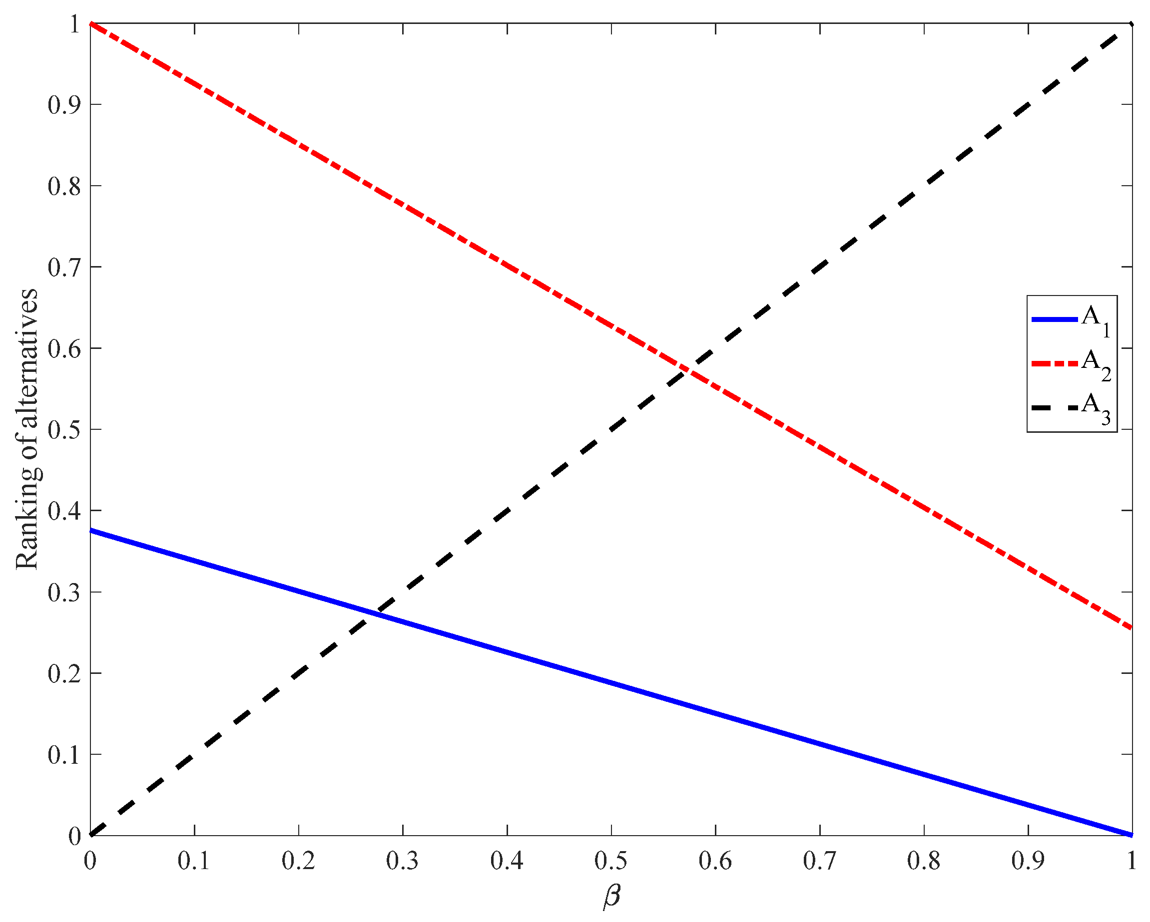
Firstly, the compromise coefficients, $\beta$ and $1-\beta$ in Equation (30) represent the respective weights of $MGU$ and $MGR$. As $\beta$ increases from 0 to 1, the resulting rankings for the three sets of marine equipment ($A_1$, $A_2$, and $A_3$) are depicted in Figure 7.

From Figure 7, it can be observed that the ranking sequence is $A_2>A_1>A_3$ when $\beta$ lies within the range [0, 0.28]; $A_2>A_3>A_1$ when $\beta$ lies within the range [0.28, 0.57]; and $A_3>A_2>A_1$ when $\beta$ lies within the range [0.57, 1]. How can the overall ranking of the three marine equipment sets be defined throughout this process? Following the approach outlined in [11], if the ranking curves for two alternatives ($A_i$ and $A_j$) intersect, both $A_i$ and $A_j$ are classified into the same category. In this context, the three marine equipment sets ($A_1$, $A_2$, and $A_3$) are considered to be tied for first place in the overall ranking.

Second, the proposed method is further examined under a dynamic environment. Specifically, we consider the assessment value $x_{11}^1=\left({\mu }_{11}^1,{\eta }_{11}^1,{\nu }_{11}^1\right)=\left(\mathrm{0.49,0.21,0.18}\right)$ in matrix $M_1$ from Table 5. To simulate variability, we define ${\mu }_{11}^1={\displaystyle \frac{\sigma }{100}}$, ${\eta }_{11}^1=0.7-{\displaystyle \frac{\sigma }{100}}$, where the dynamic parameter $\sigma \in \left[\mathrm{0,69}\right]$. 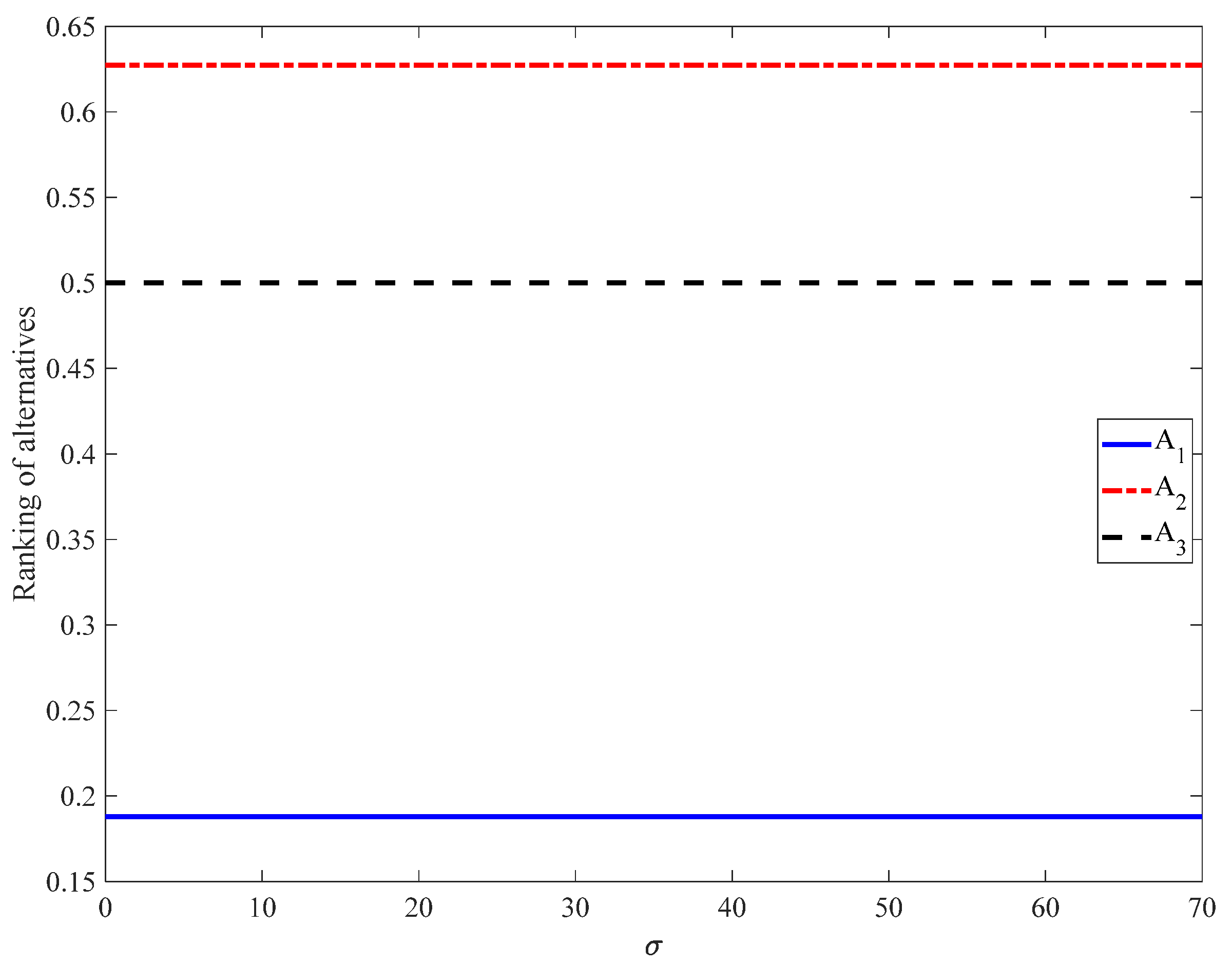All other evaluation values remain consistent with those in Table 5. By setting $\beta =0.5$ in Equation (30) and allowing $\sigma$ to vary from 0 to 69, the dynamic ranking behavior of the three marine equipment alternatives $A_1$, $A_2$, and $A_3$, based on the comprehensive VIKOR index $W_i$, is illustrated in Figure 8.

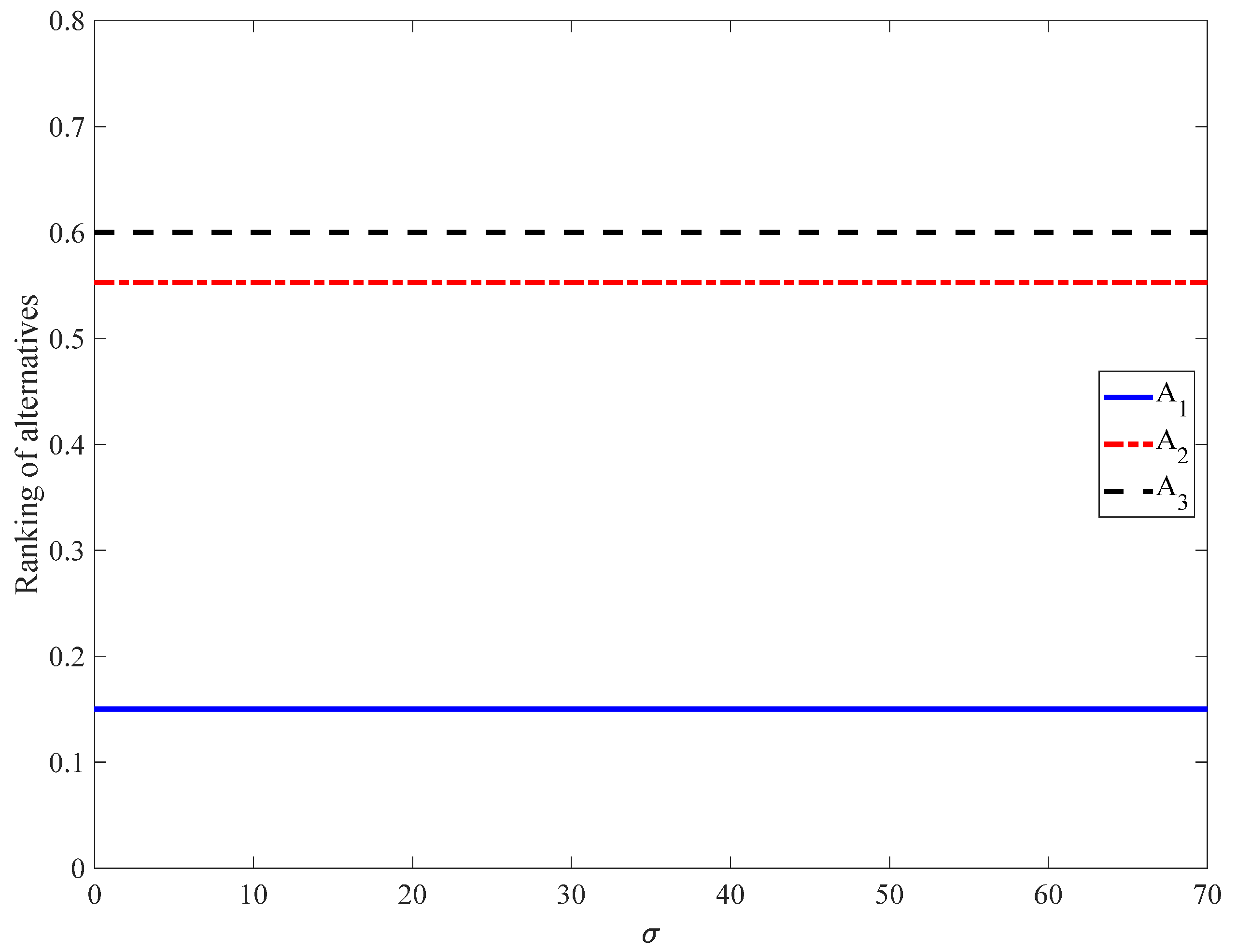
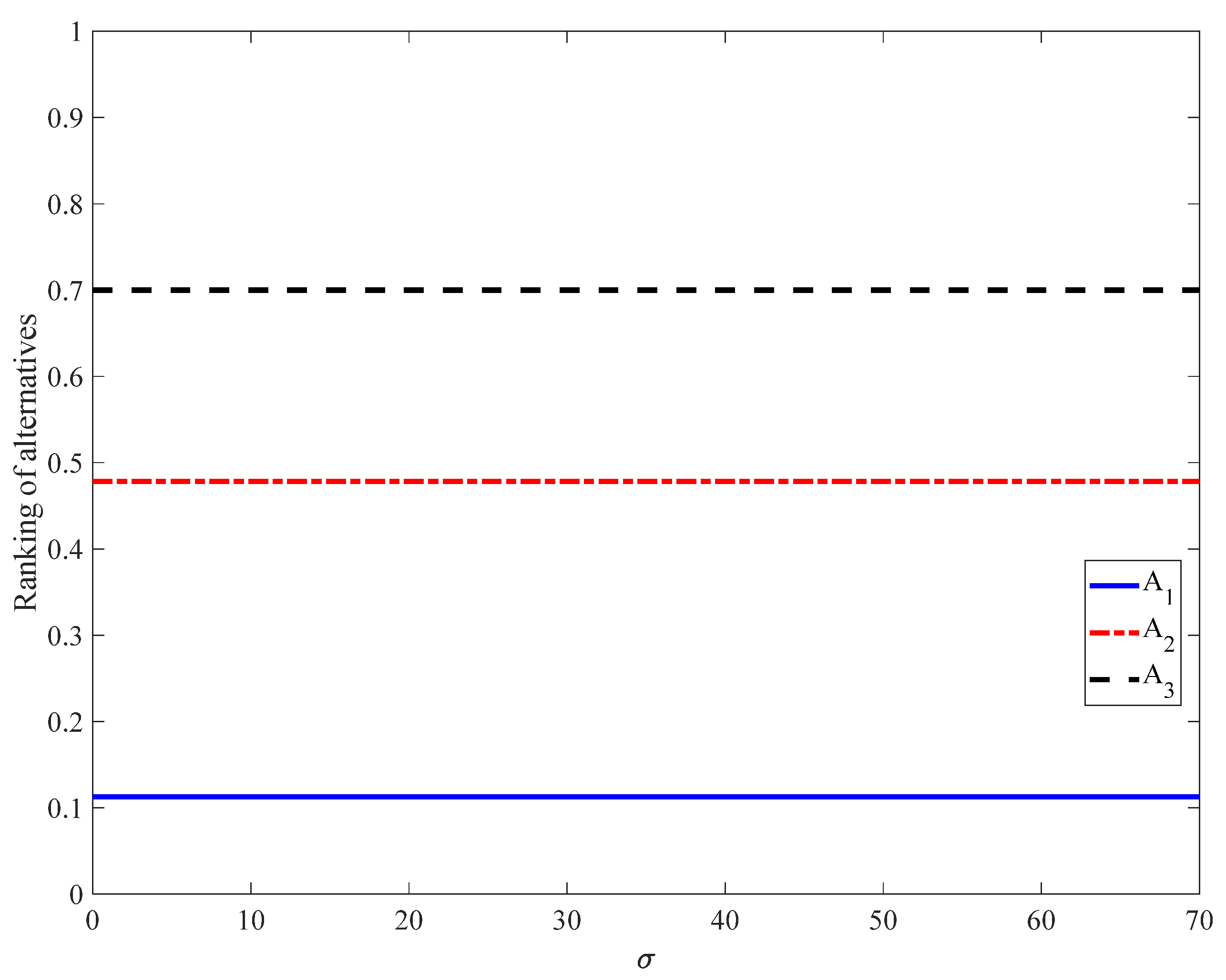
Figure 8 shows that, for $\beta =0.5$, the $W_i\left(\sigma \right)$ values are constant: $A_2=0.6233$, $A_3=0.5$, and $A_1=0.1907$. Thus, the ranking is $A_2>A_3>A_1$. To further investigate the impact of $\beta$, rankings evaluated under the same dynamic conditions for $\beta$ values of 0.2, 0.6, and 0.7 are presented in Figure 9, Figure 10 and Figure 11, respectively.

Figure 9 shows that, for $\beta =0.2$, the $W_i\left(\sigma \right)$ values are constant: $A_2=0.8509$, $A_1=0.3007$, and $A_3=0.2000$. Thus, the ranking is $A_2>A_1>A_3$.

Figure 10 shows that, for $\beta =0.6$, the $W_i\left(\sigma \right)$ values are constant: $A_2=0.6000$, $A_3=0.5528$, and $A_1=0.1503$. Thus, the ranking is $A_3>A_2>A_1$.

Figure 11 shows that, for $\beta =0.7$, the $W_i\left(\sigma \right)$ values are constant: $A_3=0.7000$, $A_2=0.4782$, and $A_1=0.1127$. Thus, the ranking is $A_3>A_2>A_1$. When $\beta$ is set to 1, $W_i$ in Equation (30) reduces to $MG{U}_i$. Conversely, when $\beta$ is set to 0, $W_i$ simplifies to $MG{R}_i$. To further explore dynamic behavior, rankings based on $MG{U}_i$ in Equation (27) under the same dynamic $\sigma$ as Figure 8 and setting $\lambda =0.5$ in Equation (26) are presented in Figure 12.

Figure 12 shows that, for $MG{U}_i$ in Equation (27), the values are constant: $A_3=1.000$, $A_2=0.2546$, and $A_1=0$. Thus, the ranking is $A_3>A_2>A_1$. For the dynamic parameter $\sigma$ as defined in Figure 8 and setting $\chi =0.5$ in Equation (28), rankings based on $MG{R}_i$ in Equation (27) are presented in Figure 13.

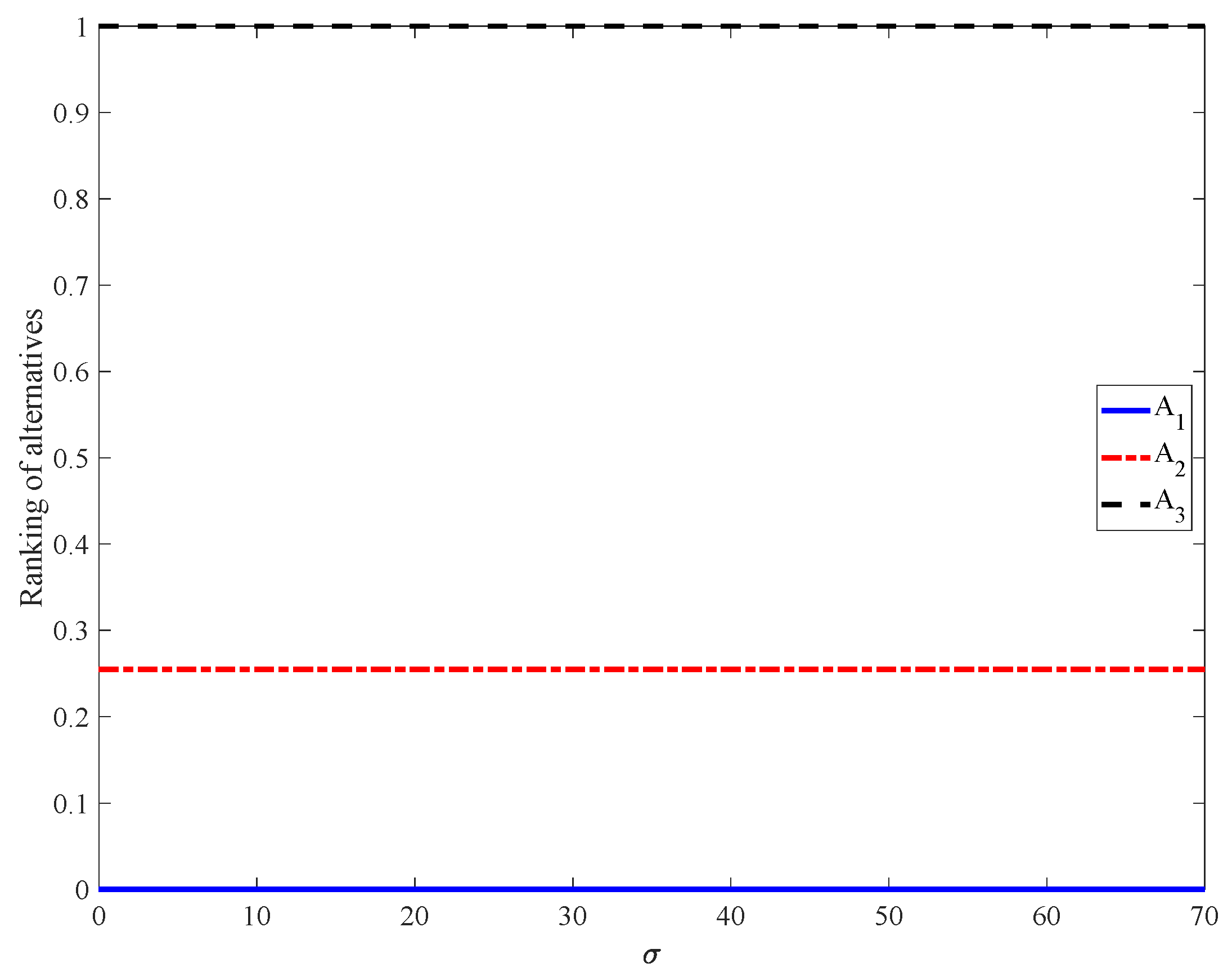
Figure 13 shows that, for $MG{R}_i$ in Equation (29), the values are constant: $A_2=1.000$, $A_1=0.3758$, and $A_3=0$. Thus, the ranking is $A_2>A_1>A_3$. The dynamic changes in ${\mathit{GU}}_i$ were further investigated. Their ranking results were calculated according to Equation (26) and are presented in Figure 14. The experiment used parameter σ as defined in Figure 8 and setting $\lambda =0.5$ in Equation (26).

Figure 14 illustrates that the $G{U}_i\left(\sigma \right)$ curves do not intersect, showing distinct performance levels. Thus, the ranking is $A_3>A_2>A_1$.

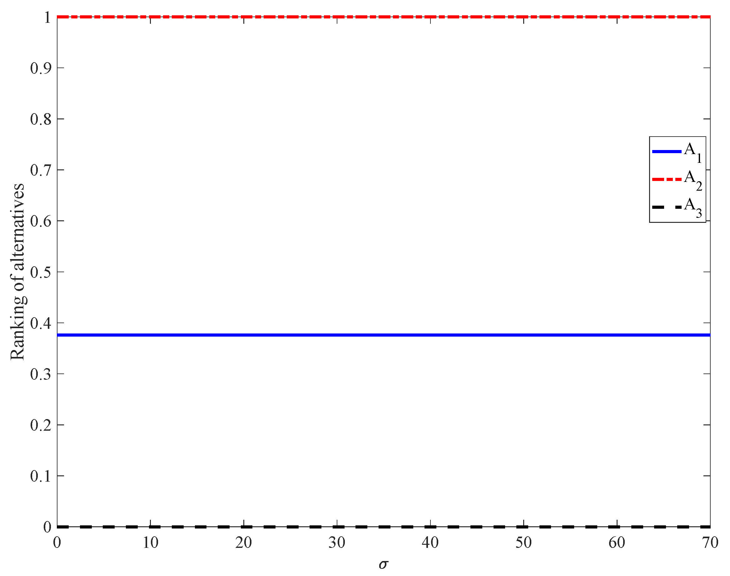
For the VIKOR group regret index $G{R}_i$, a smaller value indicates better performance. To ensure consistency, $G{R}_i$ is transformed as follows:

$$\begin{array}{c}\overline{G{R}_i}=1-{\mathit{GR}}_i,\end{array}$$

(34)

A higher $\overline{G{R}_i}$ corresponds to a superior performance. Figure 15 presents the rankings based on it being transformed, under the same dynamic conditions as depicted in Figure 8.

Figure 15 demonstrates that the three curves do not intersect. Consequently, it can be concluded that the rankings of the three sets of marine equipment are $A_2>A_1>A_3$ based on $\overline{G{R}_i}$ in Equation (34) under this dynamic context.

Based on the above experimental analysis, it is evident that (1) different models may yield varying results, and (2) different experimental conditions may lead to diverse outcomes. A natural conclusion is that the ranking occurring most frequently should be regarded as the most reliable result. The rankings derived from the aforementioned experimental results are presented in

Table 16. Statistics of solutions classified by different experiments.

Measure	${\mathit{A}}_1$	${\mathit{A}}_2$	${\mathit{A}}_3$	$\mathbf{Ranking} \mathbf{with} \mathbf{Classification}$
$MPro{j}_{+}$	✓	✓	✓	$\left\{A_1,A_2,A_3\right\}$
$MPro{j}_{-}$	✓	✓	✓	$\left\{A_1,A_2,A_3\right\}$
$MPro{j}_c$	✓	✓	✓	$\left\{A_1,A_2,A_3\right\}$
$GU$	✓	✓	✓	$\left\{A_1,A_2,A_3\right\}$
$MGU$			✓	$A_3>\left\{A_1,A_2\right\}$
$GR$	✓	✓	✓	$\left\{A_1,A_2,A_3\right\}$
$MGR$		✓		$A_2>\left\{A_1,A_3\right\}$
$W$	✓	✓	✓	$\left\{A_1,A_2,A_3\right\}$
Figure 7	✓	✓	✓	$\left\{A_1,A_2,A_3\right\}$
Figure 8		✓		$A_2>\left\{A_1,A_3\right\}$
Figure 9		✓		$A_2>\left\{A_1,A_3\right\}$
Figure 10			✓	$A_3>\left\{A_1,A_2\right\}$
Figure 11			✓	$A_3>\left\{A_1,A_2\right\}$
Figure 12			✓	$A_3>\left\{A_1,A_2\right\}$
Figure 13		✓		$A_2>\left\{A_1,A_3\right\}$
Figure 14			✓	$A_3>\left\{A_1,A_2\right\}$
Figure 15		✓		$A_2>\left\{A_1,A_3\right\}$
Summary	7	12	12	$\left\{A_2,A_3\right\}>A_1$

.

Table 16 shows that $A_2$ and $A_3$ are the preferred solutions based on the evaluation of all measures.

The experimental results demonstrate that the ranking methods developed in this study for both static and dynamic environments are reasonable. The order relationships of the three sets of marine equipment based on these ranking methods remain stable. These ranking methods constitute a new VIKOR-based group decision-making (GDM) model.

In the long term, investing in reliable equipment is cost-effective, as it reduces the frequency of breakdowns, repairs, and replacements. Companies with a reputation for reliable operations also gain a competitive edge in the maritime industry, attracting clients and ensuring long-term economic viability. To achieve these goals, a scientific and objective evaluation method is crucial. The method proposed in this paper provides powerful support for this purpose: compared to existing methods, its reliability grading of key equipment is clearer, effectively distinguishing between previously indistinguishable equipment grades, and its decision ranking is more stable. This model can accurately identify low-reliability and high-risk equipment, support maintenance prioritization and risk warnings, and help operational departments rationally allocate maintenance resources to improve equipment safety and management efficiency.

8. Conclusions and Further Studies

This paper emphasizes the vital role of reliability assessment in ensuring the environmental and economic sustainability of the shipping industry, addressing the complex challenges that it faces. It presents a novel approach to marine equipment reliability assessment, incorporating symbolic information and a newly developed VIKOR-based pictorial fuzzy projection method. This method introduces four key innovations:

(1)

This paper introduces a novel projection measurement method designed to quantify the proximity between the evaluation and reference matrices within a picture fuzzy environment. Unlike traditional projection methods, this approach overcomes existing limitations and ensures compliance with the normalization condition.

(2)

An average matrix derived from the evaluation matrices provided by the decision-makers (DMs) is adopted as the reference matrix. Building upon this reference, a novel entropy-based approach for determining decision weights is introduced. This method effectively minimizes subjectivity and mitigates the risk of authority monopolization.

(3)

The traditional VIKOR method is extended in this study to establish a novel group decision-making (GDM) framework. In the proposed model, the group utility measure is determined using a combination of the maximum reference matrix, the minimum reference matrix, and the complementary matrix derived from the maximum evaluation matrix. Correspondingly, the group regret measure is formulated based on the minimum reference matrix and the complementary matrix of the maximum evaluation matrix. This approach departs from the classical VIKOR methodology, in which the group regret is calculated solely from the utility matrix. By incorporating multiple reference matrices, the proposed framework substantially enhances the robustness and reliability of decision outcomes.

(4)

A novel ranking method for static environments is introduced, alongside another innovative ranking method tailored for dynamic environments. The practicality and efficacy of these methods are demonstrated through a real-world case study on marine equipment reliability assessment. Furthermore, comparative experimental analyses are performed, benchmarking the proposed methods against existing approaches in the literature.

We acknowledge that, like any model, the proposed approach has its limitations. One key constraint is the reliance on picture fuzzy numbers (PFNs) for representing fuzzy information, which excludes more complex descriptions. While PFNs provide valuable insights, they also have inherent weaknesses. For instance, to the best of our knowledge, there is no well-established subtraction operation for PFNs in the current literature, making it difficult to derive group regret data. Future research could address this limitation by extending the approach to include linguistic fuzzy and hesitant fuzzy environments [81].

Secondly, this study is centered on projection measures and the VIKOR framework for decision-making. Nevertheless, other promising methodologies warrant further exploration, including distance-based evaluation relative to the average solution [82,83], the extended Elimination and Choice Expressing Reality (ELECTRE) approach [84,85], and the Preference Ranking Organization Method for Enrichment Evaluations (PROMETHEE) [62,86,87,88]. These alternatives offer valuable perspectives for future investigations.

Finally, the proposed method has been applied solely to the assessment of marine equipment reliability, with only a single example provided, which is insufficient for comprehensive validation. Future work could explore broader applications of this approach in other relevant domains, such as ship safety assessment or supplier evaluation, to demonstrate its versatility and robustness.