Abstract
It is imperative to comprehend the cyclical variations inherent in liquid methane engines (LMEs) across both design and operational domains. The theoretical thermal efficiency of LMEs is high at higher compression ratios, but the combustion instability also increases. Obtaining relevant metrics from bench experiments is difficult and time-consuming; therefore, in this study, we model tabular data using Conditional GAN (CTGAN) to model the tabular data and generated more virtual samples based on the experimental results of the key metrics (peak pressure, maximum pressure rise rate, and average effective pressure). Through this, a machine learning model was proposed that couples a random forest (RF) model with a Bayesian optimization machine learning model for predicting cyclic variation. The findings indicate that the Bayesian-optimized RF model demonstrates superiority in predicting the metrics with greater accuracy and reliability compared to the gradient boosting (XGBoost) and support vector machine (SVM) models. The R2 value of the former model is consistently greater than 0.75, and the root mean square error (RMSE) is typically lower than 0.3. This paper highlights the promising potential of the Bayesian-optimized RF model in predicting unknown cyclic parameters.
1. Introduction
A significant contributor of global warming is the accumulation of carbon dioxide and other greenhouse gases, the consequences of which are unpredictable but potentially catastrophic [1]. These issues have created considerable challenges and pressures for industries that rely on traditional energy sources, especially the transportation industry. Transport systems are pivotal to the economic development and social progress of any nation [2]. The emergence of new energy vehicles (NEVs) has mitigated this crisis to some extent, but internal combustion engine vehicles still dominate production [3,4,5]. The sustainable development of conventional fuel vehicles is already facing serious challenges. Therefore, the identification of alternative fuels for the transport sector is imperative, given the significant emissions of greenhouse gases (GHGs) and the substantial global demand for oil [6].
On a global scale, a more meaningful and comprehensive response to global warming will require a shift from using fossil fuels to renewable energy sources [7,8]. Natural gas is increasingly recognized as an alternative fuel due to its clean, low-carbon combustion characteristics and its renewability through processes such as biogas and biomethane production [9]. Natural gas has significant advantages over conventional fuels in terms of reduced carbon dioxide emissions and lower pollutant levels [10,11]. Furthermore, natural gas has a wide range of applications, including liquefied natural gas (LNG), compressed natural gas (CNG), and in conjunction with hydrogen as a hydrogen carrier [12]. Compared with CNG, LNG has become the most promising long-distance transportation solution in terms of economic feasibility, environmental sustainability, and technical feasibility [13,14]. LNG engines usually use higher compression ratio (CR) to improve their thermal efficiency. However, the actual design and use of the engine should take into account the engine operating parameters, cycle variations, and other factors. Cycle-to-cycle variations (CCVs) of an engine are fluctuations in engine performance parameters (e.g., power output, combustion efficiency, etc.) from one engine cycle to the next, and these fluctuations affect the average effective torque, overall efficiency, and emissions of the engine [15,16,17]. It is imperative to comprehend and regulate an engine’s CCV in order to enhance its overall efficiency [18].
With the rapid development of data acquisition techniques and computational power, machine learning methods are increasingly being applied in the study of cyclic variations in ignition engines [19]. Among these, cyclic variation prediction has emerged as a new area of research. The experiments and simulations in this study were carried out on a heavy-duty truck engine fueled by liquid methane, and based on this, machine learning techniques (e.g., support vector machines (SVMs), random forest models (RF), and the XGBoost algorithm) were applied to predict cyclic variations and to conduct a comparative analytical study. SVM is an effective regression tool that predicts continuous output values by finding the optimal hyperplane in the data. When dealing with nonlinear problems, SVM can be used with different kernel functions, such as the Gaussian kernel, to deal with complex data relationships. Random forest (RF) is an integrated learning technique that constructs multiple decision trees and aggregates their predictions [20]. This process has been shown to enhance the predictive accuracy and robustness of the model. XGBoost is an efficient gradient-boosting decision tree algorithm that improves on the original gradient-boosting decision tree (GBDT), meaning that the model’s effect is greatly improved. All three methods can effectively handle high-dimensional data and are suitable for applications in the prediction of engine cycle variations, especially when confronted with complex and high-dimensional operating parameters [21,22,23].
Many research teams have incorporated machine learning techniques in the field of internal combustion engine cycle variability. Roy et al. [24] used neural networks to predict the performance and emissions of a variable EGR strategy, high-pressure, common-rail diesel engine, and utilized experimental data to train the neural networks, which enabled the analysis of fuel consumption, effective thermal efficiency, NOx emissions, and other parameters of internal combustion engine cycle variability. Wong et al. [25] used a support vector machine to establish a power and performance model of an internal combustion engine; in their study, the support vector machine could be continuously updated and taught as the training data increased, which was used to continuously improve the accuracy of the support vector machine. Cruz et al. [26] used genetic algorithms to optimize a model of the instantaneous in-cylinder pressure curves of a combustion engine they established, which was more accurate to the dynamic parameters of the internal combustion engine. Through this, they established a more accurate model of the instantaneous in-cylinder pressure of the dynamic process of an internal combustion engine.
Although research teams have conducted a large number of optimization experiments and simulations of internal combustion engines in conjunction with machine learning, most of these efforts have not delved into the prediction of engine cyclic variations. This lack of research is largely due to the complexity and variability of cyclic variations, as well as the difficulty of accurately modeling the complex flow and combustion processes within an internal combustion engine. Although a number of models and techniques have been developed to attempt to predict cyclic variations, these methods often rely on simplifying assumptions or fail to capture all of the factors that affect cyclic variations, limiting the accuracy and reliability of the predictions. Therefore, the development of more accurate prediction tools and methods to improve the accuracy and usefulness of predicting cyclic variations, especially to address the cost required to compute the data and the inaccuracy of the prediction caused by a small amount of data, remains an urgent challenge in the field of internal combustion engine research, which is a problem that this thesis attempts to address. In this experiment, based on the virtual sample generation technique, three improved machine learning models are used to predict the cyclic variation patterns of a liquid methane engine; ultimately, it is shown that the improved models have a better explanation and prediction ability.
2. Experimental Set-Up
2.1. Test Engine and Test Rigs
We modified the technical specifications of the LNG engine to extensively study the characteristics of LME, as shown in Table 1. The measurement of data at varying CR levels was accomplished by utilizing a series of pistons, each characterized by a distinct CR. In order to maintain the contour and dimensions of the piston, only the depth of the deep pit at the top of the piston was machined. This maintained the formation of the vortex at the inlet constant, whilst the CR varied with pit depth [27,28,29]. This allowed the CR to be altered while minimizing the effects of turbulence levels and flame propagation.

Table 1.
Relevant technical parameters of the test engine.
We experimented with a CR value of around 12.6 on the basis of the relationship between the CR and the number of carbon atoms in the molecule [30]. In addition, experiments were conducted with a CR of 16.6, during which the engine produced a discernible knocking and exhibited impaired functionality. A CR of 15.6 can be used as a critical CR. Ultimately, the pistons were manufactured with a CR range of 12.6, 13.6, 14.6, and 15.6.
Various sensors were installed on the LME system according to the relevant requirements. The LME test system comprises multiple modules, the primary of which are the bench control system, the combustion collection and resolution module, the air-intake air-conditioning system, the exhaust gas analysis system, the electric dynamometer, and the data acquisition module, etc. The main equipment and accuracy of the bench test are shown in Table 2, and Figure 1 is a schematic of the LME test.
Table 2.
Part of the test equipment and its related parameters.
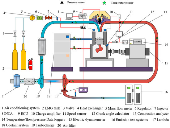
Figure 1.
Schematic layout of the LME test experiment.
Based on the experimental results, the spark timing at various speeds was set to constant values of −14, −20, −22, −24, and −30° CA ATDC at speeds of 800, 1200, 1400, 1600, and 2000 r/min, respectively.
2.2. Experimental Set-Up and Operating Conditions
Bench tests were conducted to investigate the ignition advance angle sweeps and generalized characteristics of the four groups of CRs (12.6, 13.6, 14.6, and 15.6) under typical operating conditions [31]. The locations where boundary conditions were measured in the experiment are shown in Table 3. The main recorded parameters were excess air coefficient (λ), pressure of each major component (intake and exhaust pressure, oil pressure, instantaneous cylinder pressure, cooling water pressure), torque, power, speed, exhaust emissions (HC, COX, NOX), ambient pressure, humidity, and temperature. The general characteristic tests were conducted in accordance with the relevant standards set out by the Chinese government [32].
Table 3.
Boundary conditions for LME benchtop testing.
The test object was the brake mean effective pressure (BMEP), and the conditions were varying from engine idle speed to rated speed, with a speed range of 200 r/min. The load gradually increases from 0 to full load at each speed, with a load range of 2 bar. It was found that the trend of detonation increased as the CR gradually increased. In order to avoid safety accidents and irreversible damage to the engine, the test conditions should be adjusted in real time according to the actual situation [33]. Tests show that the engine’s maximum torque is achieved at 1400 r/min. This paper conducts research on liquid methane engines at this speed. The rotational speed selected for the present study has been determined by our research team to facilitate analysis of the combustion process of LME.
2.3. Uncertainty Analysis
Errors and uncertainties are classified into two categories: fixed and random. Errors can arise from a variety of factors, such as more random environmental conditions, the accuracy and calibration of the instrument, and improper handling by the experimenter [34]. Venu et al. [35] treat uncertainty as ‘accumulated errors’ in the related equipment parameters. This method is also adopted in this study, in that the uncertainty about the outcome is calculated by root mean square (RMS) of errors in a range of relevant test parameters [36]. Equation (1) is its estimation formula.
In above equations, Ur is the uncertainty of the specific parameter at a 5% significance level; and represent the level of measurement and instrumental accuracy, respectively; and the measurement accuracy of some of the experimental equipment is shown in Table 2. Rr and Sr are stochastic uncertainty and systematic uncertainty, respectively, and they are obtained via Equations (2) and (3). Table 4 lists the uncertainties of the various parameters. It is important to note that, since the uncertainty is consistent across all experimental cases, the subsequent transient result plots do not include error bars.
Table 4.
Measured uncertainty (%).
3. Modeling Strategy
3.1. Virtual Data Generation
In machine learning, the generalization ability of a model is a central measure of its efficacy. In practice, virtual sample generation involves the use of prior knowledge of the domain and existing training samples to rationalize the generation of new samples with unknown sample probability distributions. This approach is particularly suitable for domains that require large amounts of data to train complex models, such as deep learning and integration algorithms. Through engine bench tests, we obtained data on the maximum pressure increase rate, and peak pressure with Indicates Mean Effective Pressure (IMEP) at different CRs (11.6, 12.6, 13.6, 14.6, 15.6) and speeds (800 r/min, 1000 r/min, 1200 r/min, 1400 r/min). To ensure data stability, we selected 100 datasets from the entire research. However, the amount of these data is relatively small for building efficient predictive models, and having sufficient training samples is an important basis for improving the generalization ability of traditional supervised learning [37,38]. In order to improve the accuracy and robustness of the model, we can generate more virtual samples based on the actual measurement data of the bench test through a scientifically rational method. Modeling based on small samples is also one of the objectives and significances of this study.
Generative adversarial network (GAN) is a deep learning model that consists of two parts: a generative model and a discriminator model. The generator model is responsible for generating data, and the discriminator model is responsible for evaluating the authenticity of the data. The core function of a GAN is to enable the generator model to produce increasingly realistic data through the adversarial process of the two models. GANs have been widely used in recent years in the fields of data augmentation and rare sample generation [39,40]. However, for tabular data modeling, GANs may cause them to lag behind the baseline in metrics such as the likelihood of synthetically generated data, fitness, and machine learning efficiency [41].
In order to achieve this objective, a further modified GAN model is hereby proposed; namely, the conditional tabular GAN (CTGAN). The model generates data with similar statistical properties by learning the distribution of real data. This is useful for areas such as data privacy, data enhancement, and machine learning applications, and its core function is the same as GAN. Furthermore, the conditional generator of CTGAN facilitates the generation of data that possesses particular discrete values, which can subsequently be employed for the purpose of data augmentation. The working principle of the CTGAN is demonstrated in Figure 2.
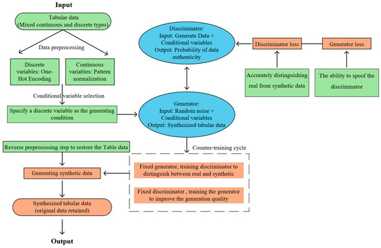
Figure 2.
CTGAN Working Principal Flowchart.
3.2. Data Classification and Normalization
The majority of machine learning models necessitate the preliminary processing of input data, eschewing the utilization of raw data. The output of the model will be dominated by an input parameter that is significantly larger than the range of the other parameters. It is imperative that the initial inputs are normalized in order to eliminate the detrimental effect. The problem of the effect of dimensionality in this study was addressed using a center normalization approach, which is based on the principle of Equation (4), where x is the original data value, is the mean of the data, and is the standard deviation of the data.
The construction of a predictive model necessitates the meticulous division of the dataset. In this study, the K-fold cross-validation method was employed to divide the data. The method classifies the original dataset into K random folds, of which K-1 folds are used for model training and the remaining folds are designated as test data. The opportunity is provided for each sample to train and test the model, which ensures the generalizability of the model and avoids unreliable results being obtained from fixed proportions of the dataset. An elevated K engenders elevated computational expense and complexity, whilst a diminished K precludes the capacity to formulate adequate predictions; the K used in this model is 5.
The performance of the various models is to be assessed. To this end, two commonly utilized metrics, coefficient of determination (R2) and root mean square error (RMSE), are employed. R2 indicates the proportion of the variation in the dependent variable that can be explained by the independent variable, and it is a measure of the fit of the regression model. It can thus be used to measure how well the model fits the observed data. RMSE is a measure of the predictive accuracy of a model, which is used to assess the difference between the predicted value and the true value.
3.3. Machine Learning Prediction
SVM is a machine learning method based on structural risk minimization and statistical learning theory. The algorithm employs a kernel technique to project data into a high-dimensional space for linear analysis. SVM aims to find the best balance between the model complexity and learning performance to optimize the model’s ability to generalize, i.e., to efficiently identify new samples while maintaining a high level of accuracy on the training samples. This property means that SVM performs particularly well in dealing with nonlinear problems on small datasets [42]. The kernel function K is mainly used to simplify the operation in high-latitude space, and the process is shown in Equation (5).
The above equation is the penalty factor and i is the slack variable. In this study, a Gaussian kernel function is used, so the parameter penalty coefficient needs to be determined, which controls the complexity of the model; the larger its value, the greater the penalty for misclassification and the higher the complexity of the model [43]. From the SVM parameter optimization results, the penalty function value is 0.1758, the kernel function parameter is 6.1315, and the settings of the three parameters are shown in Table 5. The research process is shown in Figure 3.
Table 5.
SVM Important Parameter Settings.
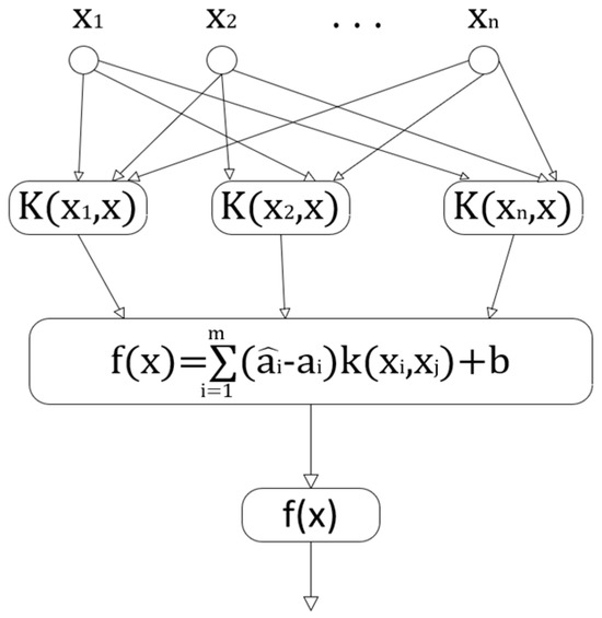
Figure 3.
Schematic of SVM.
Random forest (RF) is an integrated algorithm that is generally better than a single decision tree. A decision tree implements regression by keeping the MSE as low as possible, and the decision tree makes judgements in each branch and decides on the best outcome. Random forests integrate multiple decision trees and introduce randomness in the extraction of samples and features to obtain the optimal solution by ‘voting’ among multiple decision trees [44]. The RF process is shown in Figure 4.
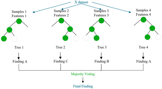
Figure 4.
Schematic of RF.
The importance score obtained by the RF in the decision-making process is usually measured by the Gini index G. is the Gini index of node t in the decision tree, and its expression is shown in Equation (6); k denotes the kth category in the node, and n is the number of categories contained in node t. The importance of variable x at node t, i.e., the amount of change in the Gini index before and after branching of node t, is expressed as Equation (7), where and are the Gini indices of the two nodes after branching.
If the set of all nodes of variable in decision tree i is , then the importance score of in the ith tree is shown in Equation (8). Finally, the importance score of variable x is obtained by averaging the scores of each decision tree, which is then further normalized.
The number of base learners is one of the main factors determining the accuracy of the RF. The performance of the algorithm in relation to the number of base learners should first be analyzed before it is first used. We chose 800 peak pressures for each of the different CRs (12.6, 13.6, 14.6, 15.6) as the overall sample, the number of cycles as the input sample, and the peak pressure as the output sample, of which 70% was used as the training set and 30% as the test set. The other hyperparameters were taken as default values, and only the number of base learners is changed for training. As demonstrated in Figure 5, the RMSE of the model is influenced by the quantity of the model’s learning devices. It is evident that as the quantity of learning devices increases, the RMSE and the R2 of the training and test sets remain stable. However, there is a significant discrepancy between the training and test sets, indicating a relatively severe over-simulation phenomenon in the model. This suggests that there is considerable potential for improvement in the algorithm.
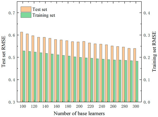
Figure 5.
Variation in RMSE for different numbers of base learners.
In the realm of contemporary parameter optimization, the utilization of Bayesian optimization has emerged as a pioneering approach. The main optimization process of this method is to find an acceptable maximum value by guessing the black box function when the black box function is unknown. The optimization process is bifurcated into two fundamental stages: the prior function (PF) and the acquisition function (AC) [45]. The subsequent algorithm process is outlined as follows: Firstly, the known data is analyzed to determine the hyperparameters to be tuned, which include the base learner, maximum depth, maximum number of features used in a single decision tree, and node splitting value. Secondly, the hyperparameters are optimally tuned based on Bayesian optimization [46]. The code for this is displayed in Table 6. Bayesian optimization was used to find the optimal hyperparameters in different models. Utilizing the RMSE of the test set in the 5-fold cross-validation as the optimization index, the number of optimization iterations is set to 300, resulting in the optimal parameter combination as illustrated in Table 7.
Table 6.
Bayesian optimization pseudo-code.
Table 7.
Interpolation rate classification table.
XGBoost is a highly effective gradient-boosting decision tree algorithm. It was developed by enhancing the gradient-boosting decision tree (GBDT) algorithm, thereby significantly enhancing its efficacy. As a forward-looking model, its fundamental principle is to employ a combination of ideas from the “boosting” theory to integrate multiple weak learning devices into a single strong learning device. That is to say it utilizes the collective decision-making of multiple trees, with the resulting value being the difference between the target value and the forecasts of all previous trees. The sum of all results is then added to obtain the final result, thereby enhancing the effectiveness of the entire model. The objective function is shown in Equation (9).
where is the loss function revealing the training error, and is the regularization definition complexity. The XGBoost modeling process is shown in Figure 6.
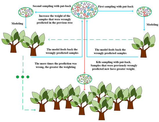
Figure 6.
XGBoost Gradient-Boosting Tree Modeling Process.
As illustrated in Figure 7, with the augmentation of the number of base learners, the overall RMSE of the test set exhibits an upward trend, accompanied by greater fluctuations, suggesting that the XGBoost model demonstrates a lower level of stability compared to the RF model; however, it exhibits a higher degree of overfitting. The existence of a more extensive optimization space, similar to the aforementioned Bayesian model optimization approach, is revealed.
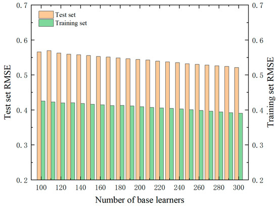
Figure 7.
Variation in RMSE for different numbers of base learners.
In a similar manner, the hyperparameters that require tuning are determined as follows: base learner, maximum depth, learning rate, and proportion of samples taken by random sampling. Subsequently, the hyperparameters undergo optimization for tuning based on Bayesian optimization. The RMSE of the test set in the 5-fold cross-validation is utilized as the optimization index. The number of optimization iterations is set to 300, which results in the optimal parameter combinations, as shown in Table 8.
Table 8.
Interpolation rate classification table.
This study was conducted based on little virtual data generated from a small sample. For situations with smaller data volumes, supervised learning methods such as SVM, RF, and XGBoost are more effective [47]. For cases with obvious threshold effects (such as engine knocking), the decision boundary characteristics of SVM can accurately capture this nonlinear transition [48].The RF model randomly selects features to reduce interference from irrelevant features [49]. In addition, as a benchmark model, RF can quickly verify data quality. XGBoost can auto-handle missing values and feature scaling, and make the most of limited real data [50].
4. Results and Discussion
4.1. LME Cycle Variability Study
In the experimental phase of the study, the in-cylinder pressure variation with crank angle (CA) was measured for 100 cycles at CRs of 13.6, 14.6, and 15.6. The results of this experiment are illustrated in Figure 8. BMEP is the brake mean effective pressure.
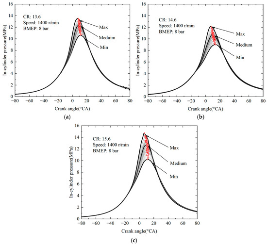
Figure 8.
Effect of compression ratio on cyclic variation in in-cylinder pressure. (a) CR = 13.6 (b) CR = 14.6 (c) CR =15.6.
As the compression ratio increases, the peak pressure tends to increase. As demonstrated in Figure 8a, at a compression ratio of 13.6, the peak pressure is reduced. This indicates that the mixture exhibits a lower pressure and temperature at ignition, which may consequently yield suboptimal combustion efficiency. As demonstrated in Figure 8b, an increase in the compression ratio to 14.6 results in a more compacted mixture at the point of ignition. This, in turn, leads to higher pressures and temperatures, thereby enhancing combustion efficiency and generating greater engine output. As demonstrated in Figure 8c, an augmentation in compression ratio to 15.6 results in a discernible escalation in peak pressure. In such conditions, it can be deduced that the thermal efficiency of the engine is likely to be the highest among the three.
Cyclic variation in in-cylinder pressure is defined as the difference between the maximum and minimum values of in-cylinder pressure that are attained by the engine across multiple cycles. When the compression ratio is 13.6, the peak pressure curve appears to be relatively concentrated, indicating that the cyclic variation in cylinder pressure is relatively small at this point. This observation is consistent with the hypothesis that stable engine operation is indicative of a relatively consistent combustion process from cycle to cycle. As the compression ratio increases, the range of cyclic variations concomitantly increases. A wider range of variations is exhibited at a compression ratio of 14.6 than at a compression ratio of 13.6. It is evident that at a compression ratio of 15.6, the discrepancy between the maximum and minimum pressures and the mean in-cylinder pressure curve is the most pronounced. This observation signifies that the uniformity of the combustion process exhibits a decline across varying cycles. Consequently, the stability of engine operation is diminished, and the combustion efficiency and engine performance undergo substantial fluctuations. This, in turn, leads to an augmented risk of engine blowout.
Notwithstanding the numerous advantages of an increased compression ratio, the process can result in premature spontaneous combustion of the mixture. This, in turn, creates a pressure wave within the engine, which can lead to damage and a consequent reduction in the engine’s performance and longevity [33]. As illustrated in Figure 9, the peak pressures were measured for 100 cycles, with CRs of 12.6, 13.6, 14.6, and 15.6 at speeds of 1400 r/min for 8 bar, 10 bar, and 12 bar, respectively.
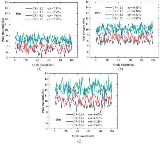
Figure 9.
Effect of Compression Ratio on Peak Pressure Cycle Variation. (a) 8 bar (b) 10 bar (c) 12 bar.
The prevailing tendency for the peak pressure to increase as the compression ratio increases is attributed to the fact that a higher compression ratio results in the release of a greater quantity of energy from the combustion process. As the engine load increases, the average peak pressure value gradually increases at the same compression ratio. As the compression ratio increased from 8 bar, the cyclic variations in the four different ratios became more apparent, with the coefficient of variation (COV) values recorded as 7.5%, 7.5%, 7.0%, and 7.1%, respectively. This finding indicates that increase in compression ratio exerts minimal influence on the stability of peak pressures under low-load conditions. At 10 bar, the peak pressure COV values demonstrate a decreasing trend as the compression ratio increases, initially decreasing from 6.3% to 5.5%, and then increasing slightly to 5.8%. This indicates that the stability of peak pressure increases and then decreases as the compression ratio increases at moderate loads. The maximum COV value of 7.7% was obtained at 12 bar with a compression ratio of 15.6, while the minimum COV value of 5.8 % was achieved at a compression ratio of 14.6. It has been established that, at a constant engine load, an increase in the compression ratio results in an increase in the average peak pressure. For a constant CR, an increase in engine load is associated with an upward trend in mean peak pressure. With regard to the prevailing tendency, an augmentation in compression ratio may result in a decline, followed by an increase, in peak pressure volatility. This phenomenon occurs due to the fact that, within a specific range, the combustion of the mixture becomes more stable as the compression ratio increases. This, in turn, helps to reduce pressure fluctuations between cycles.
The maximum pressure rise rate is defined as the maximum rate of pressure increase during a given cycle. This rate has proven to profoundly affect the combustion performance and overall efficiency of the engine [51]. Increased CRs are associated with elevated temperatures and pressures of the fuel and air mixture at the termination of the compression stroke. The presence of high temperatures and pressures in this environment has been demonstrated to increase the ignition and combustion rates of the fuel. The acceleration of fuel combustion leads to a rapid increase in pressure over a brief period, thereby enhancing the thermal efficiency and power output of the engine. While a rapid increase in pressure can offer certain advantages, it concomitantly engenders a heightened risk of engine blowout. Premature spontaneous combustion of the fuel and air mixture may result in an uncontrolled combustion process in engines with relatively high compression, leading to the formation of a high-amplitude pressure wave. This process is known as engine knock.
The phenomenon of engine knock, also known as “bursting”, has been shown to have a number of deleterious effects on the performance of the engine [52]. Firstly, it has been demonstrated that this phenomenon can lead to a reduction in the operational efficiency of the engine. Secondly, it has been demonstrated that engine knock can cause damage to key components, such as pistons, cylinders, and spark plugs. This, in turn, can have a detrimental effect on the economy, durability, and reliability of the engine.
As illustrated in Figure 10, the maximum pressure rise rate exhibits a cyclical variation at CRs of 12.6, 13.6, 14.6, and 15.6 at a speed of 1400 r/min and a load of 12 bar. The maximum observed pressure rise rate was 0.184 MPa/°CA at a CR of 12.6. It was observed that, under these conditions, the fluctuation in the pressure rise rate exhibited enhanced stability, and the combustion process demonstrated increased homogeneity.
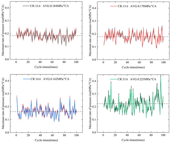
Figure 10.
Cyclic variation in CR against maximum rate of pressure rise.
The mean maximum pressure rise rate is marginally lower at 0.178 MPa/°C and has a CR of 13.6. The expected rate of pressure rise is generally known to increase with the CR. However, in this particular instance, a decline in pressure rise is observed. This phenomenon is most likely attributable to the necessity for the combustion management system (for example, ECU calibration) to take into consideration the impact of emissions at higher CRs. At a CR of 14.6, the average maximum pressure rise rate is reduced further to 0.162 MPa/°CA. This finding indicates that the combustion process is more favorable at this CR, suggesting that the EMS (engine management system) may be regulating the combustion rate with great efficacy. It was found that the mean maximum pressure rise rate increased to a maximum of 0.223 MPa/°C at a CR of 15.6, which was the highest of the four CRs. The higher rise rate causes combustion to occur more rapidly and violently within the engine, generating abnormal pressure waves and substantially increasing the risk of triggering an engine blowout.
4.2. Analysis of CTGAN Data Generation Results
The generation of 400, 700, and 1000 virtual dataset was achieved by employing the CTGAN method, utilizing peak pressures from 100 bench tests conducted at a speed of 1400 r/min and under an operating condition of 8 bar, with CRs of 12.6, 13.6, 14.6, and 15.6.A box-and-line diagrams of the experimental and virtually generated data shown in Figure 11. A comparison of the primary parameters presented in the figure can be found in Table 9.
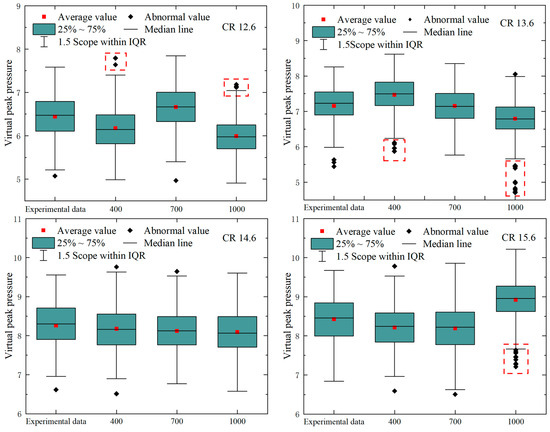
Figure 11.
The box-and-line diagram of virtually generated data with different CR.
Table 9.
Main Parameters of box-and-line diagram.
In the event of the data being normally distributed, the Standard Deviation (Std) is approximately equal to the interquartile range (IQR) divided by 1.35. However, the Std of the 1000 virtual data is significantly larger than the IQR divided by 1.35, which indicates that the data may contain skewed or extreme values. Furthermore, the Std of the other two groups of virtual data is slightly smaller than the IQR divided by 1.35, which is similar to the experimental data. When considered in conjunction with Figure 11, it becomes evident that the data generated by 1000 instances of virtualization exhibit the highest number of anomalies. The distribution exhibits a tendency to the lower end, indicating instability in the data and the potential for underfitting or overfitting phenomena.
The 700 virtualizations exhibited a reduced incidence of anomalies in comparison to the 400 virtualizations, and the scores demonstrated increased symmetry and stability. The mean trend line graph with residual scatter plot of the generated data is demonstrated in Figure 12.
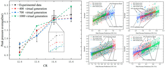
Figure 12.
Mean Trend Line Plot and Residual Scatter Plot for Virtual Data.
A consideration of both the mean trend line graph and the residual scatter plot reveals that the data of 1000 virtual cycles exceeded the range of the mean error bars of the original data on two occasions. Furthermore, the distribution was found to be non-random at a CR of 13.6. This suggests that the model may be biased. Although the data from 400 virtual cycles falls within the error bars, the residual scatter plot exhibits a greater number of outliers than 700 virtual cycles, thereby compromising the robustness of the model. The mean error values for the 700 virtual cycles demonstrate a high degree of similarity with regard to trends when juxtaposed with the mean error values for the original dataset. Moreover, the residual values appear to be randomly distributed around the zero-line, thus indicating the absence of any discernible pattern in their distribution. It is also noteworthy that no outliers are observed, with no substantial residuals recorded. This result indicates that the model with 700 virtual cycles may not have significant errors. Additionally, there is an absence of discernible heteroscedasticity, with the scatter of residuals exhibiting comparable degrees of variability across various levels of predicted values.
Wasserstein Distance is a measure of the difference between two statistical distributions. In recent years, Wasserstein Distance has become increasingly popular in machine learning and data science due to its stable and geometric intuition [53]. Compared with KL divergence and JS divergence, Wasserstein distance can still reflect the distance between two distributions even if they do not overlap [54]. To quantify the quality of virtual data, we calculated the Wasserstein distance between 400, 700, and 1000 virtual generations compared to real data at different CRs. The results are shown in Figure 13.
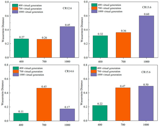
Figure 13.
Wasserstein distance between virtual data and original data at different CRs.
According to Figure 13, at lower CRs (12.6 and 13.6), the 400 and 700 virtual generations are significantly better than the 1000 virtual generation. At a CR of 14.6, 700 virtual generation are weaker than 400 and 1000 virtual generations. At a CR of 15.6, the Wasserstein Distance of 700 virtual generation and 1000 virtual generation is nearly the same, but both are weaker than 400 virtual generation.
To summarize, it is evident that upon reaching 700 virtual generated cycles, the model is capable of capturing the distributional characteristics and tendencies of the data with greater precision. This enhances the balance and comprehensiveness of the data representation, thus avoiding the dangers of overfitting or underfitting. Consequently, this enhancement results in an enhancement in the model’s prediction performance. The final 800 peak pressures (with 700 virtual data) at different CRs (12.6, 13.6, 14.6, 15.6) are shown in Figure 14. Utilizing these as raw data to train the model enhances the model’s generalization capability.
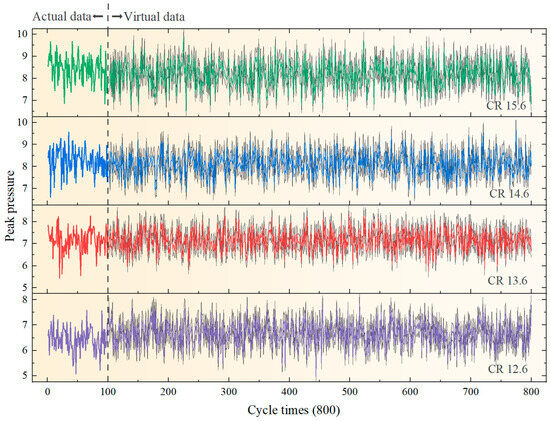
Figure 14.
Virtual stress training data.
4.3. Cyclic Variation Prediction Based on Machine Learning
The following section will present an example of analysis of SVM-based cyclic variation in important parameters. The selection process involved the allocation of 70% of the samples as the training set and the remaining 30% as the validation set. The parameter kernel function employed is of the Gaussian type. The important parameter settings in the SVM model are shown in Table 5. As illustrated in Figure 15, the peak pressure prediction plots for the training and test sets are shown. Despite the identification of the optimal penalty and kernel function parameters, the SVM model remains variable and fails to accurately track the fluctuations and trends of the data.
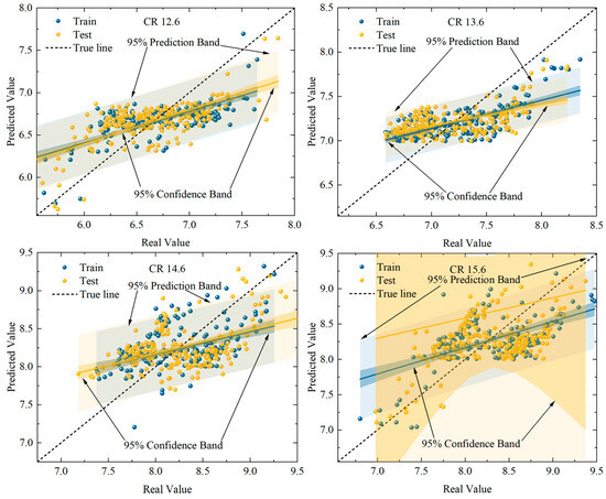
Figure 15.
Comparison of peak pressure prediction performance of SVM models.
The results of the metrics for the training set at varying CRs were obtained by training the other observables (pressure elevation rate, IMEP), as illustrated in Table 10. This model demonstrates limited generalization capability for peak pressure and is unable to adapt to data with complex distributions.
Table 10.
Comparison of the prediction accuracy of SVM model across observations.
The optimal parameters obtained from Table 7 are substituted into the model to establish the optimal RF model, and are substituted into the data for modeling and analysis as follows: the training set and test set of the model can be more evenly distributed on both sides of the true line. As demonstrated in Figure 16, the model demonstrates a high degree of fit. A comparison of the default parameter model and the improved model with Bayesian optimization reveals that the improved model exhibits a reduced overall overfitting degree, a reduced RMSE for the test set, and an increased R2. This indicates that the performance of the improved model has been enhanced to a certain extent.
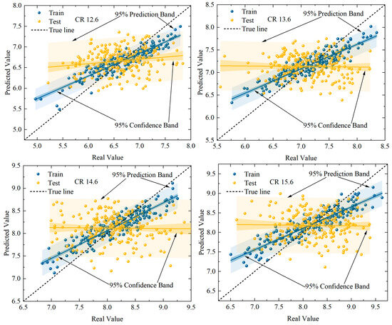
Figure 16.
Comparison of peak pressure prediction performance of RF models.
The results of the metrics for its training set at varying CRs were obtained by training the other observables (pressure rise rate, IMEP), as illustrated in Table 11. It has been observed that different CRs do not have a significant effect on the prediction of cyclic variations, especially with regard to the accuracy of prediction of peak pressure and IMEP. The data indicates that the four CRs (12.6, 13.6, 14.6, and 15.6) demonstrate superior performance in the majority of cases, exhibiting higher explanatory power and enhanced accuracy in prediction. The enhanced complexity of the combustion process at elevated CRs did not exert a substantial negative influence on the predictive performance of the RF model. The prediction results of the RF model have been shown to be both stable and accurate, and robust to outliers.
Table 11.
Comparison of the prediction accuracy of RF model across observations.
The optimal combination of hyperparameters, as determined by Table 8, is then incorporated into the model to construct the most effective XGBoost model, which is subsequently applied to the initially segmented test set. As demonstrated in Figure 17, the XGBoost model demonstrates enhanced stability and predictability in comparison to the SVM; however, it does not reach the level of efficacy exhibited by the Bayesian-optimized RF model.
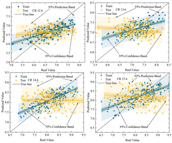
Figure 17.
Comparison of peak pressure prediction performance of XGBoost models.
The results of the metrics for the training set at varying CRs were obtained by training the other observables (pressure rise rate, IMEP), as illustrated in Table 12. As demonstrated by the data, lower compression ratios (12.6 and 13.6) have been shown to yield superior outcomes in the majority of cases, exhibiting higher explanatory power and enhanced accuracy in prediction. It has been observed that an increase in CR has a detrimental effect on the predictive performance of the model. The RMSE values of all three metrics at higher CRs (14.6 and 15.6) have been determined to exceed those at lower CRs. This phenomenon may be attributed to the augmentation in complexity of the combustion process at higher CRs.
Table 12.
Comparison of the prediction accuracy of XGBoost model across observations.
As illustrated in Figure 18, the R2 values for the various model training sets are compiled to provide a comprehensive overview of the predictive performance of the models. With regard to R2, the following models were found to be most effective: RF > XGBoost > SVM. This finding indicates that the RF model provides the optimal fit. Furthermore, the prediction accuracy and robustness of the three observables in the RF model are thoroughly validated, as shown in Figure 19. The cycle-to-cycle variations for different models at different CRs are shown in Table 13.
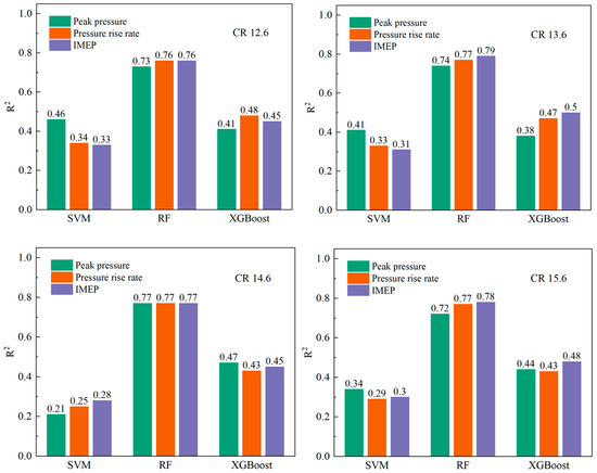
Figure 18.
R2 results for the training set of different models at four CR.
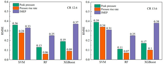
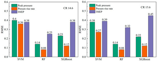
Figure 19.
Training set RMSE results for the three observables for different models.
Table 13.
Cycle-to-cycle variations in different models at different compression ratios.
5. Conclusions
Limited by time, research content, and length, we have not yet conducted research on other input parameters. In addition, it is meaningful to extend this study to hydrogen-enriched methane or other biofuels. Whether the model output results can be mapped back to engine physical parameters (such as knock risk zone and optimal compression ratio) is also an area that we need to further explore. The analysis of cyclic variations facilitates the identification of instabilities in the engine’s operational dynamics. The present study investigates the combustion of a high-compression-ratio liquid methane engine, drawing on a combination of experimental and modeling simulations. In addition, machine learning algorithms are employed to predict cycle variations. The principal contributions of this study are summarized as follows:
- (1)
- The present study investigates the effect of compression ratio on cycle variations and their key indexes. This is achieved by means of cycle–cycle statistics and analysis of cylinder pressure test data. The results demonstrate that as the compression ratio increases, the consistency of the combustion process in different cycles decreases, and the stability of engine operation decreases. Concurrently, the enhancement in compression ratio instigates an oscillatory pattern in peak pressure, characterized by an initial decrease and subsequent increase. The increase in compression ratio also leads to an increase in the average maximum pressure rise rate. However, when the compression ratio is elevated from 12.6 to 13.6, a decline in the pressure rise rate is observed. This phenomenon can be attributed to the enhanced efficacy of the combustion management system at higher compression ratios, as evidenced by the modulation of ignition timing and fuel injection strategy.
- (2)
- Machine learning algorithms were employed in conjunction with enhanced SVM, RF, and XGBoost models to predict and compare cyclical variations in peak pressure, maximum pressure rise rates, and IMEP. The results demonstrate that the RF model, following Bayesian optimization, exhibits the most optimal prediction efficacy, with an R2 value that consistently exceeds 0.7 and minimal RMSE values consistently less than 0.3. This study underscores the efficacy of RF models in accurately predicting cyclic variations in liquid methane engines. Bayesian optimization algorithms have the capacity to enhance the predictive performance of the model by facilitating the selection of hyperparameters, and the model in question has been demonstrated to exhibit favorable indicators with regard to the prediction of peak pressure, maximum pressure rise rate, and IMEP. When making predictions, peak pressure is affected by fluctuations, causing data concentration and resulting in a large CCV. In combustion control, IMEP is the result of response performance. IMEP predictions are easier to make. Therefore, IMEP predictions are more accurate than peak pressure predictions.
Author Contributions
Conceptualization, E.Z. and F.Z.; Methodology, J.L.; Software, E.Z.; Validation, E.Z.; Formal analysis, X.D.; Investigation, E.Z.; Writing—original draft, E.Z.; Writing—review & editing, F.Z. and H.X.; Project administration, F.Z.; Funding acquisition, F.Z. All authors have read and agreed to the published version of the manuscript.
Funding
This research work is sponsored by the Hunan Provincial Natural Science Foundation of China (2023JJ41056) and Hunan Provincial Department of Education Project of China (24A0202).
Data Availability Statement
The data presented in this study are available on request from the corresponding author. The data are not publicly available due to future work.
Acknowledgments
The authors appreciate the reviewers and the editor for their careful reading and many constructive comments and suggestions on improving the manuscript.
Conflicts of Interest
The authors declare no conflict of interest.
References
- Omer, A.M. Energy, environment and sustainable development. Renew. Sustain. Energy Rev. 2008, 12, 2265–2300. [Google Scholar] [CrossRef]
- Othman, M.F.; Adam, A.; Najafi, G.; Mamat, R. Green fuel as alternative fuel for diesel engine: A review. Renew. Sustain. Energy Rev. 2017, 80, 694–709. [Google Scholar] [CrossRef]
- Alkhathlan, K.; Javid, M. Carbon emissions and oil consumption in Saudi Arabia. Renew. Sustain. Energy Rev. 2015, 48, 105–111. [Google Scholar] [CrossRef]
- Elgohary, M.M.; Seddiek, I.S.; Salem, A.M. Overview of alternative fuels with emphasis on the potential of liquefied natural gas as future marine fuel. Proc. Inst. Mech. Eng. Part M J. Eng. Marit. Environ. 2014, 229, 365–375. [Google Scholar] [CrossRef]
- Ramey, V.A.; Vine, D.J. Oil, Automobiles, and the U.S. Economy: How Much Have Things Really Changed? NBER Macroecon. Annu. 2011, 25, 333–368. [Google Scholar] [CrossRef]
- Surawski, N.C.; Ristovski, Z.D.; Brown, R.J.; Situ, R. Gaseous and particle emissions from an ethanol fumigated compression ignition engine. Energy Convers. Manag. 2012, 54, 145–151. [Google Scholar] [CrossRef]
- Rabbi, M.F.; Popp, J.; Máté, D.; Kovács, S. Energy Security and Energy Transition to Achieve Carbon Neutrality. Energies 2022, 15, 8126. [Google Scholar] [CrossRef]
- Zhou, F.; Wu, C.; Fu, J.; Liu, J.; Duan, X.; Sun, Z. Abnormal combustion and NOx emissions control strategies of hydrogen internal combustion engine. Renew. Sustain. Energy Rev. 2025, 219, 115847. [Google Scholar] [CrossRef]
- Wan, S.; Zhou, F.; Fu, J.; Yu, J.; Liu, J.; Abdellatief, T.M.M.; Duan, X. Effects of hydrogen addition and exhaust gas recirculation on thermodynamics and emissions of ultra-high compression ratio spark ignition engine fueled with liquid methane. Energy 2024, 306, 132451. [Google Scholar] [CrossRef]
- Paul, A.; Bose, P.K.; Panua, R.S.; Banerjee, R. An experimental investigation of performance-emission trade off of a CI engine fueled by diesel–compressed natural gas (CNG) combination and diesel–ethanol blends with CNG enrichment. Energy 2013, 55, 787–802. [Google Scholar] [CrossRef]
- Wei, H.; Zhang, R.; Chen, L.; Pan, J.; Wang, X. Effects of high ignition energy on lean combustion characteristics of natural gas using an optical engine with a high compression ratio. Energy 2021, 223, 120053. [Google Scholar] [CrossRef]
- El-Gohary, M.M. The future of natural gas as a fuel in marine gas turbine for LNG carriers. Proc. Inst. Mech. Eng. Part M J. Eng. Marit. Environ. 2012, 226, 371–377. [Google Scholar] [CrossRef]
- Arteconi, A.; Brandoni, C.; Evangelista, D.; Polonara, F. Life-cycle greenhouse gas analysis of LNG as a heavy vehicle fuel in Europe. Appl. Energy 2010, 87, 2005–2013. [Google Scholar] [CrossRef]
- Kumar, S.; Kwon, H.-T.; Choi, K.-H.; Lim, W.; Cho, J.H.; Tak, K.; Moon, I. LNG: An eco-friendly cryogenic fuel for sustainable development. Appl. Energy 2011, 88, 4264–4273. [Google Scholar] [CrossRef]
- Kyrtatos, P.; Brückner, C.; Boulouchos, K. Cycle-to-cycle variations in diesel engines. Appl. Energy 2016, 171, 120–132. [Google Scholar] [CrossRef]
- Reyes, M.; Tinaut, F.V.; Giménez, B.; Pérez, A. Characterization of cycle-to-cycle variations in a natural gas spark ignition engine. Fuel 2015, 140, 752–761. [Google Scholar] [CrossRef]
- Yang, Z.; Steffen, T.; Stobart, R. Disturbance Sources in the Diesel Engine Combustion Process. In Proceedings of the SAE 2013 World Congress & Exhibition, Detroit, MI, USA, 16–18 April 2013; SAE Technical Paper Series. SAE international: Warrendale, PA, USA, 2013. [Google Scholar]
- Enaux, B.; Granet, V.; Vermorel, O.; Lacour, C.; Pera, C.; Angelberger, C.; Poinsot, T. LES study of cycle-to-cycle variations in a spark ignition engine. Proc. Combust. Inst. 2011, 33, 3115–3122. [Google Scholar] [CrossRef]
- Zhu, Y.; He, Z.; Xuan, T.; Shao, Z. An enhanced automated machine learning model for optimizing cycle-to-cycle variation in hydrogen-enriched methanol engines. Appl. Energy 2024, 362, 123019. [Google Scholar] [CrossRef]
- Babay, M.-A.; Adar, M.; Chebak, A.; Mabrouki, M. Forecasting green hydrogen production: An assessment of renewable energy systems using deep learning and statistical methods. Fuel 2025, 381, 133496. [Google Scholar] [CrossRef]
- Kodavasal, J.; Abdul Moiz, A.; Ameen, M.; Som, S. Using Machine Learning to Analyze Factors Determining Cycle-to-Cycle Variation in a Spark-Ignited Gasoline Engine. J. Energy Resour. Technol. 2018, 140, 102204. [Google Scholar] [CrossRef]
- Siqueira-Filho, E.A.; Lira, M.F.A.; Converti, A.; Siqueira, H.V.; Bastos-Filho, C.J.A. Predicting Thermoelectric Power Plants Diesel/Heavy Fuel Oil Engine Fuel Consumption Using Univariate Forecasting and XGBoost Machine Learning Models. Energies 2023, 16, 2942. [Google Scholar] [CrossRef]
- Zhan, Y.; Shi, Z.; Liu, M. The Application of Support Vector Machines (SVM) to Fault Diagnosis of Marine Main Engine Cylinder Cover. In Proceedings of the IECON 2007—33rd Annual Conference of the IEEE Industrial Electronics Society, Taipei, Taiwan, 5–8 November 2007; IEEE: New York, NY, USA, 2007; pp. 3018–3022. [Google Scholar]
- Roy, S.; Banerjee, R.; Bose, P.K. Performance and exhaust emissions prediction of a CRDI assisted single cylinder diesel engine coupled with EGR using artificial neural network. Appl. Energy 2014, 119, 330–340. [Google Scholar] [CrossRef]
- Wong, P.-k.; Vong, C.-m.; Ip, W.-f. Modelling of Petrol Engine Power Using Incremental Least-Square Support Vector Machines for ECU Calibration. In Proceedings of the 2010 International Conference on Optoelectronics and Image Processing, Haikou, China, 11–12 November 2010; IEEE: New York, NY, USA, 2010; pp. 12–15. [Google Scholar]
- Cruz-Peragón, F.; Jiménez-Espadafor, F.J. A Genetic Algorithm for Determining Cylinder Pressure in Internal Combustion Engines. Energy Fuels 2007, 21, 2600–2607. [Google Scholar] [CrossRef]
- Altın, İ.; Bilgin, A.; Çeper, B.A. Parametric study on some combustion characteristics in a natural gas fueled dual plug SI engine. Energy 2017, 139, 1237–1242. [Google Scholar] [CrossRef]
- Zhang, S.; Duan, X.; Liu, Y.; Guo, G.; Zeng, H.; Liu, J.; Lai, M.-C.; Talekar, A.; Yuan, Z. Experimental and numerical study the effect of combustion chamber shapes on combustion and emissions characteristics in a heavy-duty lean burn SI natural gas engine coupled with detail combustion mechanism. Fuel 2019, 258, 116130. [Google Scholar] [CrossRef]
- Zhuang, H.; Hung, D.L.S. Characterization of the effect of intake air swirl motion on time-resolved in-cylinder flow field using quadruple proper orthogonal decomposition. Energy Convers. Manag. 2016, 108, 366–376. [Google Scholar] [CrossRef]
- Heywood, J. Internal Combustion Engine Fundamentals; McGraw-Hill: New York, NY, USA, 2018. [Google Scholar]
- Raja Sekar, R.; Srinivasan, R.; Muralidharan, K. Investigation of the Performance and Emission Characteristics of Ceiba Pentandra Biodiesel Blends in a Variable Compression Ratio Engine. Trans. FAMENA 2022, 46, 73–86. [Google Scholar] [CrossRef]
- Zhao, Y.; Geng, C.; E, W.; Li, X.; Cheng, P.; Niu, T. Experimental study on the effects of blending PODEn on performance, combustion and emission characteristics of heavy-duty diesel engines meeting China VI emission standard. Sci. Rep. 2021, 11, 9514. [Google Scholar] [CrossRef]
- Sahoo, S.; Srivastava, D.K. Effect of compression ratio on engine knock, performance, combustion and emission characteristics of a bi-fuel CNG engine. Energy 2021, 233, 121144. [Google Scholar] [CrossRef]
- Barik, D.; Murugan, S. Simultaneous reduction of NOx and smoke in a dual fuel DI diesel engine. Energy Convers. Manag. 2014, 84, 217–226. [Google Scholar] [CrossRef]
- Venu, H.; Subramani, L.; Raju, V.D. Emission reduction in a DI diesel engine using exhaust gas recirculation (EGR) of palm biodiesel blended with TiO2 nano additives. Renew. Energy 2019, 140, 245–263. [Google Scholar] [CrossRef]
- Wu, D.; Deng, B.; Li, M.; Fu, J.; Hou, K. Improvements on performance and emissions of a heavy duty diesel engine by throttling degree optimization: A steady-state and transient experimental study. Chem. Eng. Process. Process Intensif. 2020, 157, 108132. [Google Scholar] [CrossRef]
- Kavak, H.; Padilla, J.J.; Lynch, C.J.; Diallo, S.Y. Big data, agents, and machine learning: Towards a data-driven agent-based modeling approach. In Proceedings of the Annual Simulation Symposium, San Diego, CA, USA, 15–18 April 2018; Society for Computer Simulation International: Baltimore, MD, USA, 2018; p. 12. [Google Scholar]
- Yang, J.; Yu, X.; Xie, Z.-Q.; Zhang, J.-P. A novel virtual sample generation method based on Gaussian distribution. Knowl.-Based Syst. 2011, 24, 740–748. [Google Scholar] [CrossRef]
- Zhu, Q.-X.; Hou, K.-R.; Chen, Z.-S.; Gao, Z.-S.; Xu, Y.; He, Y.-L. Novel virtual sample generation using conditional GAN for developing soft sensor with small data. Eng. Appl. Artif. Intell. 2021, 106, 104497. [Google Scholar] [CrossRef]
- Pan, T.; Chen, J.; Zhang, T.; Liu, S.; He, S.; Lv, H. Generative adversarial network in mechanical fault diagnosis under small sample: A systematic review on applications and future perspectives. ISA Trans. 2022, 128, 1–10. [Google Scholar] [CrossRef]
- Xu, L.; Skoularidou, M.; Cuesta-Infante, A.; Veeramachaneni, K. Modeling tabular data using conditional GAN. In Proceedings of the 33rd International Conference on Neural Information Processing Systems, Red Hook, NY, USA, 8–13 December 2019; Curran Associates Inc.: Red Hook, NY, USA, 2019; p. 659. [Google Scholar]
- Jakkula, V. Tutorial on Support Vector Machine (SVM); School of EECS, Washington State University: Pullman, WA, USA, 2006; Volume 37, p. 3. [Google Scholar]
- Schulz, E.; Speekenbrink, M.; Krause, A. A tutorial on Gaussian process regression: Modelling, exploring, and exploiting functions. J. Math. Psychol. 2018, 85, 1–16. [Google Scholar] [CrossRef]
- Breiman, L. Random Forests. Mach. Learn. 2001, 45, 5–32. [Google Scholar] [CrossRef]
- Jia-Xu, C.U.I.; Bo, Y. Survey on Bayesian Optimization Methodology and Applications. J. Softw. 2018, 29, 3068–3090. [Google Scholar]
- Probst, P.; Wright, M.N.; Boulesteix, A.L. Hyperparameters and tuning strategies for random forest. WIREs Data Min. Knowl. Discov. 2019, 9, e1301. [Google Scholar] [CrossRef]
- Mahesh, B. Machine Learning Algorithms—A Review. Int. J. Sci. Res. 2020, 9, 381–386. [Google Scholar] [CrossRef]
- Yu, H.; Kim, S. SVM Tutorial—Classification, Regression and Ranking. In Handbook of Natural Computing; Springer: Berlin/Heidelberg, Germany, 2012; pp. 479–506. [Google Scholar]
- Belgiu, M.; Drăguţ, L. Random forest in remote sensing: A review of applications and future directions. ISPRS J. Photogramm. Remote Sens. 2016, 114, 24–31. [Google Scholar] [CrossRef]
- Santhanam, R.; Uzir, N.; Raman, S.; Banerjee, S. Experimenting XGBoost Algorithm for Prediction and Classification of Different Datasets. In Proceedings of the National Conference on Recent Innovations in Software Engineering and Computer Technologies (NCRISECT), Chennai, India, 23–24 March 2017. [Google Scholar]
- Manente, V.; Johansson, B.; Tunestal, P.; Cannella, W.J. Influence of inlet pressure, EGR, combustion phasing, speed and pilot ratio on high load gasoline partially premixed combustion. In Proceedings of the International Powertrains, Fuels and Lubricants Meeting, Rio De Janeiro, Brazil, 5 May 2010. SAE Technical Paper. [Google Scholar]
- Zhen, X.; Wang, Y.; Xu, S.; Zhu, Y.; Tao, C.; Xu, T.; Song, M.Z. The engine knock analysis—An overview. Appl. Energy 2012, 92, 628–636. [Google Scholar] [CrossRef]
- Panaretos, V.M.; Zemel, Y. Statistical Aspects of Wasserstein Distances. Annu. Rev. Stat. Its Appl. 2019, 6, 405–431. [Google Scholar] [CrossRef]
- Arjovsky, M.; Chintala, S.; Bottou, L. Wasserstein GAN. arXiv 2017, arXiv:1701.07875. [Google Scholar]


Disclaimer/Publisher’s Note: The statements, opinions and data contained in all publications are solely those of the individual author(s) and contributor(s) and not of MDPI and/or the editor(s). MDPI and/or the editor(s) disclaim responsibility for any injury to people or property resulting from any ideas, methods, instructions or products referred to in the content. |
© 2025 by the authors. Licensee MDPI, Basel, Switzerland. This article is an open access article distributed under the terms and conditions of the Creative Commons Attribution (CC BY) license (https://creativecommons.org/licenses/by/4.0/).