Abstract
The wave spectrum, as a key statistical feature describing wave energy distribution, is crucial for understanding wave propagation mechanisms and supporting ocean engineering applications. This study, based on ERA5 reanalysis spectrum data, proposes a model combining CNN and xLSTM for rapid gridded wave spectrum prediction over the Bohai and Yellow Seas domain. It uses 2D gridded spectrum data rather than a spectrum at specific points as input and analyzes the impact of various input factors at different time lags on wave development. The results show that incorporating water depth and mean sea level pressure significantly reduces errors. The model performs well across seasons with the seasonal spatial average root mean square error (SARMSE) of spectral energy remaining below 0.040 m2·s and RMSEs for significant wave height (SWH) and mean wave period (MWP) of 0.138 m and 1.331 s, respectively. At individual points, the spectral density bias is near zero, correlation coefficients range from 0.95 to 0.98, and the peak frequency RMSE is between 0.03 and 0.04 Hz. During a typical cold wave event, the model accurately reproduces the energy evolution and peak frequency shift. Buoy observations confirm that the model effectively tracks significant wave height trends under varying conditions. Moreover, applying a frequency-weighted loss function enhances the model’s ability to capture high-frequency spectral components, further improving prediction accuracy. Overall, the proposed method shows strong performance in spectrum prediction and provides a valuable approach for regional wave spectrum modeling.
1. Introduction
Driven by the rapid development of the marine economy, which demands higher accuracy in sea condition forecasting [1,2], and the increasing frequency of extreme weather events that significantly raise the risk of marine disasters such as storm surges and rogue waves [3], establishing a high-precision marine environment prediction system has become a crucial safeguard for nearshore safety and economic activities [4,5].
There is a continuous and complex exchange of momentum, energy, and matter between the ocean and the atmosphere, which directly influences the generation and evolution of ocean waves and is also closely related to ocean environmental observation systems [6]. Ocean waves can alter the reflective properties of the sea surface and affect variations in the geomagnetic field and acoustic wave propagation, thereby impacting radar detection, magnetic field fluctuations, and sound transmission. Additionally, they play a role in seawater mixing and the formation of internal waves.
Ocean waves can be regarded as the superposition of an infinite number of component waves with varying amplitudes, frequencies, directions, and random phases. These component waves collectively form what is known as the wave spectrum [7]. The wave spectrum describes the distribution of wave energy among the component waves and also reflects the external characteristics of the sea state. The spectral information can be used to calculate various characteristics such as significant wave height (SWH) and mean wave period (MWP). By analyzing the probability density distributions of these characteristic quantities, one can infer the composition of ocean waves in terms of their varying heights and lengths. To a certain extent, the wave spectrum provides a comprehensive description of both the internal and external features of ocean waves, making it a fundamental tool for studying and characterizing random wave processes. Currently, Wave Watch III [8,9] models directly compute the nonlinear energy transfers among wave components. By considering all terms in the wave energy balance equation, these models can yield relatively accurate results. However, they are computationally intensive and time consuming. Moreover, due to the nonlinear and stochastic nature of ocean waves, it is challenging to use fixed functional expressions to precisely describe their dynamic evolution. New approaches are needed to overcome these limitations.
With the advancement of computational capabilities and the development of artificial intelligence technologies, deep learning has been widely applied to the prediction of marine environmental elements. Many of these, Long Short-Term Memory (LSTM) as a representative method, leverage their gated structure to effectively capture long-term dependencies in sequences. They have demonstrated strong performance in predicting marine variables such as wind speed and SWH, and they have been widely used in ocean forecasting scenarios. Luo et al. [10] proposed the BLA model, which integrates Bi-LSTM and attention mechanisms. The study discussed the combination of input features and found that significant wave height and wind speed are the two most important data features for significant wave height prediction. The model effectively predicted extreme significant wave heights on a short-term timescale. Bethel et al. [11] used LSTM to predict significant wave height during hurricanes. In test cases of Hurricane Dorian (2019), Hurricane Sandy (2012), and Hurricane Igor (2010), the root mean square errors (RMSEs) were 0.16 m, 0.25 m, and 0.29 m, respectively, with corresponding MAPEs of 2.6%, 3.14%, and 3.36%. These results validated the feasibility of using this method as a supplement to numerical models. Pushpam et al. [12] attempted to improve the prediction accuracy of significant wave height using stacked and bidirectional LSTM. Predictions were conducted for 3 h, 6 h, 12 h, and 24 h significant wave heights with RMSE values of 0.236 m, 0.315 m, 0.428 m, and 0.628 m, respectively. Minuzzi et al. [13] enhanced the model’s perception of ocean conditions by incorporating multiple variables into the input, such as historical wave height, peak period, and 10 m wind speed. However, using neural networks makes it difficult to analyze the results from a physical perspective, as these methods lack physical interpretability.
Meanwhile, Convolutional Neural Networks (CNNs), known for their excellent spatial feature extraction capabilities, have been widely used in tasks such as image and video processing, and they are increasingly being adopted in marine environment prediction [14]. Through mechanisms such as local receptive fields and weight sharing, CNNs can automatically extract key features from input data, offering advantages over traditional neural networks when dealing with spatially distributed image or sequence data. Krizhevsky et al. [15] proposed the renowned AlexNet model based on the CNN architecture, incorporating a deeper hierarchical structure, the nonlinear activation function ReLU, and dropout techniques. These innovations significantly enhanced the model’s expressive power and robustness. In the marine field, Bai et al. [16] constructed a model based on CNN to predict significant wave height in the South China Sea. They optimized the model’s hyperparameters using a random search algorithm. The model demonstrated long-term forecasting capabilities, with MAPEs of 12.95% for 24 h, 16.85% for 48 h, and 19.48% for 72 h. Zhou et al. [17] proposed the ConvLSTM network, which combines CNN and LSTM structures, to predict significant wave height over multiple timescales in the South China Sea and the East China Sea, achieving favorable results. However, the training process currently relies solely on wave data. Given the close relationship between wave generation and wind fields, future research should consider incorporating additional variables to improve the model’s performance. LSTM and CNN excel in time-series modeling and spatial feature extraction, respectively. However, LSTM struggles with effective correction when storing information, which may hinder its ability to accurately update stored content, leading to limited memory capacity. This can affect the integrity and validity of information when dealing with long-term dependencies. The newly proposed extended LSTM (xLSTM [18]) enhances memory and parallel processing capabilities for complex temporal structures by introducing scalar LSTM (sLSTM) and matrix LSTM (mLSTM) modules. Although xLSTM has demonstrated good performance in general time-series forecasting, its application in the field of wave prediction has not yet been explored.
Compared to the direct prediction of significant wave height, wave spectra serve as a key indicator for describing the distribution of wave energy in terms of frequency and direction, providing more detailed information about ocean conditions. In recent years, researchers have attempted to apply deep learning methods to wave spectrum modeling. Zeng et al. [19] employed an encoder–decoder architecture combined with an attention mechanism to predict spectral density sequences. However, the data used were randomly generated wave spectra from the MATLAB toolbox WAFO v2017.1, lacking authenticity. Liu et al. [20] used the SWAN model to derive characteristics of wind wave and swell in the study area as inputs for the LSTM model, predicting variations in effective significant wave height and period over the next year. The prediction results were incorporated into the JONSWAP spectrum [21] model to estimate wave frequency spectra and directional distribution. The model did not predict from the perspective of the wave spectrum itself but rather reconstructed the wave energy spectrum from the distribution. Jiang and Song [22,23] utilized deep neural networks to achieve bidirectional predictions of wind field characteristics and wave spectrum density values. Wind projections were defined based on wave generation and propagation mechanisms, grids were divided according to the propagation of wave energy along great circles, effective wind field information in different grids was determined, and a convolutional neural network model was established to obtain spatial features of the wind field in the affected areas. A unidirectional spectrum prediction model was developed, but regional field predictions have not yet been achieved.
Through analysis of the current research status, it can be concluded that directly predicting wave elements cannot reflect the growth process of waves. Using spectra to predict and reflect characteristics related to the frequency distribution of wave energy can provide a more detailed understanding of the energy propagation process. But single-point spectral prediction can only grasp the situation of a certain point in the weather change process, without linkage with surrounding points, and cannot reflect seasonal changes. Therefore, there are still many methods to explore and improve in the field of spectral prediction. This study aims to develop a regional one-dimensional frequency spectrum prediction model based on ERA5 reanalysis data. The proposed model adopts a CNN-xLSTM architecture in which CNN modules extract spatial features from multi-variable meteorological inputs (e.g., 10 m wind components, sea level pressure) over multiple preceding time steps, and xLSTM is applied to capture long-term temporal dependencies. The model predicts the regional frequency spectrum at a specific target time.
2. Materials and Methods
2.1. Data
The study area is the Bohai Sea and the Yellow Sea. The data used include 10 m wind fields (comprising the 10 m u-component (U10) and v-component of wind (V10)), mean sea level pressure (MSL), and 2D wave spectra, which are all derived from the ERA5 reanalysis dataset. For comparative analysis, significant wave height (SWH) and mean wave period (MWP) data from ERA5 are also incorporated. The ERA5 dataset, developed by the European Centre for Medium-Range Weather Forecasts (ECMWF), represents the fifth-generation global climate and weather reanalysis product. It features extensive spatial and temporal coverage and a comprehensive range of physical variables, making it widely used in the study of meteorological and marine environmental distributions. It provides an essential data source for fundamental research in the field of marine hydrology [24]. However, due to the lack of validation regarding the applicability of ERA5 data for intelligent wave forecasting in the Bohai Sea and the Yellow Sea, this study evaluates the accuracy of ERA5 data using buoy observation data from the same region. The comparative buoy data were provided by the Northern Marine Forecast and Disaster Mitigation Center of the Ministry of Natural Resources, China. The observational data include SWH data from large marine observation buoys for 2021–2022. All data have undergone strict quality control. Due to confidentiality restrictions, the exact geographical coordinates of the buoys cannot be disclosed.
To verify the accuracy of SWH prediction, observational data from three buoys located in the Bohai Sea and Yellow Sea were used. ERA5 wave data were interpolated to the positions of these three buoys to evaluate the overall error performance. The error metrics for each buoy are summarized in Table 1.

Table 1.
Statistical indicators for evaluating the significant wave height for each buoy.
As shown in Table 1, the correlation coefficients (R) between the ERA5 data and the buoy observations are all above 0.940. Buoy N03, located in the central Yellow Sea and farther from the mainland, exhibits the highest correlation and the lowest prediction error with ERA5 data. The buoys N01 in the Bohai Sea and N02 in the northern Yellow Sea also show relatively low error levels across various metrics. Considering the slight discrepancies in the geographical coordinates between ERA5 grid points and buoy locations, the accuracy of ERA5 data is deemed sufficient for validating the predicted wave elements. The ERA5 2D wave spectra data represent wave energy at different frequencies and directions for each model grid point. The directional data are divided into 24 directions, which are each spaced at 15°. The frequency bands are nonlinearly spaced, increasing exponentially from 0.0345 Hz to 0.5473 Hz. To ensure the independence of the 2D wave spectrum data, a temporal resolution of 3 h is maintained. The spatial resolution of the wind speed and pressure data is 0.25° × 0.25°, while the 2D wave spectrum, SWH, and MWP have a spatial resolution of 0.5° × 0.5°. To standardize the spatial resolution across different datasets and facilitate dataset construction for model training, the 2D wave spectrum, SWH, and MWP data were interpolated to match the spatial resolution of the wind field data using the Transform interpolation method. Transform interpolation is a common image enhancement technique offering three approaches: nearest neighbor, bicubic spline, and linear interpolation. This study employs bicubic spline interpolation in both dimensions to ensure smoother data outputs. In Figure 1, the spatial scope of this study is within the dashed line, ranging from 117° E to 127° E and 35° N to 41° N. The time range of the experimental data is from January 2019 to September 2022. The dataset is divided into complete sets of feature data every three hours. The dataset is split into training, validation, and testing sets in a certain proportion. The training set spans from January 2019 to May 2021, the validation set spans from May 2021 to September 2021, and the testing set spans from September 2021 to September 2022.
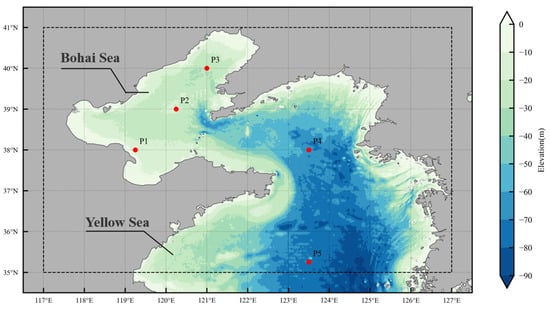
Figure 1.
Study area and selected locations map.
The bathymetric data used in this study include longitude, latitude, and depth values. The data were processed through grid-based interpolation, resampling the original discrete point data onto a regular grid. For missing values resulting from the interpolation, nearest neighbor interpolation was applied to fill the gaps, ultimately generating a continuous bathymetric field. The spatial resolution of the processed bathymetric data is consistent with that of the ERA5 reanalysis dataset, facilitating alignment and comparative analysis with marine environmental variables. Depth values are expressed in meters (m) with negative values indicating depths below sea level.
The two-dimensional wave spectrum data downloaded for this study contain wave energy information across different directions and frequencies. However, due to the high dimensionality of the 2D spectral features, regional-scale processing can be challenging. Directly using this data for modeling may result in increased computational complexity and data redundancy. Therefore, to reduce feature dimensionality and improve model feasibility, this study applies dimensionality reduction to the spectral data and utilizes one-dimensional frequency spectrum data for experimental analysis. The one-dimensional spectrum is obtained by integrating wave energy across all directions, preserving the frequency dimension while effectively representing key spectral characteristics with reduced data complexity.
2.2. Physical Analysis
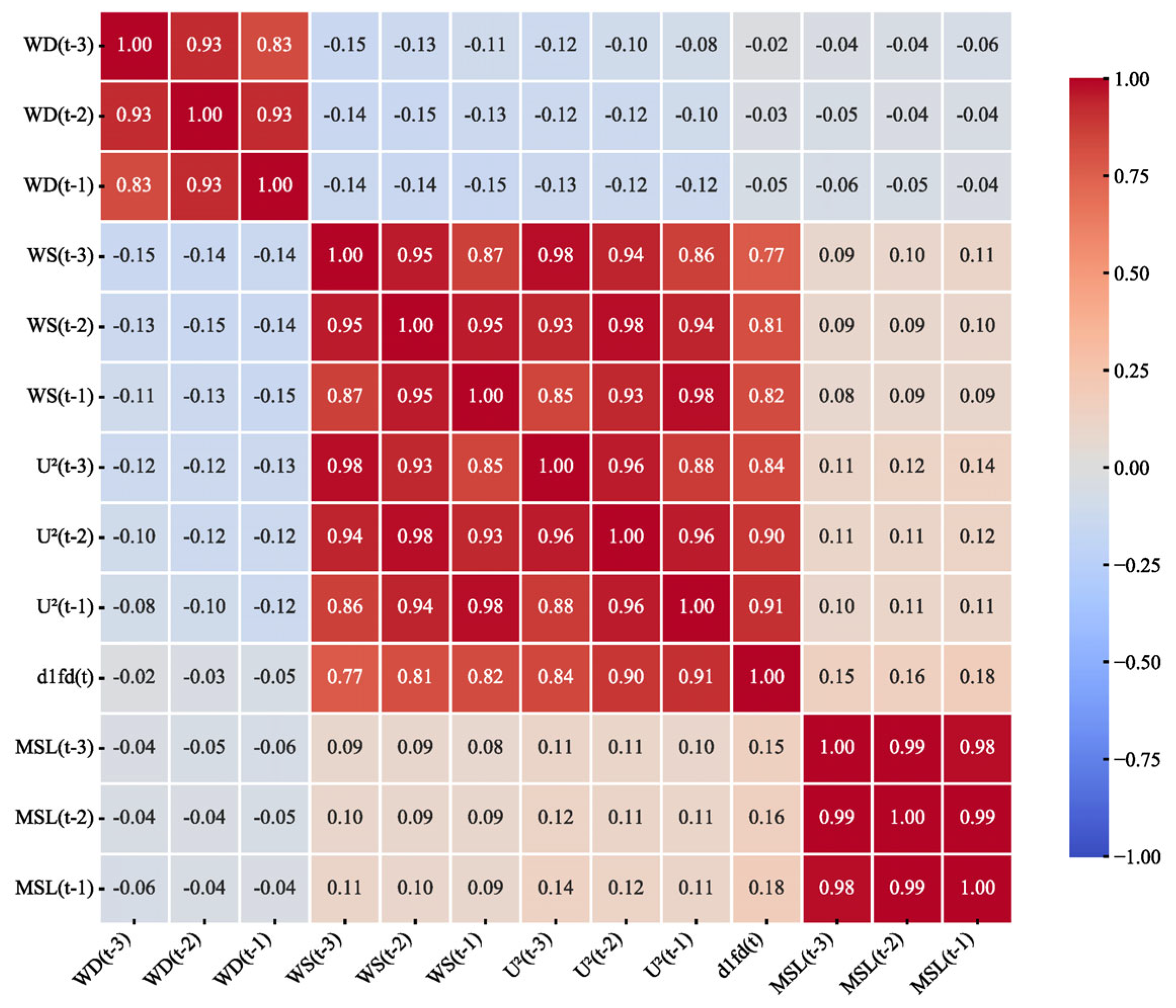
The generation and propagation of wave energy are directly or indirectly related to various meteorological and oceanographic factors. In this study, we analyze the influence of wind speed (WS), wind direction (WD), wind speed squared (U2), and mean sea level pressure (MSL) on wave growth at different lag times. In Figure 2, the Pearson correlation coefficients between meteorological factors and the one-dimensional spectral data, denoted as d1fd(t), are calculated. Here, d1fd(t) refers to the one-dimensional frequency-directional spectrum at time t, which is obtained by integrating over directional components. The time interval between t and the meteorological factors is 3 h, which is consistent with the temporal resolution of the input dataset. Wind speed is positively correlated with the one-dimensional spectrum at different times (0.77–0.82), which aligns with the physical mechanism that wind speed is a primary driving factor for waves. Wind speed is the primary driving force of wave generation and growth, as it transfers energy to the ocean surface. Continuous pressure is exerted on the wave surface, allowing energy to be effectively transferred into the water body, which results in the progressive increase in both wave height and wave length. Wind speed squared has a strong positive correlation with the spectrum (0.9) because energy is proportional to the square of velocity. Wind speed squared serves as a direct representation of wind energy, while the spectrum reflects the energy transfer process of waves. The correlation between mean sea level pressure and wave spectrum is relatively low (0.18); as a large-scale meteorological element, the pressure field does not directly affect the growth process of the wave spectrum. However, it can change the evolution of weather systems, thereby influencing the fetch and duration of the wind, which in turn affects the distribution characteristics of the wave spectrum. Additionally, in deep water, wave energy is more dispersed, allowing for relatively smooth propagation, while in shallow water, the same wave energy is compressed into a smaller area, leading to more concentrated energy transfer and faster energy loss. Therefore, the impact of water depth on the wave energy transfer process in the study area cannot be ignored.

Figure 2.
Pearson correlation heatmap of meteorological and wave parameters.
2.3. Method
2.3.1. CNN
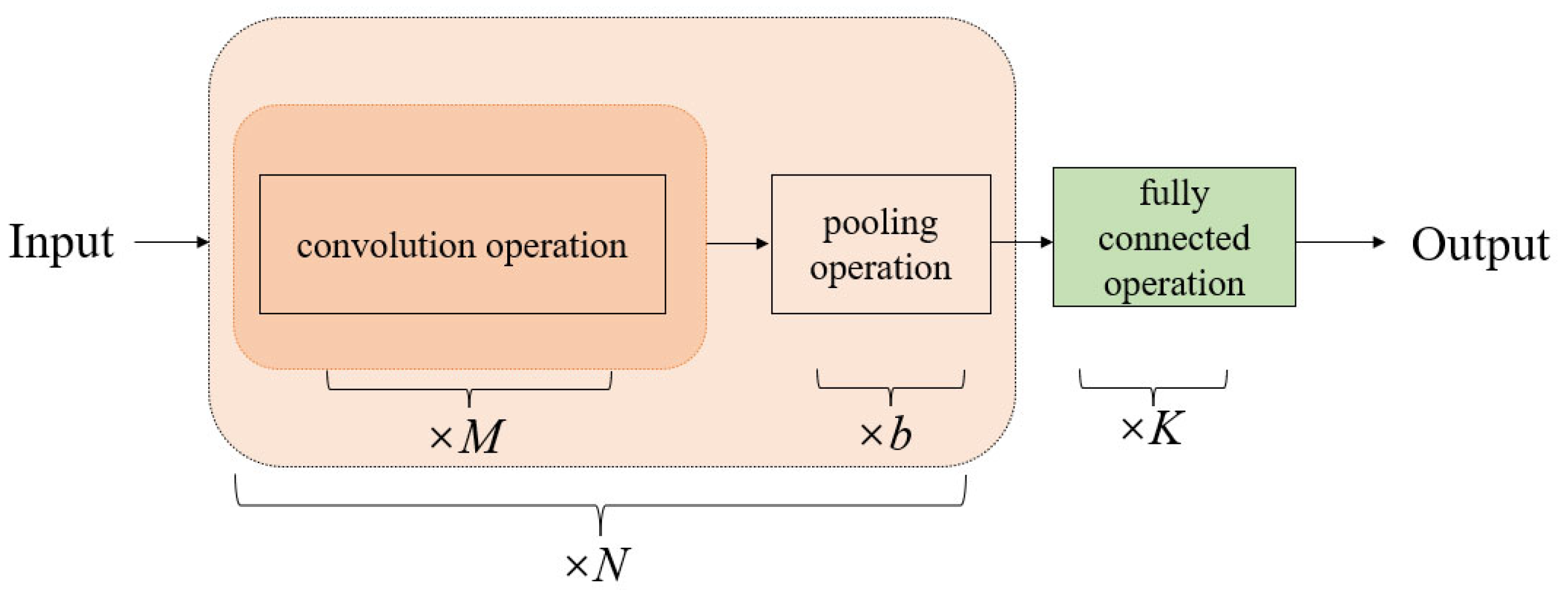
Convolutional Neural Networks [25] are a class of deep neural networks typically composed of an input layer, convolutional layers, pooling layers, and fully connected layers. In Figure 3, convolution operations are applied to the input data to extract features and generate feature maps. To capture features at different levels, convolution kernels of varying sizes are employed to detect multi-scale patterns within the input signals, resulting in multiple feature maps.

Figure 3.
CNN Model architecture.
Pooling operations are usually performed after convolutional layers, which is primarily to reduce the spatial dimensions of the feature maps while retaining essential information. Pooling layers downsample the feature maps to reduce the amount of data while preserving important features. Common pooling methods include max pooling and average pooling. Max pooling selects the maximum value within a specified window as the representative feature [26], whereas average pooling computes the arithmetic mean of all elements in the window to represent the features of the region.
In CNN, multiple convolutional and pooling layers are typically connected in an alternating fashion, enabling the model to progressively extract deeper and more abstract features. By stacking these layers, the model can learn hierarchical representations of the input data and extract richer feature information [27]. Finally, the fully connected layer further processes the features extracted through the convolution and pooling operations. The can be defined by Equation (1).
In the equation, denotes the input to the convolutional layer, represents the output feature map of the layer, is the weight matrix for convolution, denotes the element-wise multiplication (Hadamard product), is the bias vector, and is the activation function. The calculation for the pooling operation is defined by Equations (2) and (3).
In the equation, denotes the max pooling function, represents the bias, and denotes the output of the max pooling layer. The feature maps obtained through the pooling operation are then passed to the fully connected layer, which calculates the final output vector. The calculation for the operation is defined by Equation (4).
In the equation, denotes the final output vector, represents the bias, and is the weight matrix.
2.3.2. xLSTM Model
As an extension of the traditional LSTM, the extended Long Short-Term Memory network (xLSTM) addresses the limitations in memory capacity, information updating, and computational efficiency. In Figure 4, xLSTM introduces two main variants: sLSTM and mLSTM. Its key innovations include an exponential gating mechanism and a new memory structure that enhances the model’s ability to capture long-term dependencies while improving computational performance. Additionally, xLSTM incorporates residual blocks, allowing multiple xLSTM units to be stacked via residual connections, which ensures stable gradient propagation even in deep network structures. These improvements make xLSTM more efficient and robust for long-horizon time series forecasting tasks.
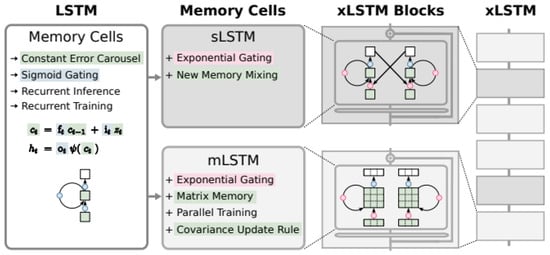
Figure 4.
xLSTM Model architecture.
- scalar LSTM
The sLSTM model introduces an exponential activation function into the input and forget gates, thereby implementing an exponential gating mechanism. This allows the forget gate to perform exponential weighting, making the retention and discarding of information more flexible. Additionally, a normalized state is incorporated, which adds the product of the input gate and all future forget gates to improve the model’s performance in handling long-term dependencies.
The sLSTM also employs multiple memory cells [28] and enables information blending across cells through recurrent connections. This enhances the expressive power of the model while maintaining low computational complexity.
The state update rules for an sLSTM memory unit at time step t are defined by Equations (5)–(14):
Cell state update:
Normalized state update:
Hidden state update:
Cell input:
Input gate:
Forget gate:
Output gate:
To prevent numerical overflow caused by the exponential activation, sLSTM also introduces steady-state gate [29] to replace and
In the Equations, represents the input vector at time step , and , denote the hidden and cell states, respectively. The gates , , and control the information flow. , , and are the learnable weights and biases for each gate.
- 2.
- matrix LSTM
Compared to sLSTM, the mLSTM further enhances memory capacity by extending the traditional vector-based memory units to matrix memory structures. This allows the model to capture more complex relationships within a single time step, improving both memory storage and information retrieval efficiency. While traditional LSTMs use scalar memory units, which may lead to information loss in long-term dependencies, mLSTM—drawing inspiration from Bidirectional Associative Memory Systems (BAMS) [30,31,32]—applies a matrix-based memory structure and a covariance update rule [33,34] to significantly boost storage capability. Additionally, mLSTM supports multiple memory cells and multi-heads, where each head functions as an independent memory-retrieval unit. This enables the model to capture information across multiple temporal scales simultaneously, improving computational efficiency and scalability for large-scale datasets.
The state update rules for an mLSTM memory unit at time step t are defined by Equations (15)–(23):
Matrix state update:
Normalized state update:
Hidden state update:
Query input:
Key input:
Value input:
Input gate:
Forget gate:
Output gate:
In the equation, denotes the matrix form of the cell state, and represent the value vector and key vector, respectively, and represents the query vector used for retrieval.
2.4. Evaluation Functions
We defines the Mean Absolute Error (MAE), Mean Absolute Percentage Error (MAPE), Root Mean Square Error (RMSE), Spatial Average Root Mean Square Error (SARMSE) and Bias to evaluate the accuracy of the model’s predictions. The calculation methods for these three metrics are shown in Equations (24)–(28).
In the formula, i and j represent the coordinates of the data grid points, k denotes the time step of the output data, N is the total number of data grid points that meet the conditions, I is the total number of longitude grid points, J is the total number of latitude grid points, K is the total number of output data points, and R is the ratio of the marine area within the study region to the total area. This allows the focus to be on the error in the marine portion. represents the one-dimensional frequency spectrum predicted by the CNN-XLSTM model at a specific point in the study area, while represents the one-dimensional frequency spectrum from the ERA5 dataset at a specific point in space and time.
3. Model Structure
3.1. Experimental Framework
To clarify the overall experimental framework, we first construct the prediction model and introduce the architecture and functions of each module. Subsequently, we design different input variable combinations to build multiple datasets for comparative evaluation. To assess the effectiveness of our proposed model, we conduct benchmark experiments against several representative deep learning methods. Based on the results of wave spectrum and spectral parameter analysis under different input settings, we identify the optimal model configuration for further study.
3.2. CNN-xLSTM Network Model
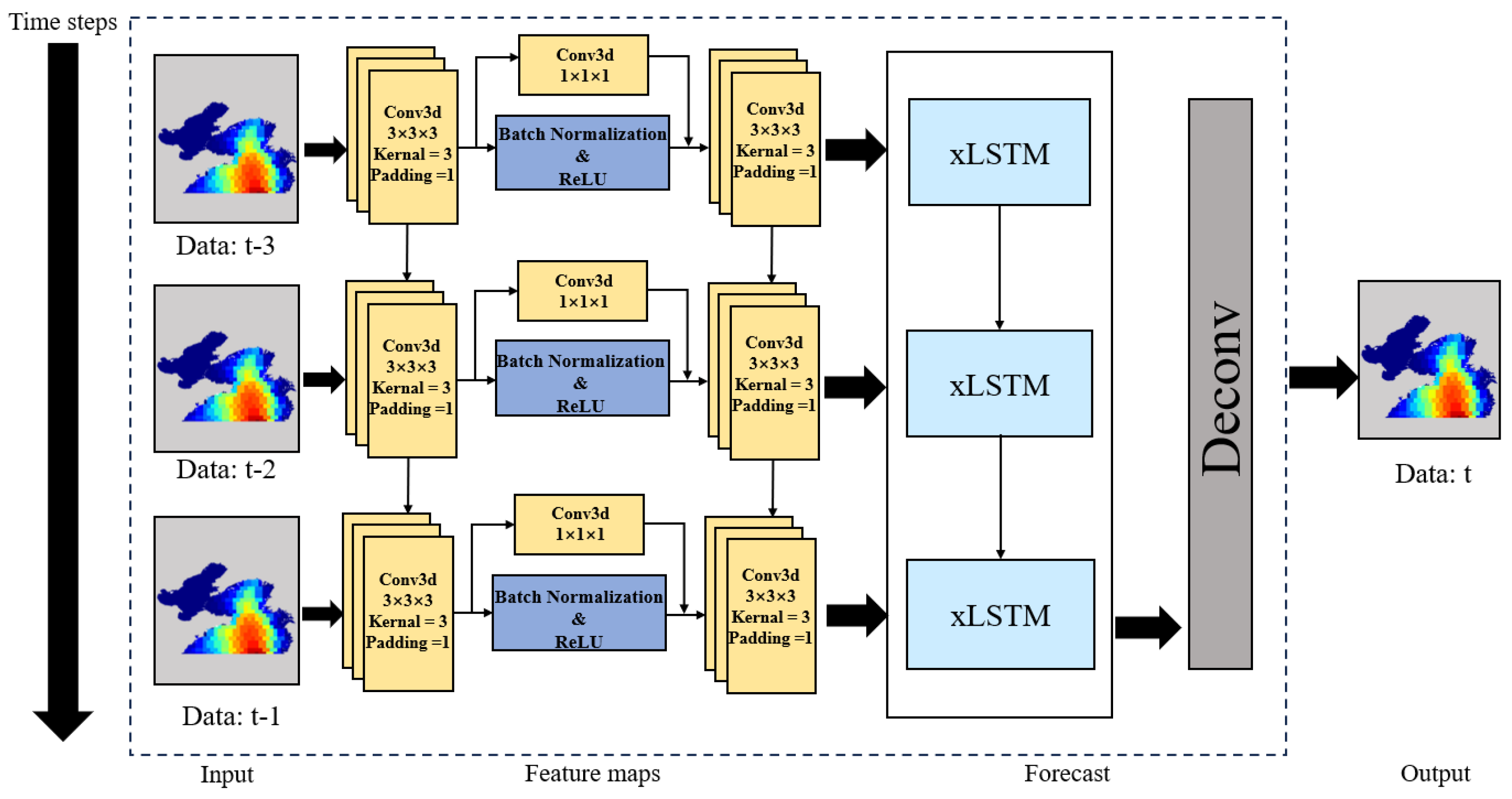
This paper establishes a regional wave spectrum prediction model based on the CNN-xLSTM network. It uses one-dimensional frequency spectra from three consecutive time steps and wind speed as the basic input data. The one-dimensional frequency spectrum data for a future time is captured through three layers of Conv3D layers; then, the feature dimensions are adjusted through a fully connected layer before being input into the xLSTM for prediction. Finally, a deconvolution layer adjusts the feature dimensions and outputs the one-dimensional frequency spectrum data for a future time. The model is illustrated in Figure 5. For example, inputs from 00:00, 03:00, and 06:00 on 1 January 2020 are used to predict the wave spectrum at 09:00. These three time steps are stacked into a tensor. A 3D convolution is then applied across the temporal and spatial dimensions to extract local spatiotemporal features.
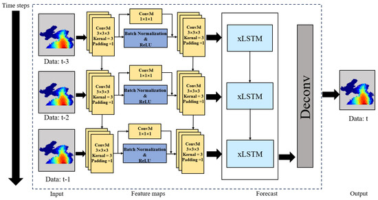
Figure 5.
Overall model architecture.
We use Conv3D instead of Conv2D for feature mapping because Conv3D can perform convolution operations in both spatial and temporal dimensions. Conv2D can only convolve in the height and width spatial dimensions; it is unable to capture variations in the temporal dimension. To ensure that feature mapping retains more original information and feature distribution, Batch Normalization (BN) [35] layers are employed after each convolution to standardize feature distribution. After the first convolution, a residual connection is added to preserve the initially extracted features and enhance the model’s feature representation capability, avoiding feature reduction caused by pooling layers. To improve the model’s ability to capture nonlinear features, a Rectified Linear Unit (ReLU) is used as the activation function in each layer. The convolution kernels are set to 3 × 3 × 3, 3 × 3 × 3, and 1 × 1 × 1 to capture different features at various spatial scales. The third Conv3D (1 × 1 × 1) is used in the residual branch to match dimensions for addition. During the xLSTM, input data undergo Layer Normalization (LN) [36] and include a dropout layer (p = 0.2) to prevent overfitting and enhance model stability. For model training, Smooth L1 is used as the loss function, which provides more stable training and reduces the impact of outliers compared to RMSE and MAE. The number of iterations is set to 100 while keeping other parameters unchanged. All experiments in this study were conducted on a Linux server equipped with an Intel(R) Xeon(R) Platinum 8352V CPU (16 cores, 2.10 GHz), an NVIDIA RTX 4090 GPU with 24 GB of memory, and 120 GB of RAM (Santa Clara, CA, USA). The models were implemented using the PyTorch 1.10.0 deep learning framework. Additional Python libraries such as NumPy 1.21.6 and Pandas 1.3.5 were also utilized during the experiments.
3.3. Dataset Construction
In this study, the performance of the prediction model depends not only on the settings of hyperparameters but also on different input data; thus, it is necessary to consider the correlations between different inputs. Based on the Pearson correlation coefficients analyzed in Figure 2, we introduce additional factors—10 m u-component of wind (U10), 10 m v-component of wind (V10), wind speed squared (U2), mean sea level pressure (MSL), and water depth (DEP)—to better characterize the features of wave fluctuations. Six models were established based on different input combinations. Model A is a direct prediction model using d1fd, U10, and V10 as inputs. Model B includes the U2 in addition to the inputs of Model A. Model C considers the impact of MSL on wave spectra, adding MSL to the inputs of Model A. Model D accounts for the influence of DEP on wave generation and propagation, adding DEP to the inputs of Model A. DEP is a key factor in determining whether large waves can form in a particular area [37]. Model E combines the effects of both DEP and MSL, adding both DEP and MSL to the inputs of Model A. Model F further adds U2 to the inputs of Model E. Table 2 summarizes the inputs and outputs for each model.
Table 2.
Input selections for different models.
3.4. Model Comparison
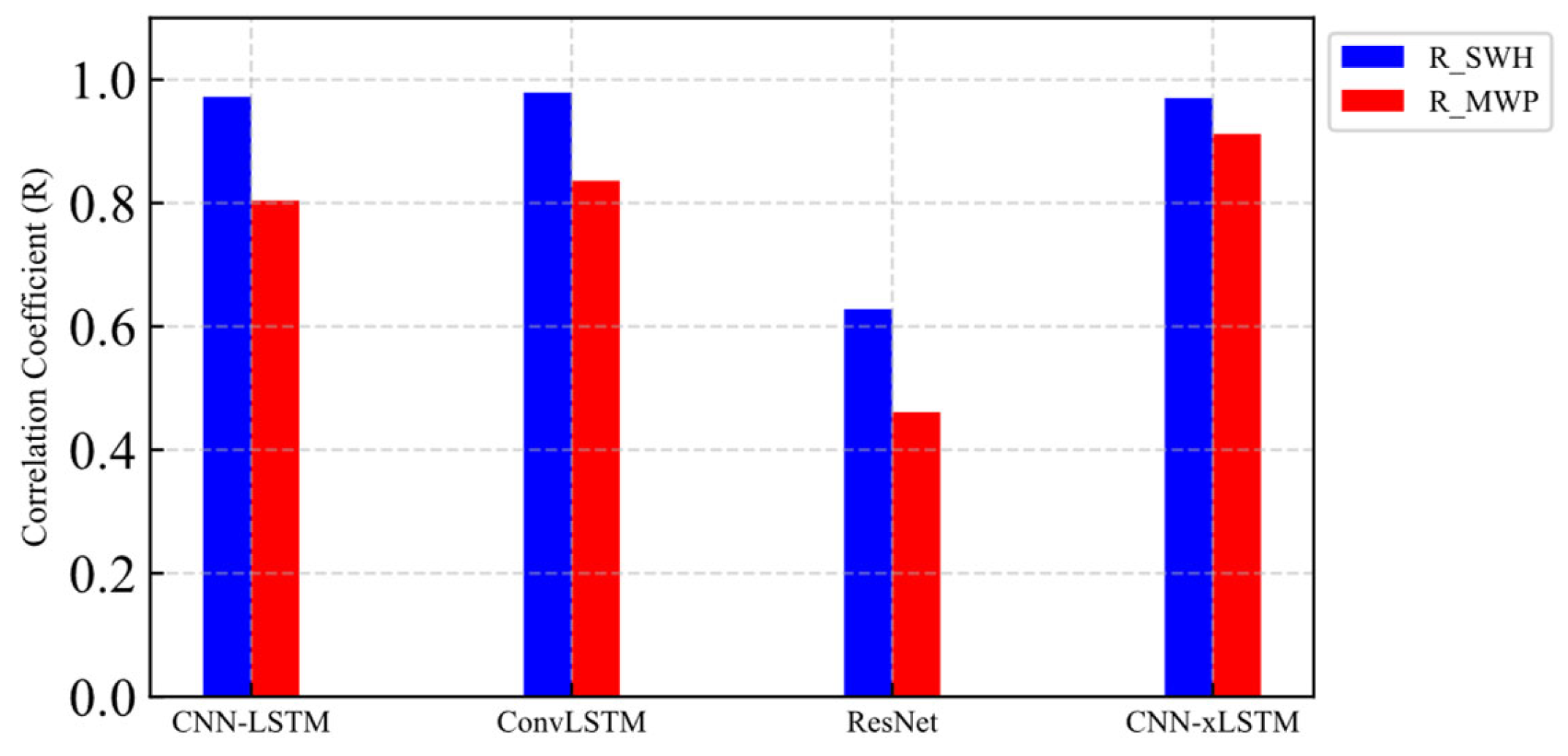
To evaluate the performance of different models in wave prediction tasks, we selected ResNet50 as a representative of typical convolutional neural network structures and introduced CNN-LSTM and ConvLSTM models with temporal modeling capabilities for comparison alongside our proposed CNN-xLSTM model. All models were trained using the SmoothL1 loss function and the Adam optimizer with 100 training epochs and a learning rate of 0.0002. All input data are from Model A. Figure 6 and Table 3 present the performance comparison of the four models on the test set; based on the predicted spectrum, the integral formula is used to obtain the results of SWH and MWP. The results show that the CNN-xLSTM model performs slightly lower in terms of SWH, the performance remains within an acceptable range, and it achieves the best performance in MWP prediction. This indicates that the proposed model has a certain advantage in capturing the spatiotemporal features of wave spectra.

Figure 6.
Comparison of correlation coefficients between significant wave height and average period for different models.
Table 3.
Comparison of the Performance of Various Models.
3.5. Model Selection
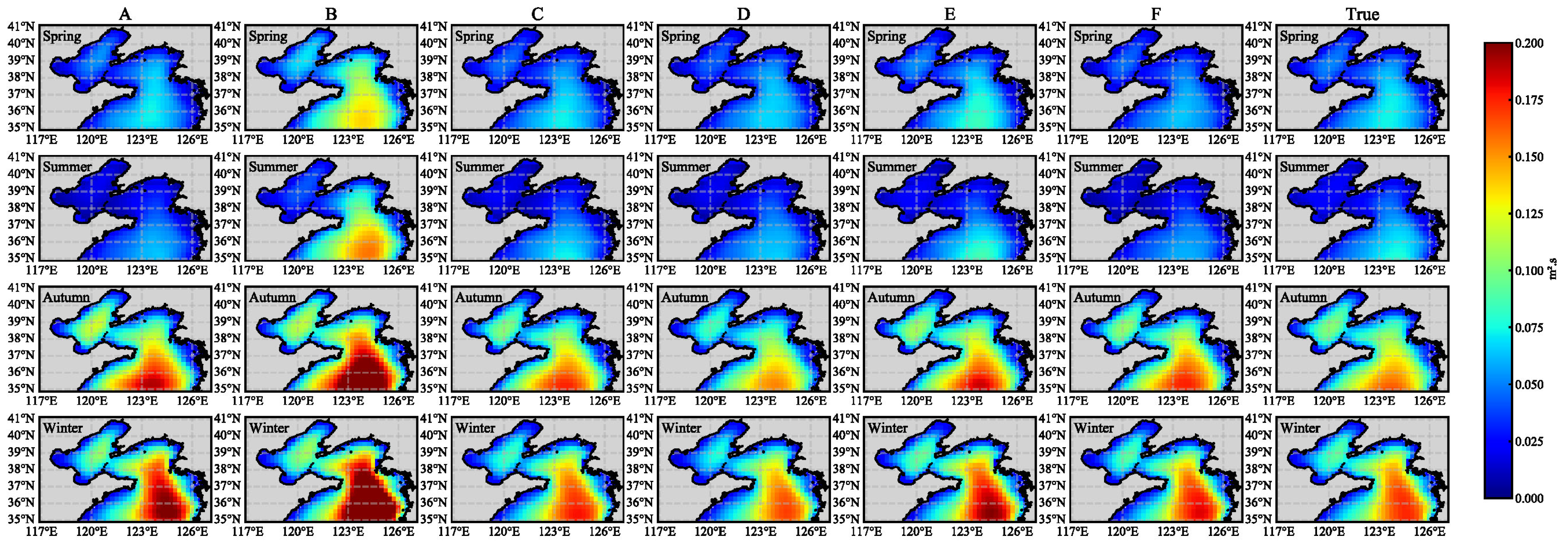
To evaluate the prediction performance of each model under different combinations of input features, the overall seasonal variation trends of all models were observed from a spatiotemporal perspective. The mean spatial distribution of spectral energy for ERA5 ground truth and model predictions in spring (March–May), summer (June–August), autumn (September–November), and winter (December–February) is shown in Figure 7A–F. From the spatial distribution patterns, Model B shows a significant overestimation of energy in spring and summer, with numerous anomalously high values appearing in the northern and central Yellow Sea, deviating considerably from the true spectra. Model A tends to overestimate in parts of the central Bohai Sea during autumn and winter, and it fails to capture the high-energy regions effectively in summer. In contrast, Models C, D, E, and F exhibit higher consistency with the ground truth in terms of seasonal spatial structure, demonstrating better spatial fitting ability and seasonal adaptability.
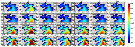
Figure 7.
Comparison of seasonal spatial wave energy predictions and ground truth for different models.
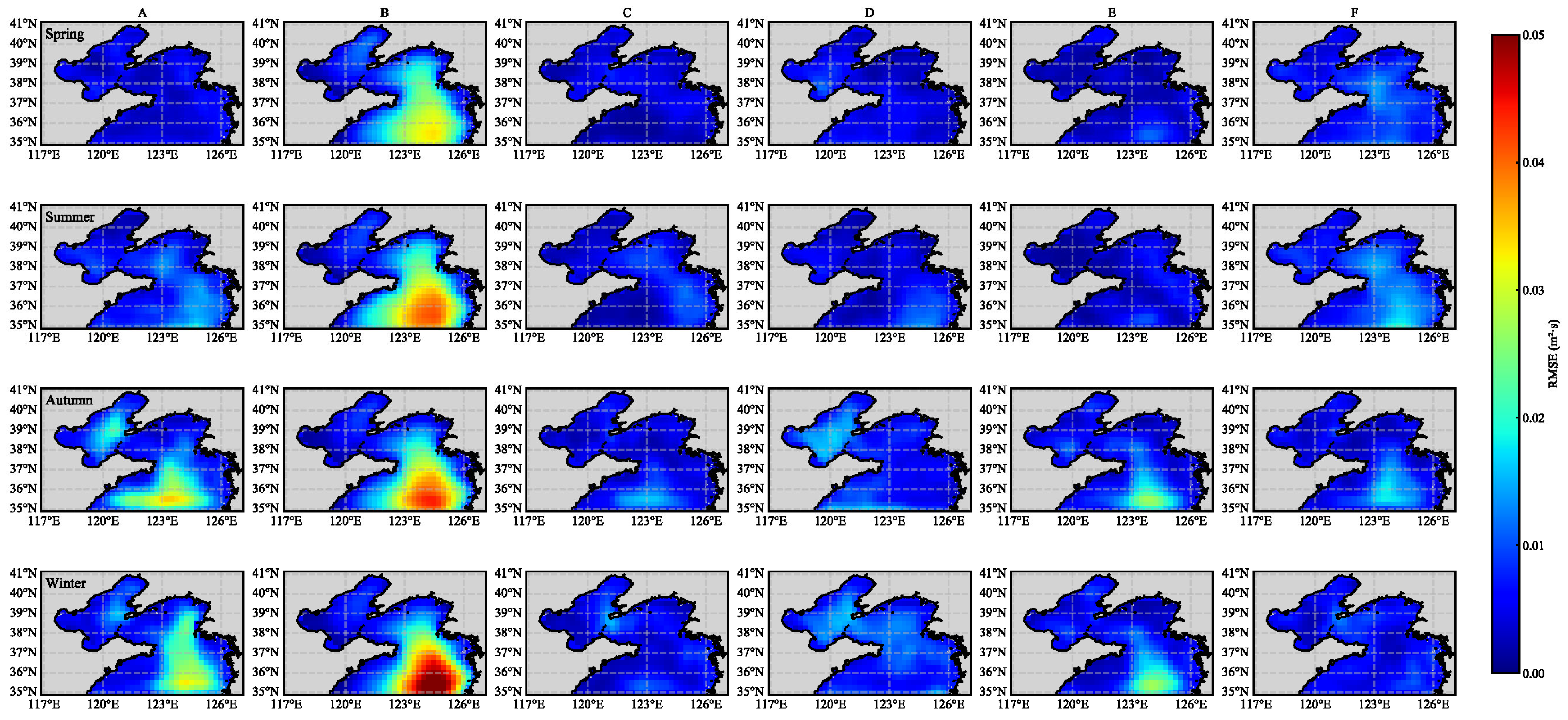
Further analysis was conducted by combining Table 4 and the seasonal spatial distributions of the overall spectral energy RMSE, as illustrated in Figure 8A–F. Each column corresponds to a model, and each row represents a season. Lighter colors indicate lower regional prediction errors. In terms of overall trends, Models A and B exhibit large spatial errors. Models C, D, and E generally show lower errors in the Bohai Sea and northern Yellow Sea; however, Model D displays slightly higher errors in the Bohai Sea during autumn and winter, while Model E shows slightly elevated errors near the boundary of the central Yellow Sea in the same seasons. Model D achieves the lowest seasonal SARMSE in spring and summer (spring: 0.022 m2·s, summer: 0.019 m2·s), indicating strong fitting ability under stable wave conditions. Model C maintains low errors in both spring and autumn, suggesting stable performance under varying sea conditions. In contrast, although Model E does not yield the lowest error in any single season, it consistently maintains relatively low and stable errors across all seasons (spring: 0.024 m2·s, summer: 0.020 m2·s, autumn: 0.040 m2·s, winter: 0.035 m2·s), with a more balanced spatial error distribution and no widespread high-error regions. Model D achieves the lowest SARMSE in each season, while Model C demonstrates stronger cross-seasonal stability. For Model E, most of the spatial errors are located near the boundaries of the study area, which are inevitably influenced by swell from outside the region. Therefore, analyzing spectral distribution alone is insufficient to determine the optimal model. It is also necessary to incorporate a sensitivity analysis of key oceanic and meteorological variables within the region to identify the most representative model architecture.
Table 4.
Seasonal SARMSE of spectral energy for different models.
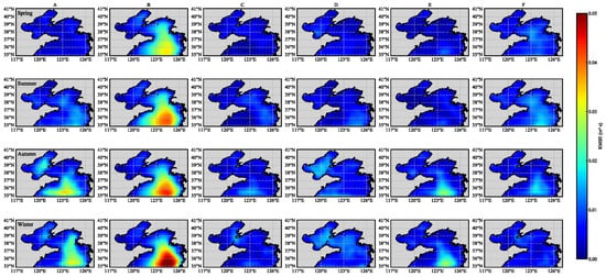
Figure 8.
Spatial distribution of RMSE between predicted spectra and ERA5 ground truth across seasons for different models.
To further validate the prediction results from a statistical perspective, we also compare the integral wave parameters, including SWH and MWD, which are both calculated from the ERA5 spectra and the model-predicted frequency spectra (the definitions of these parameters are provided in the Appendix A). Table 5 shows the error indicators of wave parameters for different models in the region. The MAPE is calculated based on regular sea states with MWP values greater than 3 s and SWH values above 0.5 m in order to exclude minor wave conditions. By comparing the error metrics for SWH and MWP, Models A and B exhibit excessive errors and are therefore excluded from further analysis. Model C and Model D, which incorporate MSL and DEP, respectively, both show notable performance improvements. The SWH RMSE decreases to 0.138 m and 0.141 m, respectively, with MAPE values of 13.24% and 15.68%. Model E considers both sea level pressure and water depth simultaneously, and it achieves the best overall performance: the RMSE for SWH was 0.138 m, and the RMSE for MWP was reduced to 1.331 s. In contrast, Model F does not improve performance; instead, it increases the error, suggesting that redundant features may interfere with model learning. Taking into account the seasonal SARMSE statistics, although Model E shows a slightly higher SARMSE, its improved accuracy in key variable prediction makes it more suitable for practical applications. Therefore, Model E is selected as the baseline for subsequent comparisons.
Table 5.
Analysis of regional marine element metrics for different models.
To further validate the effectiveness of our model, we compared it with the CNN-based method for predicting SWH in the Bohai Sea and Yellow Sea [38]. After obtaining the predicted spectral values, the SWH is derived using the integration formula and divided into four SWH intervals. As shown in Table 6, the model has low errors in most intervals, especially above the mid-wave range, indicating that the model is competitive.
Table 6.
Compare MAE under different SWH intervals using different methods.
4. Results and Discussion
4.1. Regional Wave Spectrum Characteristics Analysis
4.1.1. Comparative Analysis of SWH Prediction: Spectrum-Driven vs. Direct Significant Wave Height Input
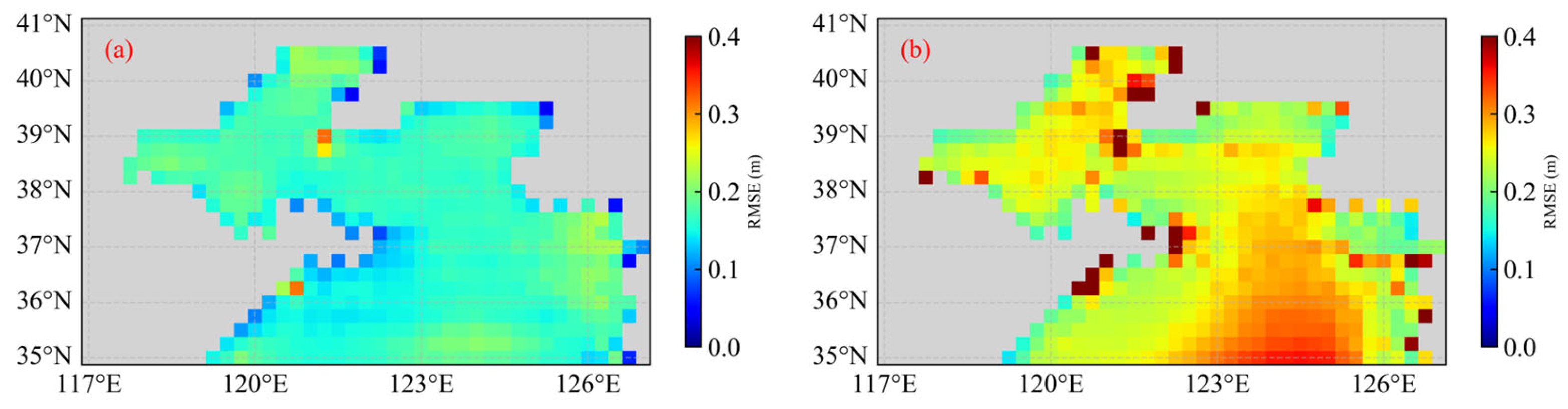
To verify the effectiveness of using wave spectra for SWH prediction, we constructed a baseline model that directly predicts SWH by replacing the spectrum input with SWH data while maintaining the same model architecture and hyperparameters. Using identical training and testing datasets, we compared the optimal results of the direct prediction model with those derived from the spectrum-predicted SWH calculated via standard spectral formulas. Figure 9 and Table 7 present the spatial RMSE distribution of SWH for both approaches. From both the spatial distribution and overall error metrics, the spectrum-driven model clearly outperforms the direct significant wave height model in terms of prediction accuracy. The RMSE, MAE, and MAPE of the spectrum-driven model are 0.138 m, 0.078 m, and 13.17%, respectively, while those of the direct SWH prediction model are 0.251 m, 0.124 m, and 27.15%. This superiority may be attributed to the richer nonlinear information embedded in the wave spectrum, which contains the frequency components and energy distribution of ocean waves. Additionally, Wang et al. [39] noted that the Bohai and Yellow Seas are typical enclosed or nearshore regions where complex topography and land–sea boundary effects increase model uncertainty. Their comparison with buoy observations showed errors concentrated around 0.2 m, further supporting the practicality of the method proposed in this study.

Figure 9.
Spatial RMSE distribution of predicted significant wave height: (a) the spectrum-based prediction method; (b) the direct significant wave height prediction method.
Table 7.
Performance metrics of significant wave height prediction.
4.1.2. Seasonal Analysis of Regional Wave Spectra
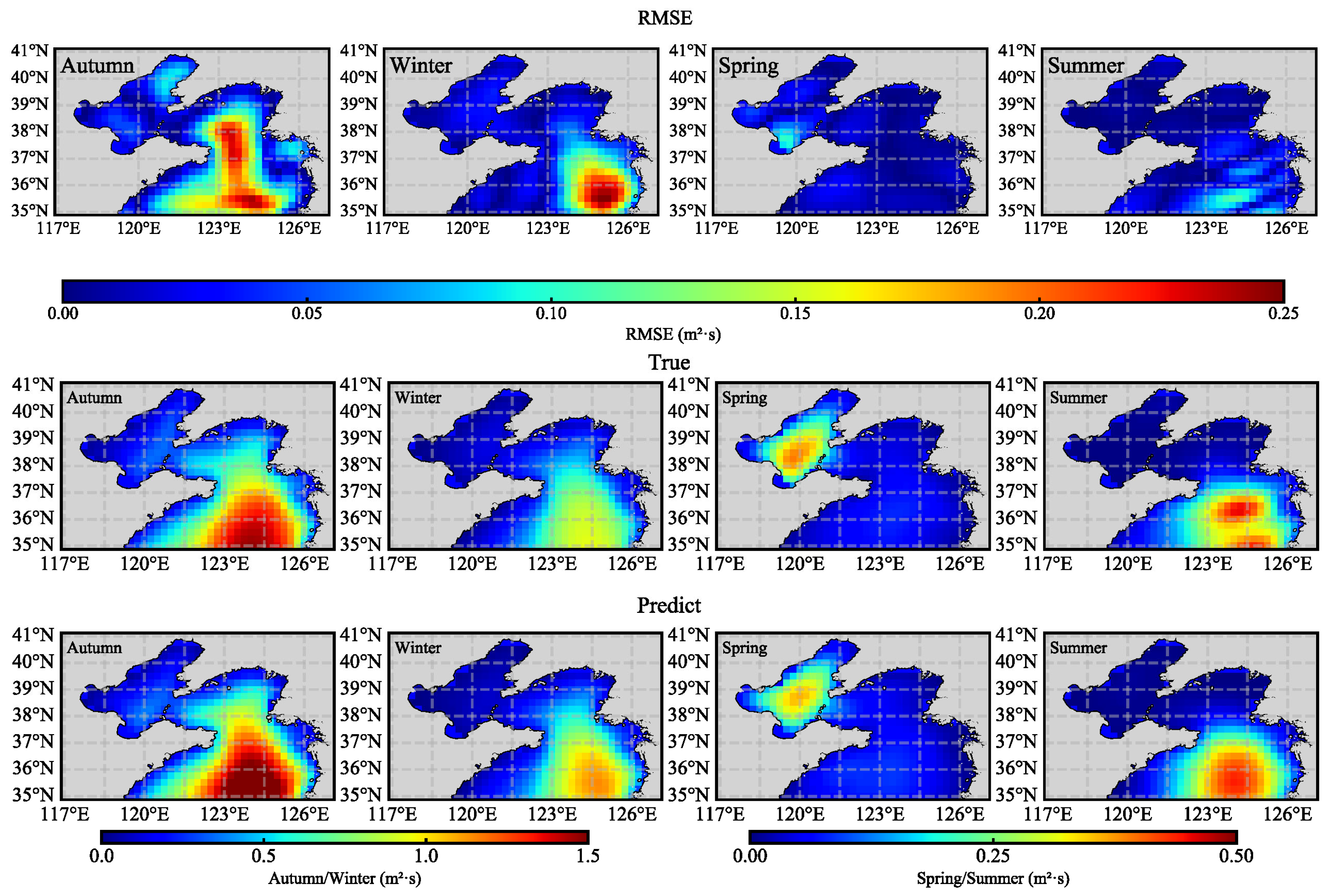
The spatial distribution characteristics of the spectrum exhibit significant seasonal variations. To elucidate the distribution patterns of spectral energy across different seasons, we identified moments of maximum SWH and wind speed during the four seasons—spring (March–May), summer (June–August), autumn (September–November), and winter (December–February)—as representative nodes. Additionally, we accounted for potential interference that could arise at the junction of seasons by selecting temporal points that accurately reflect changes in spectral energy within each season.
In Figure 10, during spring (21 April 2022), the true spectral energy is mainly concentrated in the Bohai Sea with the primary errors located near the coast of Laizhou Bay. The corresponding SARMSE in Table 8 is 0.048 m2·s. In summer (13 July 2022), the spectral energy is primarily distributed in offshore deep-sea areas, showing smooth variations; the SARMSE is 0.040 m2·s, indicating that summer wave systems are more regular and the model can more easily capture their features. In autumn (16 October 2021), energy is concentrated in the Yellow Sea and the Korea Bay. While the model captures the overall pattern well, it significantly overestimates energy in the central Yellow Sea. The SARMSE is 0.142 m2·s, the highest among the seasons, which is likely due to greater sea–air temperature differences and enhanced pressure gradients in autumn, leading to more sustained wind energy input and higher spectral energy values. In winter (12 January 2022), spectral energy is generally centered in the mid-Yellow Sea with an SARMSE of 0.061 m2·s.
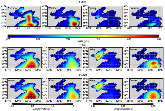
Figure 10.
Comparison of four seasons representative time points.
Table 8.
SARMSE at representative time points in each season.
4.2. Single-Point Wave Spectrum Characterization
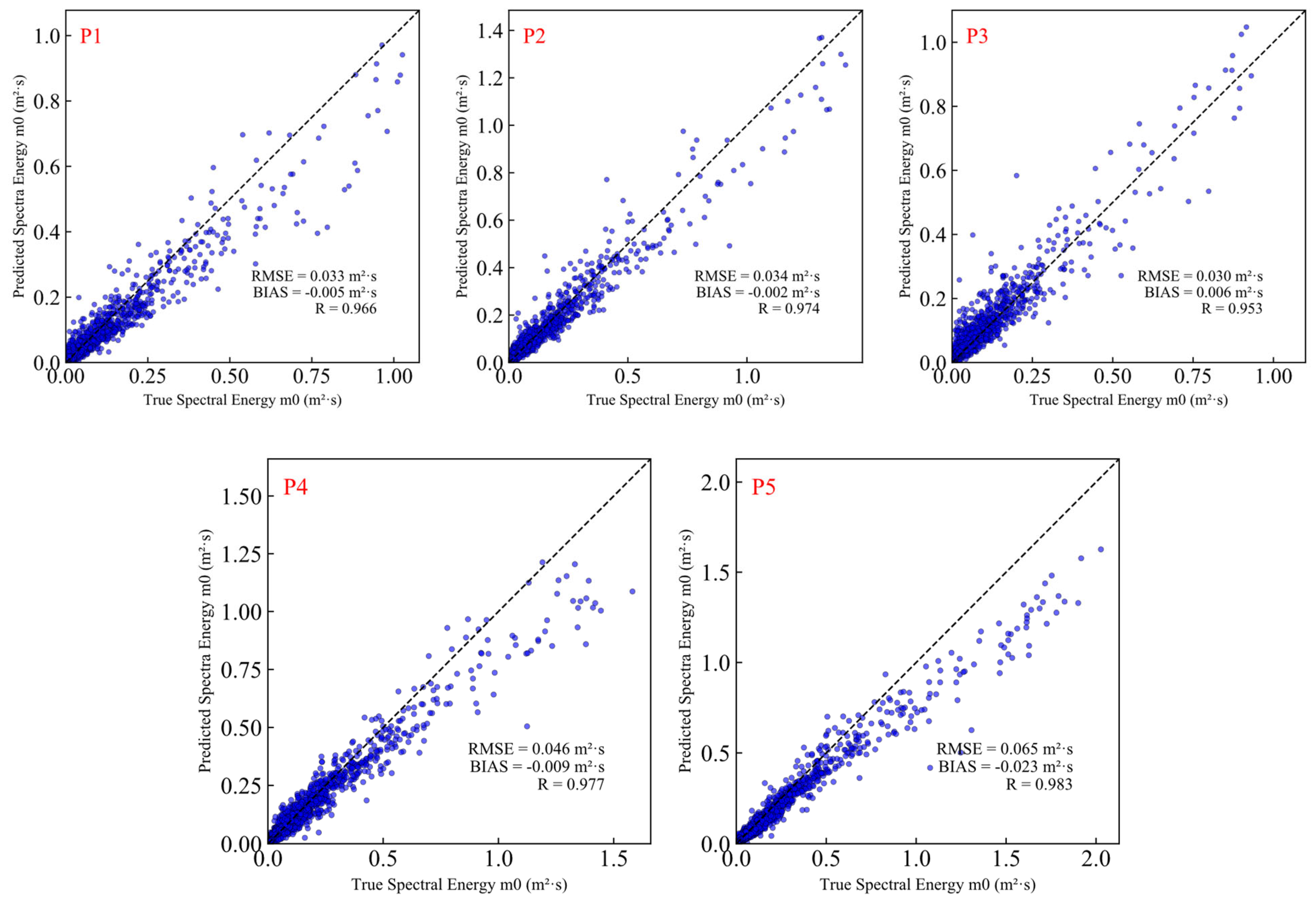
To validate the model’s performance in different regions, we select five points from Figure 1 as representatives. Point P1 is located in the nearshore area of the Bohai Sea, where the water depth is relatively shallow. This point is influenced by the land topography, and the wave propagation path is relatively long. Points P2 and P3 are located between the Bohai Sea and Liaodong Bay. These two points are controlled by the southward movement of cold air, where the wind direction and speed vary greatly, and they are often accompanied by atmospheric disturbance processes. Selecting these points helps to investigate the model’s ability to capture the response mechanisms under wind region variations. Point P4 is located in the northern Yellow Sea, and its selection aims to test the model’s predictive ability in semi-enclosed sea areas. Point P5 is located in the central Yellow Sea, close to the boundary of the study area, which is easily influenced by typhoons, remote swell waves, and other events. This point is chosen to evaluate the model’s ability in deep-water areas near the boundary and its response to remote wind field influences.
The scatter plots of the spectral energy M0 between the true values and predicted values at the five points are shown in Figure 11. The deviations are close to zero with the correlation coefficient (CC) ranging from the lowest (0.95) to the highest (0.98). The RMSE at point P5 is higher than at the other four points because it is located at the boundary of the study area and is influenced by remote swell waves from the southern region. Additionally, wave breaking and dissipation occur as the waves propagate northward. As indicated [40], closed and nearshore regions are more difficult to model compared to open sea areas. From the model’s perspective, the boundary area has fewer data, and the model is unable to access information outside the boundary. This leads to an insufficient understanding of the boundary extraction, and the evaluation metrics at the boundary area are more prone to error, which amplifies the overall mean error.
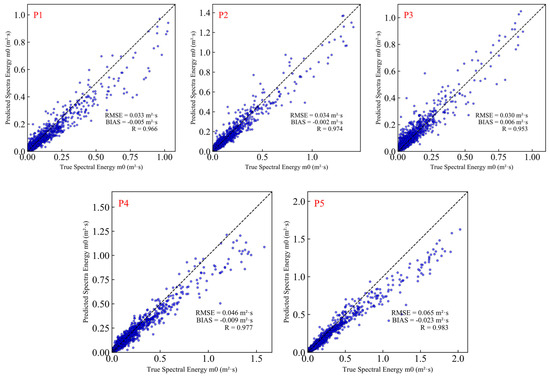
Figure 11.
Scatter plot for comparing RMSE, Bias, and R of the true and predicted wave spectra energy M0 at representative points in the test set.
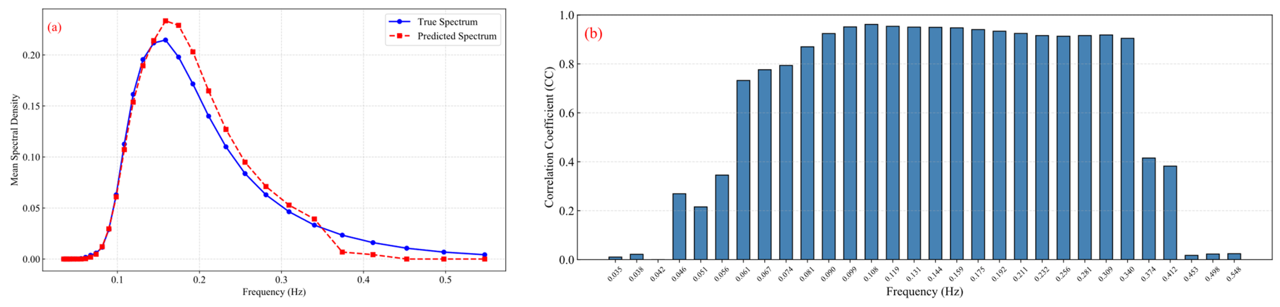
Figure 12a shows the average spectral energy density distribution with frequency across the entire study area, where the measured values are represented by the blue line and the model predictions are represented by the red line. From the figure, it can be observed that the model’s predicted spectral frequency is generally higher than the true values, and the high-frequency energy is underestimated and decays faster. In deep-sea areas, nonlinear interactions between waves can transfer energy from the spectral peak to the low-frequency range, which is an important characteristic of spectral evolution [41]. In the main frequency range of 0.1 Hz to 0.3 Hz, the model’s predicted energy is slightly higher than the true values, indicating that the model has some fitting ability. However, when the spectral peak shifts to the high-frequency range, the model fails to fully capture this nonlinear transfer, which could be the reason for the high-frequency bias in the predicted spectral peak. Moreover, in the energy transfer process, high-frequency components quickly dissipate, while long-wave energy supports wave growth [42], leading to a faster decay of the actual spectrum in the high-frequency tail. At the same time, neural networks tend to have spectral bias, favoring the fitting of low-frequency signals, and high-frequency components are often harder to learn [43]. Therefore, insufficient energy fitting in the high-frequency range is one of the errors in the current model’s prediction.
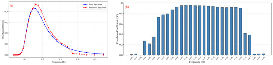
Figure 12.
(a) Average spectral density distribution of ERA5 true values and predicted values across the entire region. (b) Correlation coefficient between the model’s estimated spectral density and ERA5 spectral density at different frequencies in the validation set.
Figure 12b shows the CC of the model across different frequencies on the validation set. In the main frequency range from 0.1 Hz to 0.35 Hz, the CC is greater than 0.90, but the correlation is lower at both low and high frequencies. This is consistent with the average spectral density distribution shown in Figure 12a. Unlike the method in JIANG (2023), where the spectral prediction at a single point is trained from high to low frequencies on a per-band basis, we train the model as a whole. This approach works well in the main frequency range, but due to insufficient data in the low and high-frequency ranges, the model’s generalization ability is poor, and performance declines in the edge frequency bands. This is another reason for the errors observed.
This bias is also reflected in Table 9 and Table 10. In Table 9, the peak frequency, as the most representative and easily measurable variable in the one-dimensional frequency spectrum, changes slowly and can reflect the development stage of the waves. The RMSE for the five representative points is between 0.03 and 0.04, with the lowest peak frequency errors at P4 and P5, indicating strong temporal consistency in the dominant wave periods. However, combining with the spectral peak value errors in Table 10, it is evident that P4 and P5 have larger energy fluctuations with higher deviations in the predicted spectral peak values. This further indicates that while the model can predict the main frequency location well, it still has shortcomings in fitting high-frequency energy amplitudes.
Table 9.
Peak frequency evaluation metrics.
Table 10.
Spectral peak evaluation metrics.
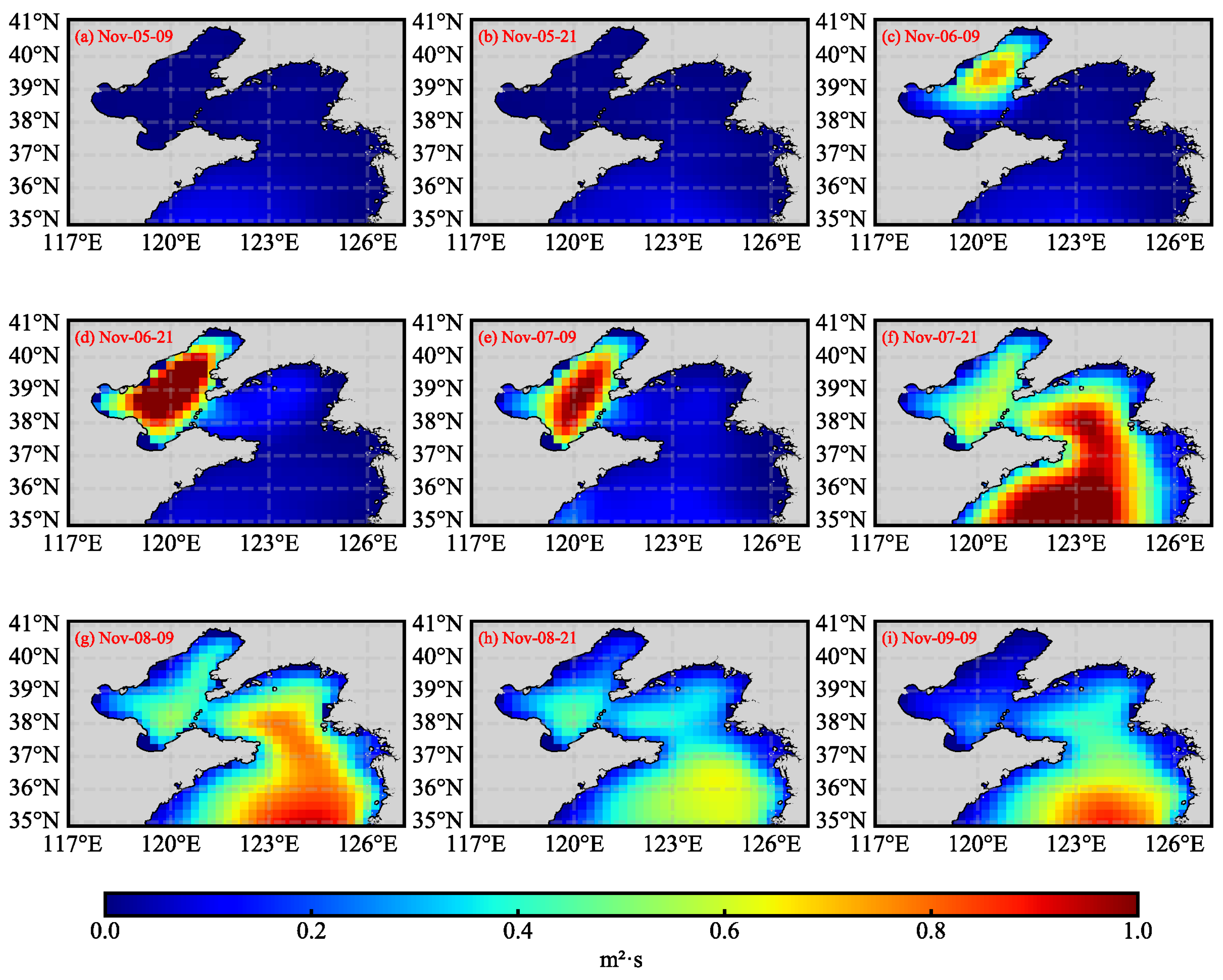
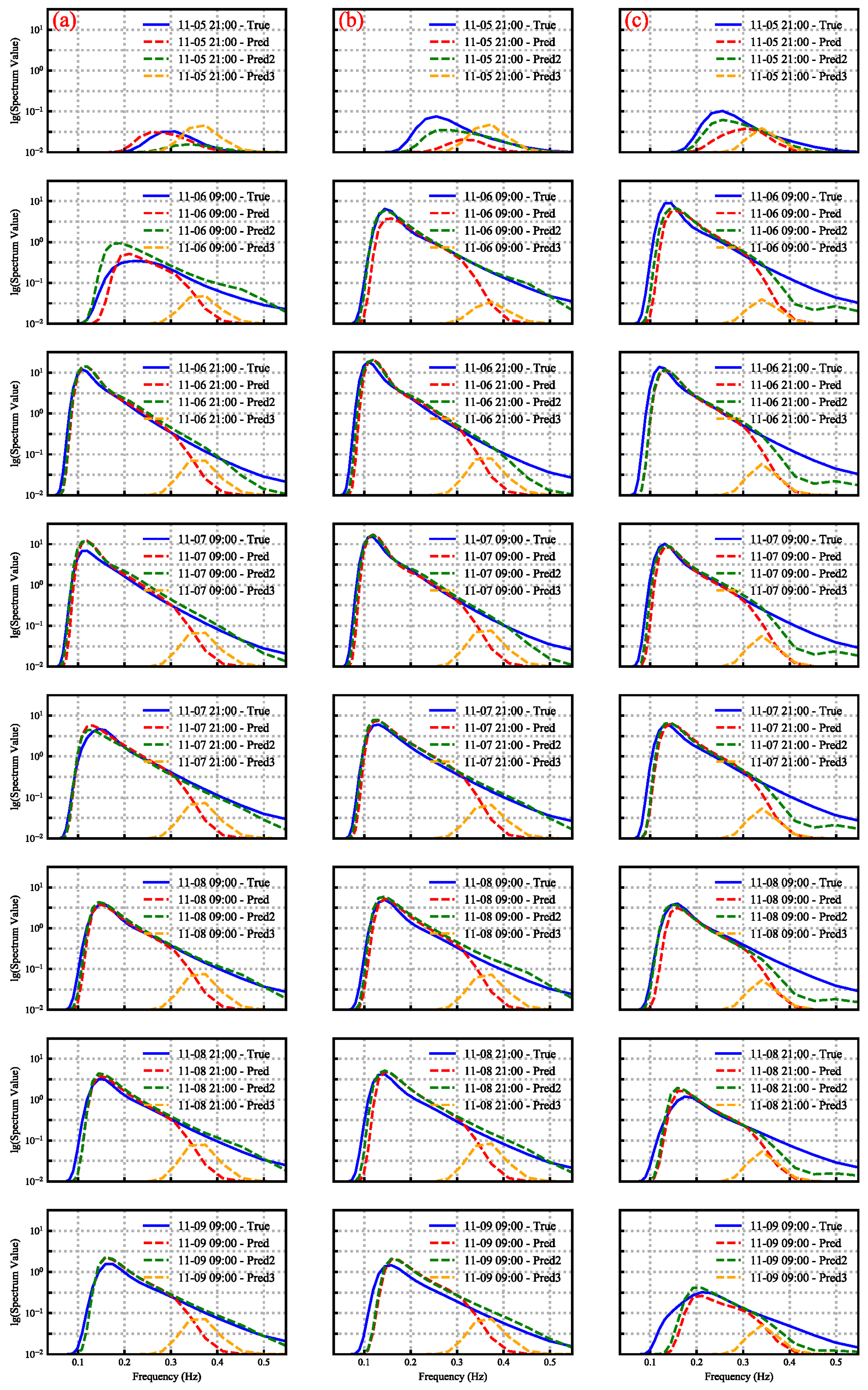
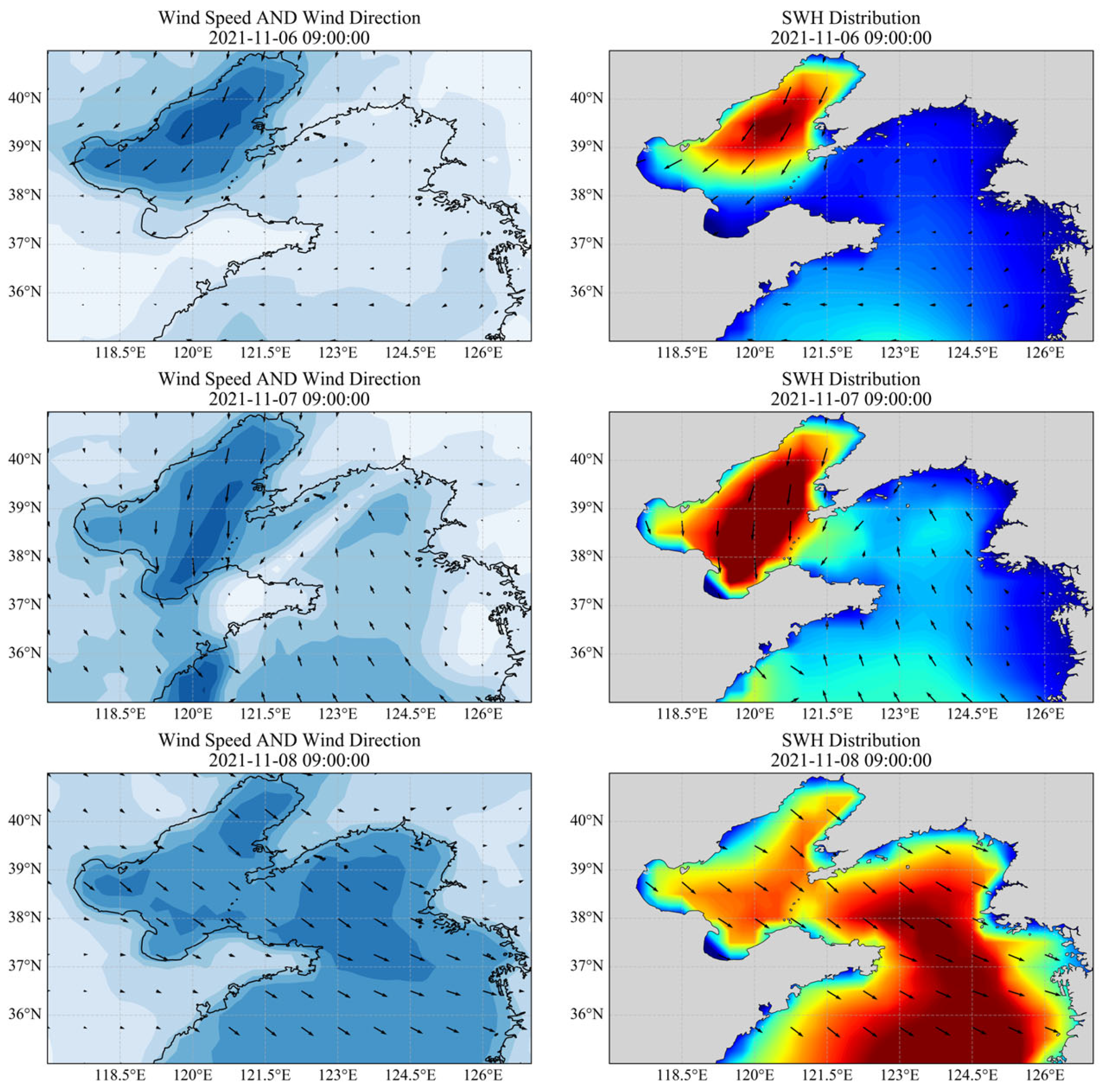
We select the wave characteristics of the Bohai Sea and its surrounding areas during the strong northern cold wave in early November 2021 as the research subject [44]. We combine the spatiotemporal variation characteristics of M0 during the cold wave (Figure 13) with the time-series wave spectrum at single points P1, P2, and P3 during the cold wave (Figure 14) for analysis. In Figure 14, the blue curve represents the ERA5 real data, and the red curve represents the predicted values. To clearly reflect the spectral variation, the y-axis is plotted using a logarithmic scale (log10). For comparison, the spatial distribution of wind speed, wind direction, and SWH is also shown in Figure 15.

Figure 13.
Variation of spectral energy m0 in the Bohai and Yellow Seas during the passage of a cold wave (with 12 h intervals).
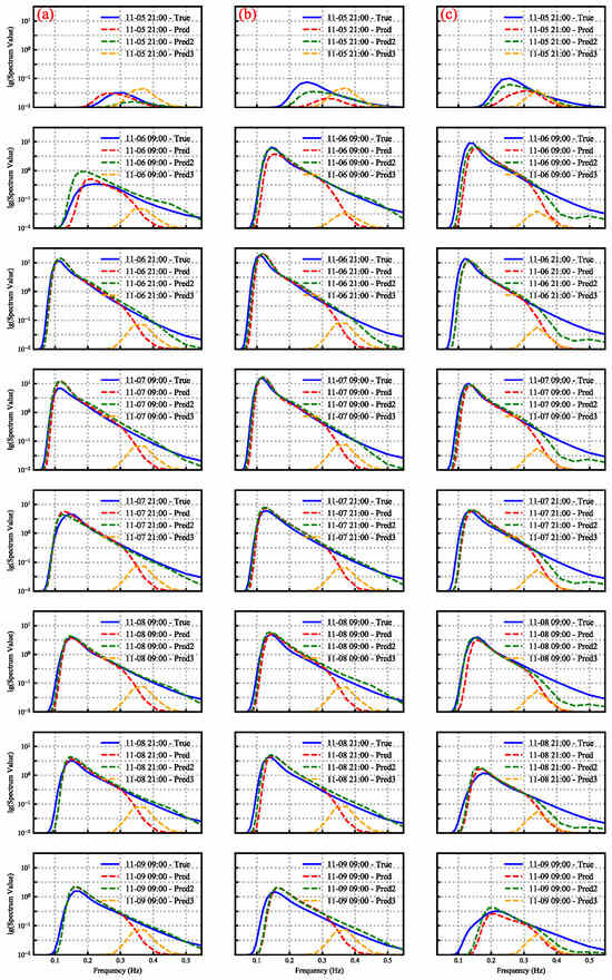
Figure 14.
Temporal evolution of wave spectra during the cold wave period with the Y-axis on a logarithmic scale (base 10), where (a) corresponds to point P1, (b) corresponds to point P2, and (c) corresponds to point P3.
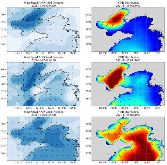
Figure 15.
Spatial distribution of wind speed and significant wave height in the area during the cold wave period.
Figure 14 shows that the wind-wave spectrum during the cold wave is unimodal with the main energy provided by the wave components corresponding to the narrow band frequencies. Starting from 09:00 on November 5th, the spectral energy at all three points is relatively low. From the 5th to the 6th, as the cold advection moves in, the wind speed strengthens, and the waves rapidly intensify. During the propagation of the spectrum from P3 to P1, processes such as wave breaking dissipation, nonlinear wave–wave interactions, and swell diffusion occur. Point P1, located near the coast, has a longer wave propagation path, so the growth of spectral energy is relatively delayed. The wave response at P2 and P3 is influenced by the lag of the wind field, resulting in overall lower energy levels. As the cold wave develops, the wind field gradually covers the entire Bohai Sea. Between the 6th and 7th, nonlinear interactions between wave components of different frequencies continuously transfer energy to lower frequencies, triggering the development of a low-frequency spectral peak. The spectral shape gradually changes from a broad peak to a narrow peak. The M0 first appears in Liaodong Bay and the central Bohai Sea, and by the 7th, it completely covers the Bohai Sea. Due to the transition from northeast winds to south winds, the wave propagation path also changes, with energy gradually transferring from the deep water region to the nearshore area. The model performs steadily during this phase and can capture the trend of the main frequency variation well. Between the 7th and 8th, the wave energy spreads to the Yellow Sea. As the wind field changes, the energy decreases, and the predicted values at the three points remain consistent with the real values. On the 8th and 9th, as the cold wave weakens and the wind direction shifts to northwest winds, the spectral energy generally decays. The offshore point P3 responds first with the spectral value decreasing. The energy dissipation curve from P3 to P2 to P1 is observed, but the spectral tail is still underestimated, which remains a key issue that needs to be addressed.
Therefore, we propose two methods to improve the predictive performance of the high-frequency part. One method is to strengthen the loss constraint on spectral values between 0.232 Hz and 0.548 Hz, guiding the model to pay more attention to high-frequency errors during the training process. The calculation method of the composite loss function is shown in Equation (29):
From Figure 14, it can be seen that the introduction of the high-frequency weighted loss function in the green curve significantly improves the spectral prediction performance of the model in the high-frequency frequency band. Most high-frequency spectral values are closer to the true values, indicating that this method can effectively guide the model to focus on the errors in the high-frequency part. However, there is still a certain deviation at point P3, which may be related to the short duration of the wind field at that point. Short-term wind drive is difficult to fully reflect the wave growth process, thereby affecting performance. Table 11 shows the comparison of prediction accuracy under different parameter settings. The results indicate that appropriate weighting can optimize the prediction performance, but parameters that are too large or too small can lead to an increase in error, indicating that a reasonable weighting amplitude is the key to improving model performance.
Table 11.
Comparison of predictive performance under different parameter combinations.
Throughout the entire process, as shown in Figure 15, the spatial distributions of wind speed and SWH demonstrate strong temporal and spatial consistency between the wind field and the wave field. The transformation of the spectral shape from a broad to a narrow peak, and the wave propagation path shifting from deep water to nearshore areas, both align with the advancing direction of the cold wave. The unique geographic structure of the Bohai Sea and surrounding areas restricts the full development of waves, resulting in the dominance of locally generated wind waves during the cold wave event. Changes in water depth and topography also influence wave propagation: waves intensify along the wind direction in deeper waters but attenuate as they approach the nearshore region due to increased bottom friction caused by shallower depths. This process reflects the physical characteristic that high-frequency components dissipate more easily, while low-frequency waves can propagate farther. Overall, the model successfully simulates the full process of wave generation, propagation, and attenuation, and it also verifies its ability to capture the spatial energy transfer patterns under a typical synoptic weather event.
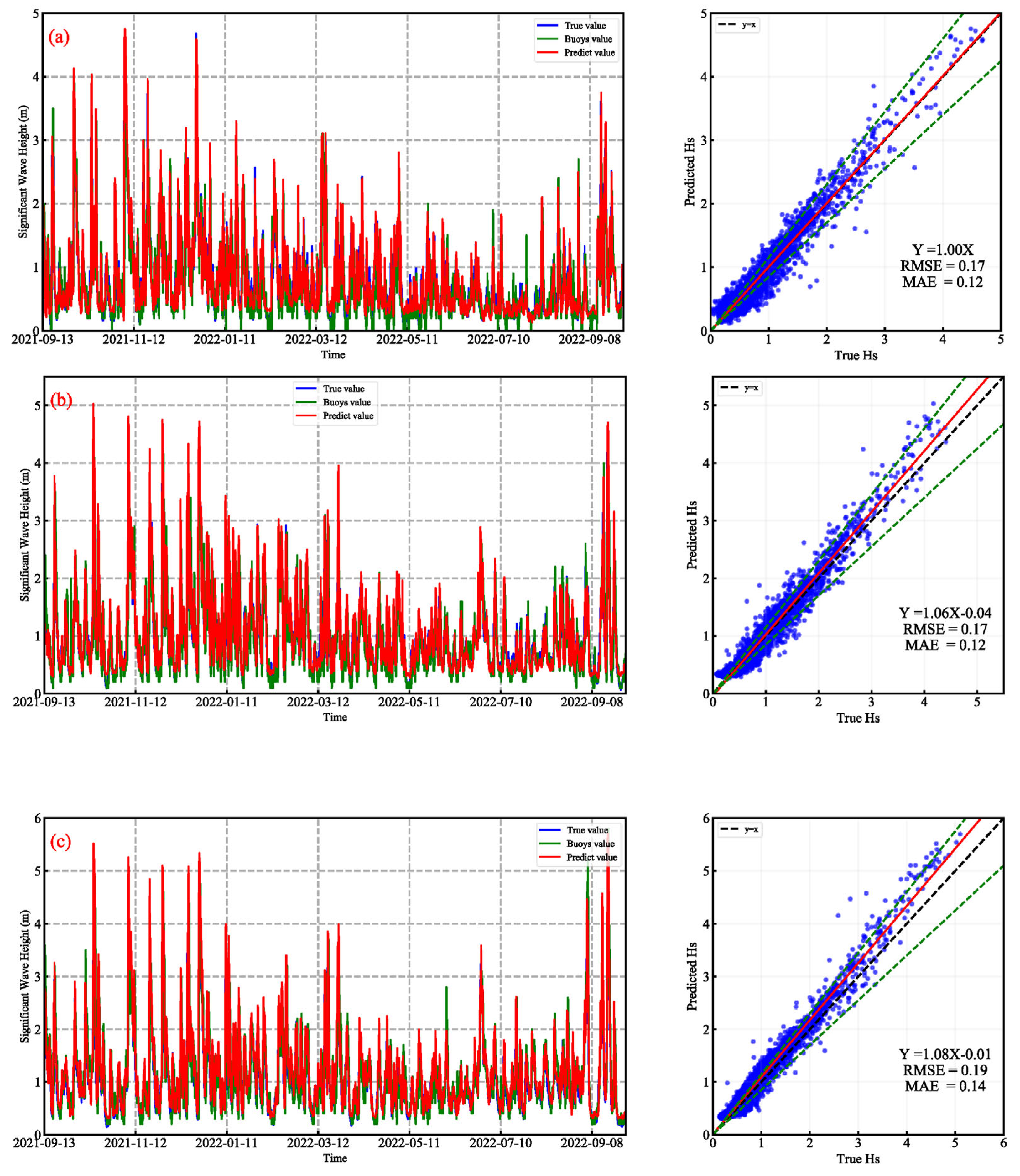
To further validate the model’s applicability under real observation conditions, buoy measurement data were introduced to compare the model’s predictions with ERA5 reanalysis data. In Figure 16, the blue line represents ERA5 reference values, the green line shows buoy observations, and the red line indicates model predictions. Subplots (a), (b), and (c) present the comparison of SWH predictions at representative points P2, P4, and P5. At point P2, the model predictions closely follow the overall trend of both ERA5 and buoy data, especially under regular wave conditions (SWH < 2.5 m), where the predicted curves closely align with the observed data. The scatter plot shows a high linear correlation between predictions and reference values with the regression line having a slope close to 1. At point P4, which is located in a semi-enclosed sea area, the linear regression equation is y = 1.06x − 0.04. Even for SWH between 2 m and 4 m, the model maintains good performance. At point P5, the model accurately captures SWH variations during most periods, remaining consistent with both ERA5 and buoy data. The overall error remains within an acceptable range, indicating the model’s ability to adapt to complex boundary conditions. In summary, the predictions at all three points are stable. Combined with the comparison against buoy observations, this further confirms the practical value and reliability of the proposed model.

Figure 16.
Time series comparison of SWH among predicted values, ERA5 reanalysis data, and buoy observations: (a) corresponds to point P2, (b) to point P4, and (c) to point P5.
4.3. Discussion
The results of this study demonstrate that the proposed method can effectively utilize deep learning models to achieve regional one-dimensional frequency spectrum prediction, showing strong practical applicability. In the spectrum regression task, one-dimensional spectra combined with various meteorological and oceanographic factors were used to reflect the spatiotemporal trends of spectral energy, thereby overcoming the limitations of traditional buoy observations in terms of spatial coverage and real-time capability. During the prediction process, we found that the model performed well in the dominant frequency band but showed systematic underestimation in the high-frequency range. This bias may stem from two main causes: first, deep learning models are generally biased toward fitting low-frequency signals while neglecting high-frequency components; second, in deep-sea regions, nonlinear interactions among waves transfer energy from the spectral peak to lower frequencies, which is a mechanism that the current model does not adequately capture. We attempted to improve the model’s ability to fit high-frequency spectral values by adding a high-frequency weighted loss function, and the results indicate that appropriate weighting can optimize the prediction performance. We also introduced Toba’s 3/2 exponential law [45,46] as a physical constraint, attempting to further standardize the model’s prediction results through the physical relationship of wind and wave growth. The calculation method of the loss function is shown in Equations (30) and (31):
In the equations, , , and . Considering that the value of is too small, it will affect the convergence speed of the model. Therefore, we set the condition that when is less than 0.1, will be set to 0, so that the overall loss function of the model only corresponds to the Smooth L1 loss function. At the same time, in order to ensure that the loss function is of the same magnitude, is 0.0001. From the orange curve in Figure 14, it can be seen that the results are very poor, possibly because the Toba 3/2 index rate may not be applicable to all sea conditions, especially in the presence of swells. In fact, the delayed response of wave fields to wind forcing plays a significant role in wave evolution, particularly during wind onset or under strong wind conditions. Improving the model’s ability to capture energy fluctuations during these periods will be our next focus. Compared to existing studies in the field, which mostly address either two-dimensional spectrum reconstruction or pointwise spectral prediction, our study achieves one-dimensional spectrum prediction at a regional scale, offering a distinct advantage.
Improvements made to the model during the deep learning training process have enhanced its overall stability, providing potential directions for future performance optimization. From a practical application perspective, although one-dimensional spectra can capture the evolution of wave energy in the frequency domain, they are limited in describing energy propagation and the directional dimension. Consequently, the model cannot capture critical processes such as directional spreading and energy focusing. Future research should consider using regional two-dimensional directional spectra to provide a more comprehensive representation of wave dynamics. These limitations highlight important directions for subsequent work.
5. Conclusions
This study investigates the problem of one-dimensional frequency spectrum prediction on a regional scale and proposes a hybrid network architecture combining CNN and xLSTM. We begin by analyzing physical variables to select input data that may influence prediction performance, thereby enhancing the model’s responsiveness to wind–wave dynamics. Based on the CNN-xLSTM framework, dropout and Layer Normalization are introduced, and the effect of pooling layers on feature extraction is considered. Residual connections are incorporated to retain key features. Extensive empirical evaluations over the Bohai and Yellow Seas demonstrate that the model exhibits strong generalization capability across various spatial scales and time points. In comparative experiments with mainstream CNN architectures, our model consistently outperforms others. Feature selection experiments reveal that incorporating water depth and mean sea-level pressure significantly reduces prediction error. When both variables are included, the RMSE of SWH reaches 0.138 m, and the MWP is 1.331 s, confirming the positive impact of input features on model performance. From a seasonal regional spectrum prediction perspective, the model effectively captures the spatial distribution of wave spectra at representative time points. In pointwise prediction analyses, most areas of the Bohai and Yellow Seas show good agreement in both spectral peak values and peak frequencies. To further assess the model’s capability in real-world large-scale weather scenarios, we analyze a typical cold wave event in November 2021. During this process, the model’s predicted spectra closely match the real spectra in terms of dominant frequency, energy magnitude, and spectral shape evolution. The model successfully tracks the trend of spectral energy changes at multiple locations: energy propagates from deep to shallow waters, high-frequency components dissipate more easily, and low-frequency waves travel farther—demonstrating the model’s timely responsiveness in complex meteorological environments. Moreover, applying a frequency-weighted loss function enhances the model’s ability to capture high-frequency spectral components, further improving prediction accuracy. A comparison with buoy-observed SWH shows that model predictions align well with both ERA5 data and buoy measurements, particularly for regular wave conditions (SWH < 2.5 m). Scatter plots indicate strong linear correlations, confirming the model’s practical reliability.
In conclusion, deep learning methods can effectively extract informative features from wave spectra and are suitable for regional-scale spectral forecasting. Moreover, integrating diverse input variables significantly enhances prediction accuracy. Although this study has certain limitations, these also point toward promising directions for future research.
Author Contributions
Conceptualization, W.H. and R.L.; Data curation, Y.L. and C.X.; methodology, Y.L.; software, Y.L.; validation, W.H., C.X. and P.R.; writing—original draft preparation, Y.L.; writing—review and editing, R.L.; funding acquisition, W.H. All authors have read and agreed to the published version of the manuscript.
Funding
This research was funded by the Key R&D Program of Shandong Province, China (No. 2024SFGC0201).
Data Availability Statement
The ERA5 data are available at the Climate Data Store (https://cds.climate.copernicus.eu/, accessed on 2 March 2025).
Acknowledgments
The authors would like to thank the Sea Marine Forecast and Hazard Mitigation Center of the Ministry of Natural Resources for providing assistance during the experiment.
Conflicts of Interest
The authors declare no conflicts of interest.
Appendix A
Wave element calculation formula
where
References
- Chen, C.; Sasa, K.; Prpić-Oršić, J.; Mizojiri, T. Statistical analysis of waves’ effects on ship navigation using high-resolution numerical wave simulation and shipboard measurements. Ocean Eng. 2021, 229, 108757. [Google Scholar] [CrossRef]
- Xu, F. Law of distribution of waves of disasters and disastrous waves in China. In Proceedings of the National Seminar on Disaster Reduction and Development in Coastal Areas, Yantai, China, 1–10 October 1991; p. 5. [Google Scholar]
- Powell, E.J.; Tyrrell, M.C.; Milliken, A.; Tirpak, J.M.; Staudinger, M.D. A review of coastal management approaches to support the integration of ecological and human community planning for climate change. J. Coast. Conserv. 2019, 23, 1–18. [Google Scholar] [CrossRef]
- Qiu, S.; Liu, K.; Wang, D.; Ye, J.; Liang, F. A comprehensive review of ocean wave energy research and development in China. Renew. Sustain. Energy Rev. 2019, 113, 109271. [Google Scholar] [CrossRef]
- Oliveira-Pinto, S.; Rosa-Santos, P.; Taveira-Pinto, F. Electricity supply to offshore oil and gas platforms from renewable ocean wave energy: Overview and case study analysis. Energy Convers. Manag. 2019, 186, 556–569. [Google Scholar] [CrossRef]
- Wen, S. Wave Theory and Calculation Principle; Science Press: Beijing, China, 1984. [Google Scholar]
- Pierson, W.J., Jr.; Moskowitz, L. A proposed spectral form for fully developed wind seas based on the similarity theory of S. A. Kitaigorodskii. J. Geophys. Res. 1964, 69, 5181–5190. [Google Scholar] [CrossRef]
- Tolman, H.L. A Third-Generation Model for Wind Waves on Slowly Varying, Unsteady, and Inhomogeneous Depths and Currents. J. Phys. Oceanogr. 1991, 21, 782–797. [Google Scholar] [CrossRef]
- Tolman, H.L.; Chalikov, D. Source terms in a third-generation wind wave model. J. Phys. Oceanogr. 1996, 26, 2497–2518. [Google Scholar] [CrossRef]
- Luo, Q.-R.; Xu, H.; Bai, L.-H. Prediction of significant wave height in hurricane area of the Atlantic Ocean using the Bi-LSTM with attention model. Ocean Eng. 2022, 266, 112747. [Google Scholar] [CrossRef]
- Bethel, B.J.; Sun, W.; Dong, C.; Wang, D. Forecasting hurricane-forced significant wave heights using a long short-term memory network in the Caribbean Sea. Ocean Sci. 2022, 18, 419–436. [Google Scholar] [CrossRef]
- Pushpam, M.M.P.; Enigo, F. Forecasting Significant Wave Height using RNN-LSTM Models. In Proceedings of the 2020 4th International Conference on Intelligent Computing and Control Systems (ICICCS), Madurai, India, 13–15 May 2020; pp. 1141–1146. [Google Scholar]
- Minuzzi, F.C.; Farina, L. A deep learning approach to predict significant wave height using long short-term memory. Ocean Model. 2023, 181, 102151. [Google Scholar] [CrossRef]
- Wang, L.; Deng, X.; Ge, P.; Dong, C.; Bethel, B.; Yang, L.; Xia, J. CNN-BiLSTM-Attention Model in Forecasting Wave Height over South-East China Seas. Comput. Mater. Contin. 2022, 73, 2151–2168. [Google Scholar] [CrossRef]
- Krizhevsky, A.; Sutskever, I.; Hinton, G.E. ImageNet classification with deep convolutional neural networks. Commun. ACM 2017, 60, 84–90. [Google Scholar] [CrossRef]
- Bai, G.; Wang, Z.; Zhu, X.; Feng, Y. Development of a 2-D deep learning regional wave field forecast model based on convolutional neural network and the application in South China Sea. Appl. Ocean Res. 2022, 118, 103012. [Google Scholar] [CrossRef]
- Zhou, S.; Xie, W.; Lu, Y.; Wang, Y.; Zhou, Y.; Hui, N.; Dong, C. ConvLSTM-Based Wave Forecasts in the South and East China Seas. Front. Mar. Sci. 2021, 8, 680079. [Google Scholar] [CrossRef]
- Beck, M.; Pöppel, K.; Spanring, M.; Auer, A.; Prudnikova, O.; Kopp, M.; Klambauer, G.; Brandstetter, J.; Hochreiter, S. xlstm: Extended long short-term memory. arXiv 2024, arXiv:2405.04517. [Google Scholar]
- Zeng, X.; Qi, L.; Yi, T.; Liu, T. A Sequence-to-Sequence Model Based on Attention Mechanism for Wave Spectrum Prediction. In Proceedings of the 2020 11th International Conference on Awareness Science and Technology (iCAST), Qingdao, China, 7–9 December 2020; pp. 1–5. [Google Scholar]
- Liu, S.; Zhang, X. A Wave Prediction Framework Based on Machine Learning and the Third Generation Wave Model. J. Offshore Mech. Arct. Eng. 2021, 144, 011202. [Google Scholar] [CrossRef]
- Hasselmann, K.; Barnett, T.P.; Bouws, E.; Carlson, H.; Cartwright, D.E.; Enke, K.; Ewing, J.A.; Gienapp, A.; Hasselmann, D.E.; Kruseman, P.; et al. Measurements of wind-wave growth and swell decay during the joint North Sea wave project (JONSWAP). Ergaenzungsheft Zur Dtsch. Hydrogr. Z. Reihe A 1973, 12. [Google Scholar]
- Jiang, H. Wind speed and direction estimation from wave spectra using deep learning. Atmos. Meas. Tech. 2022, 15, 1–9. [Google Scholar] [CrossRef]
- Song, Y.; Jiang, H. A Deep Learning–Based Approach for Empirical Modeling of Single-Point Wave Spectra in Open Oceans. J. Phys. Oceanogr. 2023, 53, 2089–2103. [Google Scholar] [CrossRef]
- Hersbach, H.; Bell, B.; Berrisford, P.; Hirahara, S.; Horányi, A.; Muñoz-Sabater, J.; Nicolas, J.; Peubey, C.; Radu, R.; Schepers, D.; et al. The ERA5 global reanalysis. Q. J. R. Meteorol. Soc. 2020, 146, 1999–2049. [Google Scholar] [CrossRef]
- Hasan, S.H.; Hasan, S.H.; Ahmed, M.S.; Hasan, S.H. A Novel Cryptocurrency Prediction Method Using Optimum CNN. Comput. Mater. Contin. 2022, 71, 1051–1063. [Google Scholar] [CrossRef]
- Choi, H.; Park, M.; Son, G.; Jeong, J.; Park, J.; Mo, K.; Kang, P. Real-time significant wave height estimation from raw ocean images based on 2D and 3D deep neural networks. Ocean Eng. 2020, 201, 107129. [Google Scholar] [CrossRef]
- Liu, S.; Zhang, C.; Ma, J. CNN-LSTM Neural Network Model for Quantitative Strategy Analysis in Stock Markets. In Proceedings of the Neural Information Processing, Guangzhou, China, 14–18 November 2017; pp. 198–206. [Google Scholar]
- Greff, K.; Srivastava, R.K.; Koutník, J.; Steunebrink, B.R.; Schmidhuber, J. LSTM: A search space odyssey IEEE Trans. Neural Netw. Learn. Syst. 2016, 28, 2222–2232. [Google Scholar] [CrossRef] [PubMed]
- Milakov, M.; Gimelshein, N. Online normalizer calculation for softmax. arXiv 2018, arXiv:1805.02867. [Google Scholar] [CrossRef]
- Kohonen, T. Correlation Matrix Memories. IEEE Trans. Comput. 1972, C-21, 353–359. [Google Scholar] [CrossRef]
- Anderson, J.A. A simple neural network generating an interactive memory. Math. Biosci. 1972, 14, 197–220. [Google Scholar] [CrossRef]
- Nakano, K. Associatron-A Model of Associative Memory. IEEE Trans. Syst. Man Cybern. 1972, SMC-2, 380–388. [Google Scholar] [CrossRef]
- Sejnowski, T.J. Storing covariance with nonlinearly interacting neurons. J. Math. Biol. 1977, 4, 303–321. [Google Scholar] [CrossRef]
- Dayan, P.; Willshaw, D.J. Optimising synaptic learning rules in linear associative memories. Biol. Cybern. 1991, 65, 253–265. [Google Scholar] [CrossRef]
- Ioffe, S.; Szegedy, C. Batch Normalization: Accelerating Deep Network Training by Reducing Internal Covariate Shift. In Proceedings of the 32nd International Conference on Machine Learning, Lille, France, 7–9 July 2015; pp. 448–456. [Google Scholar]
- Ba, J.L.; Kiros, J.R.; Hinton, G.E. Layer normalization. arXiv 2016, arXiv:1607.06450. [Google Scholar]
- Cavaleri, L.; Abdalla, S.; Benetazzo, A.; Bertotti, L.; Bidlot, J.R.; Breivik, Ø.; Carniel, S.; Jensen, R.E.; Portilla-Yandun, J.; Rogers, W.E.; et al. Wave modelling in coastal and inner seas. Prog. Oceanogr. 2018, 167, 164–233. [Google Scholar] [CrossRef]
- Xu, W.; Li, R.; Hu, W.; Cui, W.; Xu, C.; Wang, N. Study on the Construction and training method of wave height field prediction model for the Bohai and Yellow Seas based on convolutional neural network. Mar. Sci. Bull. 2025, 44, 1–14. [Google Scholar]
- Wang, J.; Li, B.; Gao, Z.; Wang, J. Comparison of ECMWF Significant Wave Height Forecasts in the China Sea with Buoy Data. Weather Forecast. 2019, 34, 1693–1704. [Google Scholar] [CrossRef]
- Bidlot, J.-R. Twenty-one years of wave forecast verification. ECMWF Newsl. 2017, 150, 31–36. [Google Scholar]
- Perrie, W.; Toulany, B.; Casey, M. A Generalized Two–Scale Approximation for Ocean Wave Models. Front. Mar. Sci. 2022, 9, 867423. [Google Scholar] [CrossRef]
- Csanady, G.; Lumley, J. Air-Sea Interaction: Laws and Mechanisms; Cambridge University Press: Cambridge, UK, 2002; Volume 55, p. B117. [Google Scholar]
- Rahaman, N.; Baratin, A.; Arpit, D.; Draxler, F.; Lin, M.; Hamprecht, F.; Bengio, Y.; Courville, A. On the Spectral Bias of Neural Networks. In Proceedings of the 36th International Conference on Machine Learning, Long Beach, CA, USA, 9–15 June 2019; pp. 5301–5310. [Google Scholar]
- Meng, Q.Z.; Luo, Q.; Yang, K.; Ren, H.; Gong, Y. Causes of the Extreme Rain and Snow in Northern China in Early November 2021. Desert Oasis Meteorol. 2022, 1–10. [Google Scholar]
- Guan, C.; Xie, L. On the linear parameterization of drag coefficient over sea surface. J. Phys. Oceanogr. 2004, 34, 2847–2851. [Google Scholar] [CrossRef]
- Toba, Y. Local balance in the air-sea boundary processes: I. On the growth process of wind waves. J. Oceanogr. 1972, 28, 109–120. [Google Scholar] [CrossRef]


Disclaimer/Publisher’s Note: The statements, opinions and data contained in all publications are solely those of the individual author(s) and contributor(s) and not of MDPI and/or the editor(s). MDPI and/or the editor(s) disclaim responsibility for any injury to people or property resulting from any ideas, methods, instructions or products referred to in the content. |
© 2025 by the authors. Licensee MDPI, Basel, Switzerland. This article is an open access article distributed under the terms and conditions of the Creative Commons Attribution (CC BY) license (https://creativecommons.org/licenses/by/4.0/).