A Channel-Aware AUV-Aided Data Collection Scheme Based on Deep Reinforcement Learning

Abstract

Underwater sensor networks (UWSNs) play a crucial role in subsea operations like marine exploration and environmental monitoring. A major challenge for UWSNs is achieving effective and energy-efficient data collection, particularly in deep-sea mining, where energy limitations and long-term deployment are key concerns. This study introduces a Channel-Aware AUV-Aided Data Collection Scheme (CADC) that utilizes deep reinforcement learning (DRL) to improve data collection efficiency. It features an innovative underwater node traversal algorithm that accounts for unique underwater signal propagation characteristics, along with a DRL-based path planning approach to mitigate propagation losses and enhance data energy efficiency. CADC achieves a 71.2% increase in energy efficiency compared to existing clustering methods and shows a 0.08% improvement over the Deep Deterministic Policy Gradient (DDPG), with a 2.3% faster convergence than the Twin Delayed DDPG (TD3), and reduces energy cost to only 22.2% of that required by the TSP-based baseline. By combining a channel-aware traversal with adaptive DRL navigation, CADC effectively optimizes data collection and energy consumption in underwater environments.

1. Introduction

The vastness and complexity of the ocean generate substantial volumes of diverse marine data, particularly in emerging fields such as deep-sea mining. Underwater Wireless Sensor Networks (UWSNs) are integral to the communication infrastructure necessary for deep-sea equipment, being as effective data collection facilitates precise monitoring of sediment plumes, equipment status, and environmental parameters, all of which are essential to ensure safe mining operations. Unlike terrestrial applications, the focus in these underwater environments is on energy efficiency rather than real-time performance, with daily data transmissions deemed sufficient for operational needs [1,2].

Deep-sea mining environments introduce unique challenges for underwater sensor networks. At depths exceeding 5000 m, the network nodes encounter significant energy constraints and face considerable maintenance difficulties while collecting vital parameters such as suspended particle concentrations, turbidity, and bioacoustic signals. Consequently, data collection methods must adeptly balance three core demands: maximizing net work–lifespan through energy optimization, ensuring reliable data delivery in challenging acoustic channels, and maintaining operational stability for multi-year deployments. These requirements underscore the urgent need for innovative data collection paradigms that go beyond traditional real-time transmission methods [3].

The importance of underwater network data collection lies in its foundational role for deep-sea operations. These sensor nodes serve as the “eyes” and “ears” for mining activities, generating multi-dimensional data streams that include sediment dispersion patterns, equipment vibration signatures, and biological acoustic profiles [1]. The quality and continuity of these data streams are crucial for (1) accurately mapping resource distribution; (2) swiftly addressing equipment anomalies; and (3) conducting environmental impact assessments necessary for sustainable mining practices [4].

The extreme deep-sea environment is characterized by three predominant factors: ultra-high pressure, salinity gradient stratification, and severe signal refraction, scattering, attenuation and temporal–spatial uncertainty. Collectively, these factors induce highly time-varying asymmetric characteristics in underwater acoustic channels, resulting in exponential growth in signal propagation loss, which is manifested as path attenuation and multipath effects [5]. Consequently, this scenario leads to a significant degradation of both packet error rate (PER) and bit error rate (BER).

Underwater data collection methods can be categorized into three main types: stationary, mobile, and hybrid. The stationary method involves a network of underwater sensor nodes that relay data to the surface [6,7]. This approach incurs significant energy costs due to battery limitations, leading to conflicts between high energy consumption and reduced operational lifespan. The mobile method utilizes Autonomous Underwater Vehicles (AUVs), which can travel to underwater points of interest as needed. This approach is flexible and suitable for urgent surveys but is limited by space for scientific instruments and cannot support long-term monitoring. The hybrid method combines stationary sensors with AUVs. In this setup, sensors conduct long-term surveillance while AUVs relay data to the surface. This direct single-hop communication reduces energy expenditure per node and extends net work–lifespan by minimizing multi-hop forwarding energy [4,8].

As a result, the hybrid approach has emerged as a pivotal strategy for enhancing underwater data collection, showing significant promise in reducing network energy consumption and extending operational longevity. However, realizing these benefits depends on the implementation of advanced path planning strategies that optimize trajectory efficiency while ensuring the reliability of acoustic links. Current AUV path planning algorithms primarily depend on simplistic Euclidean distance metrics for trajectory determination, while existing methods attempt to reduce energy consumption by focusing on proximity to target nodes. This basic strategy inadequately tackles the complexities of underwater acoustic propagation loss.

Traditional path planning for AUVs using node proximity strategies can result in high packet loss due to asymmetric acoustic channel characteristics in underwater environments. To enhance long-distance data collection, sensor nodes often increase transmission power to counteract acoustic propagation loss, which reduces the network’s lifespan. Therefore, integrating an acoustic propagation model into the path planning framework is essential for optimizing data collection in AUV-assisted networks.

In this paper, we leverage the state-of-the-art acoustic propagation model and fully consider the realistic signal propagation characteristics of the underwater channel. Specifically, we present a channel-aware data acquisition strategy for AUVs, which pre-calculates the regions with low propagation loss of acoustic signals based on the underwater signal model. Additionally, the proposed method employs reinforcement learning algorithms to dynamically plan the AUV’s path, thereby circumventing areas of high loss. This approach aims to enhance the energy efficiency associated with underwater data acquisition. The main contributions are as follows.

• This study pioneers a channel-aware node traversal algorithm for AUVs, optimizing energy efficiency and data collection rates by integrating asymmetric acoustic propagation characteristics with signal strength analysis, moving beyond traditional distance-only metrics.
• In response to the challenges of underwater data collection, we propose an AUV-aided path planning algorithm based on DRL. This algorithm takes into account key factors such as underwater propagation loss, underwater obstacles, and ocean currents to achieve efficient data collection rates and energy consumption optimization.
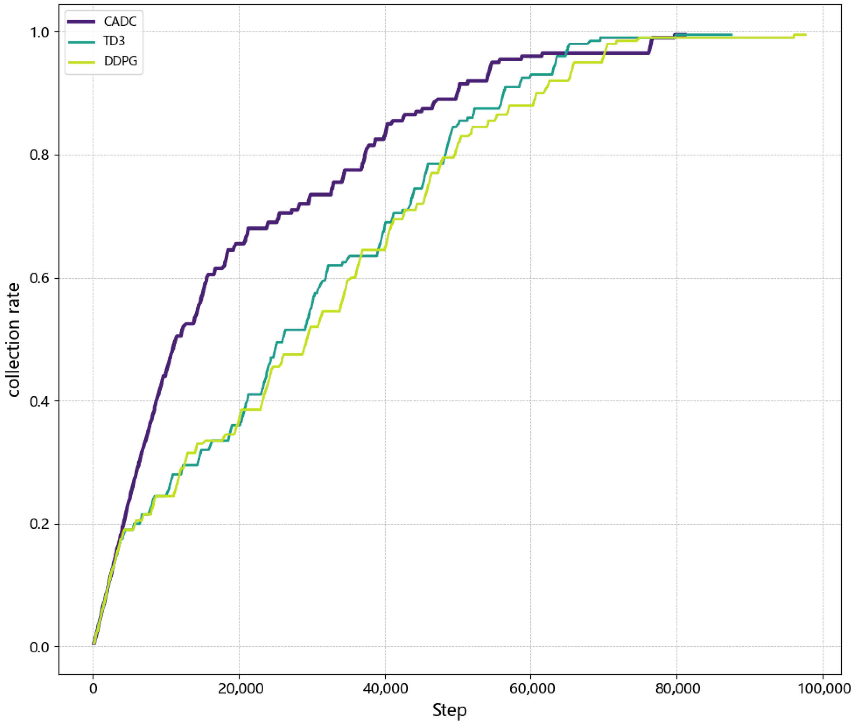
• Extensive simulations demonstrate that the proposed algorithm achieves a 71.2% improvement in energy efficiency compared to clustering-based methods and a 2.3% faster convergence than TD3, validating its capability to optimize AUV paths through asymmetric channel-aware trajectory planning while minimizing network energy consumption.

The remainder of this paper is organized as follows. Section 2 briefly reviews the related works regarding the underwater data collection problem. Section 3 describes the network architecture, underwater acoustic channel model, energy consumption model, and optimization objective. Section 4 introduces two main components of the algorithm: a task allocation algorithm that fully considers the unique propagation characteristics of the underwater environment, and a path planning algorithm based on reinforcement learning. Section 5 validates the effectiveness of the algorithm through simulations. Section 6 presents the conclusion of the algorithm.

2. Related Works

Current underwater data collection methods can be categorized into three main groups: data collection methods which rely on UWSN, AUV-based data collection methods, and combined UWSN and AUV-assisted methods.

2.1. Data Collection Methods Relying on UWSN

In utilizing UWSN for data collection, well-designed routing protocols are crucial, and they can optimize the routing between source and destination nodes based on specific application scenarios. For example, the ACARP protocol proposes an adaptive channel-aware routing protocol for large-scale UWSN environments that is capable of actively sensing channel changes among nodes [7]. Guo et al. proposes an adaptive routing protocol for underwater delay/disruption-tolerant sensor networks [9]. The CARMA protocol designs a multi-path adaptive routing strategy for UWSN based on channel-aware reinforcement learning, which aims to maximize the packet delivery rate and minimize energy consumption by jointly determining the capacity and composition of packet relay sets [10]. Nevertheless, the data collection scheme for multi-hop transmission is more suitable for urgent or high-value data transmission. When facing the demand of large amounts of data transmission, the limited power of UWSN nodes may be difficult to meet the long-term application requirements [11].

2.2. AUV-Based Data Collection Methods

The use of AUV-assisted data collection can greatly extend the lifetime of UWSN nodes, especially when network nodes store a large amount of routinely data. There are various categories into which common AUV data collection algorithms can be classified: 1. clustering-based data collection schemes, 2. data collection schemes based on the information value of the data, and 3. data collection schemes using reinforcement learning algorithms [11].

2.2.1. Clustering-Based Data Collection Schemes

Several research works use the algorithm that employs clustering [8,12,13]. Intra-cluster nodes send data to cluster heads; subsequently, AUVs collect the data stored in these cluster heads through path planning. In [8], the path planning of an AUV is optimized to maximize value of information (VoI) of data collection. Jiang et al. propose a data collection framework supported by AUVs, utilizing the Hybrid Clustering and Matrix Completion (AHMC) methodology, to enhance data collection efficiency [8]. A clustering algorithm is proposed in [12] to reduce the latency and energy consumption of data collection by optimizing cluster formation and path planning for AUVs. A multi-AUV collaborative data collection scheme, which includes clustering and routing strategies, is presented in [13]. Through the collaboration of multiple AUVs, the efficiency of data collection and the coverage of the network are improved.

2.2.2. Data Collection Schemes Based on the Information Value of the Data

In [14], the authors propose a hierarchical collection strategy based on the VoI. AUV-aided transmission and multi-hop transmission are utilized to determine the trade-off between energy consumption and network performance based on the VoI in a cluster. By developing an analytic expression for VoI attenuation and employing multi-hop routing and AUVs for data transmission, a hybrid data collection scheme (HDCS) tackles real-time data collection and energy efficiency challenges [15]. To ensure the maximization of the VoI within a given time, a dynamic value-based path planning strategy is designed for the AUV, enabling it to dynamically visit data collectors [16].

2.2.3. Reinforcement Learning-Based Data Collection Schemes

In order to enable successful data collection, refs. [11,17,18,19] use reinforcement learning algorithms to plan the AUV’s travel path. Ref. [11] proposes a collaborative ocean data collection method for multi autonomous underwater robots (AUVs) based on localized global deep Q-network (LG-DQN) and data value. A multi-AUV-assisted data collection framework based on offline reinforcement learning, which optimizes data transmission rate, information value, and energy consumption while ensuring collision avoidance, is proposed in [17]. A digital pheromone and target uncertainty map based data collection scheme for the AUV swarm in a cooperative and secure manner is proposed in [18]. A DQN-based learning algorithm to determine the optimal strategy is developed in [19]. Beyond path planning, recent advances apply DRL to optimize physical-layer communication resources in UWSN. These techniques address channel dynamics through adaptive modulation and coding (AMC), complementing network-layer path optimization. The AMUSE framework [20] pioneers the use of Multi-Armed Bandits (MABs) for adaptive modulation selection. By avoiding computationally intensive deep learning, it achieves 80.65% energy savings while maintaining reliability—particularly suited for resource-constrained nodes. However, its focus on modulation alone limits adaptability in highly dynamic channels. Building upon lightweight foundations, subsequent research introduced predictive capabilities to handle turbulent underwater channels. The integration of LSTM-based channel prediction with reinforcement learning enables real-time adaptation to rapid environmental changes, overcoming the limitation of outdated channel state information. This hybrid approach demonstrates 23% throughput improvement under bit error rate constraints [21]. The evolution culminates in joint optimization schemes that simultaneously address modulation, coding, and quality-of-service requirements. Validated through rigorous pool and sea trials, these integrated solutions achieve a 44% BER reduction alongside 25% energy savings—representing the current state of the art in physical-layer adaptation [22].

2.3. Combined UWSN and AUV-Assisted Methods

In delay-sensitive and energy-efficient applications, it is necessary to use a UWSN combined with AUV-assisted data collection methods [11,13,23]. Data are categorized into urgent and non-urgent types in [11], with the non-urgent data further divided into high-value and low-value data. By leveraging the collaboration between underwater acoustic networks and AUVs for data collection, it meets the timeliness requirements of various data types. An integrated approach that optimizes clustering and path planning holistically is proposed in [13], providing a comprehensive and balanced solution for multi-AUV collaborative data collection. By balancing network energy consumption and data collection latency, the method aims to integrate data gathering by multi-hop transmission and data gathering by AUVs. The challenge of ascertaining data importance levels without relying on domain-specific knowledge is addressed in [23], and delay time requirements are established based on their significance. Subsequently, it employs an integrated approach for collecting sensing data in UWSN, combining multi-hop transmission with data gathering by AUVs.

3. System Model

3.1. Network Architecture

We are considering a scenario of data collection by a single AUV, as illustrated in Figure 1. It consists of N fixed sensor nodes (SNs) positioned in three-dimensional space, and one AUV. SNs are randomly deployed in $L\times W\times H$ space, and their static locations can be obtained through localization algorithms [24].

AUV is responsible for collecting data from these nodes, thereby avoiding the extensive transmission of routine data that could deplete the nodes’ energy reserves prematurely. During the motion of AUV, the impact of ocean currents is not negligible. In our model, we have specifically focused on the potential influence of ocean currents along the x-axis and y-axis on the AUV’s movement, as highlighted in previous research [25].

3.2. Underwater Acoustic Channel Model

Underwater acoustic channel is considered one of the most complex propagation channels [26]. Propagation loss and ocean background noise are the two main factors affecting the reliable data reception at the receiver [27].

The transmission loss ($TL$) of underwater acoustic waves is a complex process shaped by the interplay of various factors, which together determine the characteristics of sound transmission through the aquatic medium [28]. The speed of sound fluctuates with variations in water depth, temperature, and salinity. As sound waves travel, they are subject to signal attenuation due to absorption and scattering, and the phenomenon of multi-path propagation is prevalent, with signals reaching the receiver via multiple pathways [29]. A thorough understanding of these characteristics is essential for the design and optimization of underwater communication systems and acoustic sensors.

Figure 2 illustrates $TL$ of nodes at various depths. It is evident that the data sent by the source node experience loss and undergo reflection and refraction in the underwater space. The AUV needs to plan its path based on these propagation characteristics to better communicate with underwater nodes. Next, we illustrate the uniqueness of the underwater acoustic channel by examining its propagation characteristics at four different depths:

(1)

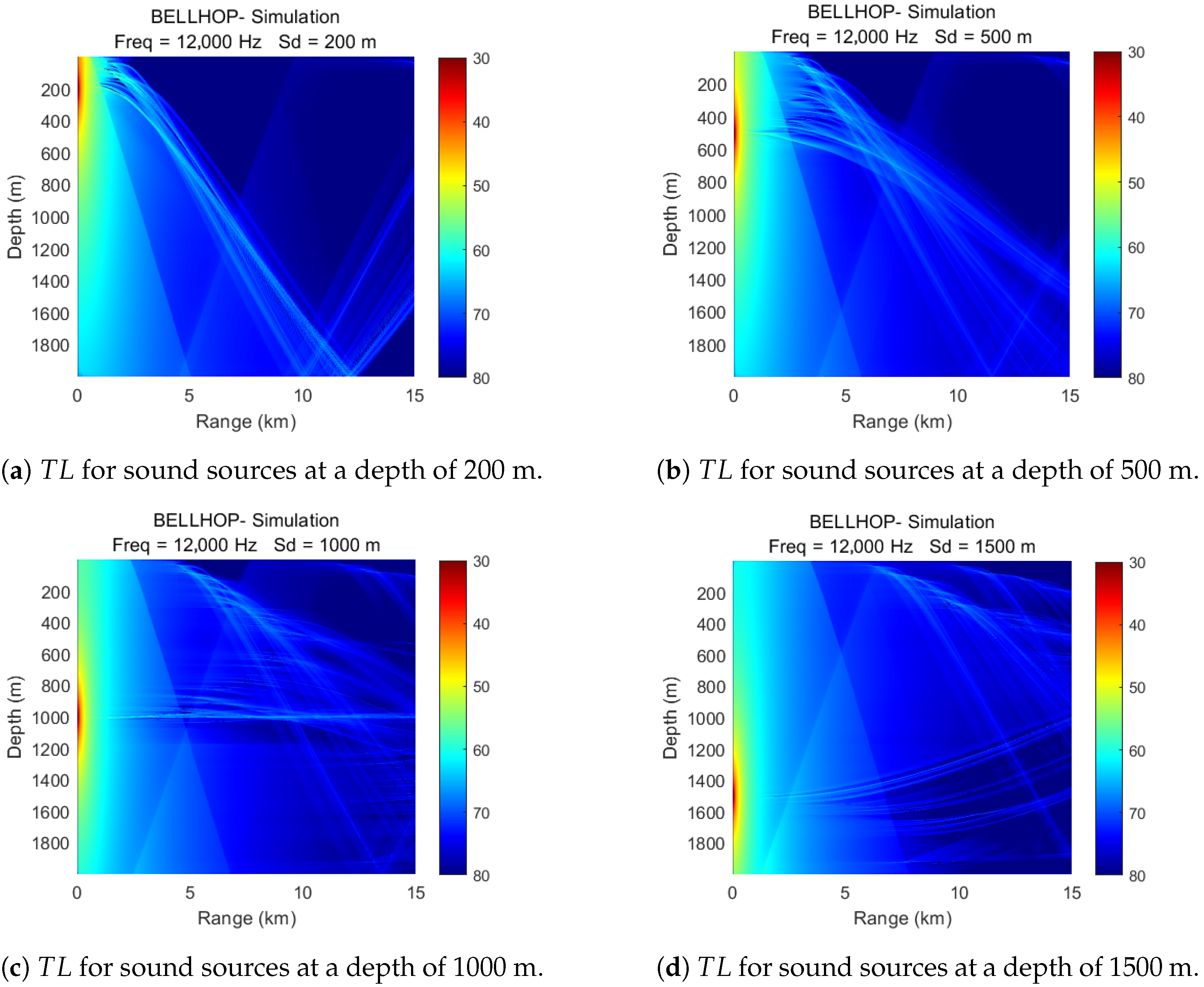
In Figure 2a, it is clearly observed that there are large shaded areas in the propagation loss and when the AUV is located in these areas, communication with the nodes will become difficult. At the same time, the clear and bright curves show that communication is still possible despite the longer distance between the AUV and the node.

(2)

Source node located at 500 m in Figure 2b shows similar characteristics in terms of $TL$ as at 200 m, although the shaded area is reduced and the clear and bright curves in the figure cover a wider area. As a result, the active area available for AUV selection increases accordingly.

(3)

As the depth of the node drops to 1000 m as in Figure 2c, a distinct acoustic channel axis develops, which is the most significant difference from the propagation loss characteristics of shallower depth source nodes. An AUV at a water depth of approximately 1000 m still has a high probability of communicating with the source node even if it is far away from it.

(4)

As shown in Figure 2d, when the node is located at a water depth of 1500 m, the shadow zone is mainly concentrated in the area that is deeper and farther away from the source node. At the same time, the sound reflection phenomenon near the water surface is quite obvious.

Figure 2. $TL$ at different sound source depths.

Figure 2. $TL$ at different sound source depths.

In order to improve the success rate of data collection, the conventional practices are to keep AUV close enough to the nodes, cluster heads, or specific key nodes before data collection. This practice, while ensuring a low BER, often leads to a non-optimal optimization objective. When we fully consider the special propagation characteristics, AUVs must fully take these characteristics into account during path planning. For example, when collecting data from the node in Figure 2c, which is located at a water depth of 1000 m, the AUV can choose a location close to the node, or travel to the acoustic channel axis to collect the data, or motor to an area close to the water surface where $TL$ is lower.

Furthermore, environmental noise from marine life activities, shipping traffic, and natural occurrences adds an extra layer of complexity to signal detection and the reliability of communication [30]. The total underwater noise $N\left(f\right)$ [27] can be expressed as follows:

$$N\left(f\right)=N_t\left(f\right)+N_s\left(f\right)+N_w\left(f\right)+N_{th}\left(f\right).$$

(1)

where $N_t\left(f\right)$, $N_s\left(f\right)$, $N_w\left(f\right)$, and $N_{th}\left(f\right)$ represent the turbulence noise, shipping noise, wave noise and thermal noise, respectively. The description of these noises [31] is stated as

$$\begin{array}{c}10log{N}_t\left(f\right)=17-30logf,\hfill \\ 10log{N}_s\left(f\right)=40+20(s-0.5)+26logf-60(f+0.03),\hfill \\ 10log{N}_w\left(f\right)=50+7.5w^{0.5}+20logf-40log(f+0.4),\hfill \\ 10log{N}_{th}\left(f\right)=-15+20logf.\hfill \end{array}$$

(2)

where f represents the frequency [kHz] of the signal.

The signal-to-noise ratio ($SNR$) at the receiver must satisfy the following formula:

$$SNR=SL-TL-10logN\left(f\right)+DI.$$

(3)

where the $SNR$ must meet the minimum threshold requirement. The source level $SL$ can be calculated as (4) [27,31]; the directivity index $DI$ [31] is set to 0 dB.

$$SL=10log{P}_t+171.$$

(4)

where $P_t$ represents the transmit power.

The PER $p_{PER}$ is calculated based on the BER [32]. There are no bit errors only if all bits are received correctly. The formula for calculating the PER is as follows:

$$p_{PER}=1-{(1-P_{BER})}^n.$$

(5)

where the BER is represented by $P_{BER}$, which is calculated based on the $SNR$ and modulation method [32,33]. For OFDM systems employing BPSK modulation, the BER in an additive white gaussian noise (AWGN) channel is approximated as follows [34]:

$$p_{BER}=Q\left(\sqrt{2\times SNR}\right).$$

(6)

3.3. Ocean Currents Model

Ocean currents, as a key environmental factor affecting AUV path planning, have a vector superposition effect on AUV speed, enabling a more realistic simulation of the underwater environment. Ocean currents at different locations have different directions and intensities. Ocean currents have a significant impact on the performance of AUVs, and AUVs need to frequently adjust their heading to maintain their posture. In practical applications, we can use the Navier–Stokes equations to model the ocean current flow field by simulating multiple single point vortices, namely the superposition of viscous Lamb vortices [35]. This method can help us obtain information on the direction and magnitude of ocean currents. The mathematical expression for a single Lamb vortex is shown below:

$$v_x^n\left(p\right)=-\Gamma {\displaystyle \frac{y-y_{center}}{2\pi {\left(p-p_{center}\right)}^2}}\left[1-e^{-\left({\displaystyle \frac{{\left(p-p_{center}\right)}^2}{{\delta }^2}}\right)}\right]$$

(7)

$$v_y^n\left(p\right)=\Gamma {\displaystyle \frac{x-x_{center}}{2\pi {\left(p-p_{center}\right)}^2}}\left[1-e^{-\left({\displaystyle \frac{\left(p-p_{center}\right.}{{\delta }^2}}\right)}\right]$$

(8)

$$\omega \left(p\right)={\displaystyle \frac{\Gamma }{\pi {\delta }^2}}{e}^{-\left({\displaystyle \frac{{\left(p-p_{center}\right)}^2}{{\delta }^2}}\right)}$$

(9)

where $p_{center}$ represents the position of the vortex center, $\delta$ denotes the vortex radius, $\Gamma$ indicates the intensity of the vortex, $\omega \left(p\right)$ signifies the vorticity of the vortex, and p denotes the position vector of the AUV.

3.4. Energy Optimization Model and Problem Formulation

In the network, the sensor nodes are significantly more difficult to recharge than the AUVs, which can be powered up by surfacing to the water surface or utilizing a charging base station. Therefore, we consider an optimization objective that includes not only maximizing the total amount of data collected but also minimizing the energy consumption of the entire network. The energy cost ($EC$) can be estimated as the ratio of the total energy consumption to the total collected data:

$$EC={\displaystyle \frac{{\sum }_i^N{E}_{n_i}+\sum E_{auv}}{{\sum }_i^N{C}_i}}(\mathrm{Unit}:\mathrm{J}/\mathrm{byte})$$

(10)

where ${\sum }_i^N{E}_{n_i}$ denotes the total energy consumption (in joules, J) of the nodes during the period in which the AUV collects data from the network. $\sum E_{auv}$ is the energy consumption associated with AUV movement, calculated as $\sum E_{auv}={\sum }_{t=1}{P}_t^{motion}\times \Delta t$. $C_i$ represents the total amount of data collected by the AUV from node i (in bytes).

In order to maximize the benefits, the optimization objective is to minimize the energy consumption required per unit of data collected. The optimization problem can be defined as follows:

$$minEC$$

(11)

$$s.t.E_{n_i}\le E_{init}$$

(12)

$$0\le V_u\le v_{max}$$

(13)

$$SNR\ge SN{R}_{threshold}$$

(14)

The energy cost of a node i throughout the data collection period can be expressed as $E_{n_i}/C_i$ (J/byte). All nodes are equipped with an initial energy source of $E_{init}$. The $SN{R}_{threshold}$ is a threshold to determine whether the data can be correctly received or not. The actual value of ${SNR}_{threshold}$ can be affected by a number of factors, such as the modulation scheme, the code ratio, the type and sensitivity of the transducers, etc.

The total energy consumption $E_{n_i}$ of node $n_i$ is the sum of the energy consumption of all intervals during the data collection period, which is shown in Equation (15). Node $n_i$ operates through different phases within its working cycle, which include sleep state, standby state, receive data state, and send data state. The four stages correspond to distinct energy consumption levels, which are $e_i^{sleep}$, $e_i^{idle}$, $e_i^{recv}$, and $e_i^{send}$, respectively.

$$E_{n_i}=\sum _{t=0}^T{e}_{i\_t}^{\left\{sleep\right|idle\left|recv\right|send\}}.$$

(15)

where the energy consumption $e_{i_t}^{\left\{sleep\right|idle\left|recv\right|send\}}$ of node i at time $\Delta t$ can be expressed as $e_{i_t}^{\left\{sleep\right|idle\left|recv\right|send\}}=p_{i_t}^{\left\{sleep\right|idle\left|recv\right|send\}}\times \Delta t$. The total energy consumption cannot exceed the initial energy $E_0$.

The collection rate is another metric that is used to evaluate the AUV data collection tasks. It is defined as the proportion of successfully visited sensor nodes in the network to the total deployed nodes. The formula is as follows:

$$c={\displaystyle \frac{{\sum }_{i=1}^{N}c\left(i\right)}{N}}.$$

(16)

where N is the total number of sensor nodes deployed in the network; $c\left(i\right)$ is a binary indicator variable. If node i is collected by the AUV, then $c\left(i\right)=1$; otherwise, $c\left(i\right)=0$.

$SN{R}_{threshold}$ represents the minimum communication quality requirement that must be satisfied [36]. Violations of this condition lead to failed transmissions that unnecessarily deplete the limited onboard energy resources of underwater nodes.

4. A Channel-Aware AUV-Aided Data Collection Scheme (CADC) Based on Deep Reinforcement Learning

In this section, we present the proposed algorithms for AUV data collection, which are designed to address the challenges of efficient data collection in underwater sensor networks. CADC can be divided into two stages: (1) AUV task allocation: A channel-aware task allocation module that determines optimal node visitation sequences based on underwater acoustic propagation characteristics. (2) AUV path planning: A DRL-based path planning module that navigates the AUV through dynamic ocean environments while optimizing energy efficiency. In the first stage, the AUV needs to perform three main tasks. First, it divides the entire area into several sub-areas. Second, it determines each sub-area as a task area. Third, it selects each task area and determines the order of node visits within that area, taking into account the water acoustic channel conditions to optimize data collection efficiency and energy consumption. Our methodology incorporates the conditions of the underwater acoustic channel, a pivotal factor frequently neglected by prior methods. Once all nodes in the current area have been visited, the AUV will move on to the next task area. In the second stage, the AUV begins to plan its navigation trajectory to the task area.

4.1. Channel-Aware Task Allocation

In previous studies, the suitability of an AUV to collect data from node i was typically assessed based on the Euclidean distance between the AUV and the node, without adequately considering the asymmetric propagation characteristics of the underwater space. For nodes located at different positions in space, the regularities of propagation loss exhibited by these nodes within the data collection area vary. At the same collection point, the propagation loss experienced by acoustic signals from nodes at different distribution positions also differs when they arrive at that point.

To adapt to the continuous changes in propagation loss in the spatial distribution of nodes and to simplify the complexity of the problem, spatial gridding provides a convenient and efficient solution for leveraging the characteristics of propagation loss [37]. We can quickly obtain the loss characteristics of signals from different nodes after they have propagated through space and arrived at a specific area within the grid.

Within the same sub-area, many nodes have similar propagation loss characteristics, but their geographical distributions could be closely aligned or significantly different. The entire 3D space is divided into multiple cubic grids with side length l in Figure 3. If the loss of a node is high within a particular sub-area, it is not suitable for the AUV to directly collect data from that node in that area. Otherwise, it is considered suitable. For example, node i is in sub-area (0,0,0), nodes j and k are in sub-area (0,1,0), and nodes m and o are in sub-area (3,1,1). When their data reaches sub-area (2,0,3), the propagation loss is similar. Specifically, despite their different positions, the propagation loss they experience when arriving at target sub-area (2,0,3) is similar. This means the AUV at (2,0,3) can receive data from these nodes with similar signal strength, making data collection efficient without extra movement. The similar propagation loss in this sub-area facilitates AUV path planning, enabling AUV to collect data from multiple nodes effectively.

As a second example, if node o is located within the acoustic channel axis (the depth layer with minimal propagation loss), the AUV can efficiently collect data from node o even when operating in a distant sub-area (e.g., (0,1,2)). As illustrated in Figure 2c, the acoustic channel axis forms a horizontal energy-concentrated zone at 1000 m depth, enabling signals from node o (on the axis) to propagate over long distances to the AUV in sub-area (0,1,2) without requiring the AUV to physically approach the node.

Next, we need to quantify whether the sub-areas formed by gridding are suitable for collecting data from a specific node. If the propagation loss of the signal sent by the node i is relatively low in 60% of the space of the sub-area, then this sub-area is suitable for collecting data from that node; otherwise, the AUV should move to another sub-area to collect data from that node. The behavior of an AUV performing data collection in different sub-area can be viewed as performing a series of tasks $T_{subArea}=\{T_1^s,T_2^s,\dots ,T_i^s,\dots ,T_n^s\}$. Each task contains the unique number of the sub-area, its precise location, and the priority of the task execution.

The AUV needs to select tasks to execute based on the tasks’ list. To accomplish the task efficiently $T_i^s$, a number of key factors must be considered: the number of collectible nodes in that task, the distance that the AUV has to travel to reach the center of the task, the propagation loss in two-way communication between the AUV and the nodes, and the residual energy of the nodes. The method of determining the task $t_i$ is carried out according to Equation (17). The method determines the order in which each sub-area is visited by evaluating its value. After the AUV completes the current task $t_i$, it will continue to execute the next task $t_{i+1}$. The complete procedure for this channel-aware task allocation is formalized in Algorithm 1.

$$V_i^s=w_{\alpha }\times (w_{cn2u}\times v_{cn2u}+w_{cc}\times v_{cc}+w_e\times v_e)-w_{\beta }\times v_{u2c}.$$

(17)

where in the sub-area s, $v_{cn2u}$ denotes the ratio of the number of collectible nodes to the total number of uncollected nodes, $v_{cc}$ denotes the ratio of the number of nodes with less communication loss to the total number of uncollected nodes, and $v_e$ denotes the ratio of the number of nodes with residual energy above the threshold to the total number of uncollected nodes, formally defined as (18). $v_{u2c}$ refers to the distance between the AUV and the center point of the task $t_i$. $w_{\alpha }$, $w_{\beta }$, $w_{cn2u}$, $w_{cc}$, and $w_e$ are weights, where $w_{\alpha }+w_{\beta }=1$, $w_{cn2u}+w_{cc}+w_e=1$.

$$v_e={\displaystyle \frac{\left|\left\{n_i\in {\mathcal{N}}_{sub}^{uncollected}\mid E_{res}\left(n_i\right)\ge E_{threshold}\right\}\right|}{\left|{\mathcal{N}}_{uncollected}\right|}}.$$

(18)

where ${\mathcal{N}}_{sub}^{uncollected}$ denotes the set of uncollected nodes in sub-area s, $E_{res}\left(n_i\right)$ represents the residual energy of node $n_i$, the energy threshold is set to 10% of initial energy, and ${\mathcal{N}}_{uncollected}$ denotes the set of all uncollected nodes in the entire network.

In order to successfully complete the task $T_i^s$, the AUV needs to determine the order of data collection for each node in the current sub-area. Similarly, during the task scheduling process, the AUV determines the traversal order of the nodes. This process can be refined to perform a series of subtasks $T_i^n=\{t_1^n,t_2^n,\dots ,t_i^n,\dots ,t_m^n\}$. Each subtask $t_i^n$ covers elements such as the node’s geographic location, its propagation loss in the task $T_i^s$, and the node’s residual energy.

With the AUV as the starting point, there is a specific relative distance between the centroid of the propagation loss of nodes within each sub-area and the AUV itself. Using the ant colony optimization (ACO) [38] algorithm, the AUV determines the optimal order to visit these nodes. The pseudocode for the order in which the AUV visits the sub-areas and the algorithm for traversing the nodes within those sub-areas is outlined below.

The method predicts the three-dimensional spatial distribution of acoustic propagation loss by means of a Bellhop ray-tracing model. This enables the AUV to actively avoid high-risk areas that exceed the propagation loss threshold, effectively reducing the packet loss rate.

After determining the task allocation and the order of node visits, the AUV proceeds to plan its navigation path to the task area. The path planning is performed using a deep reinforcement learning approach, which adapts to the dynamic underwater environment and optimizes the energy efficiency.

Algorithm 1 Task allocation for AUV.

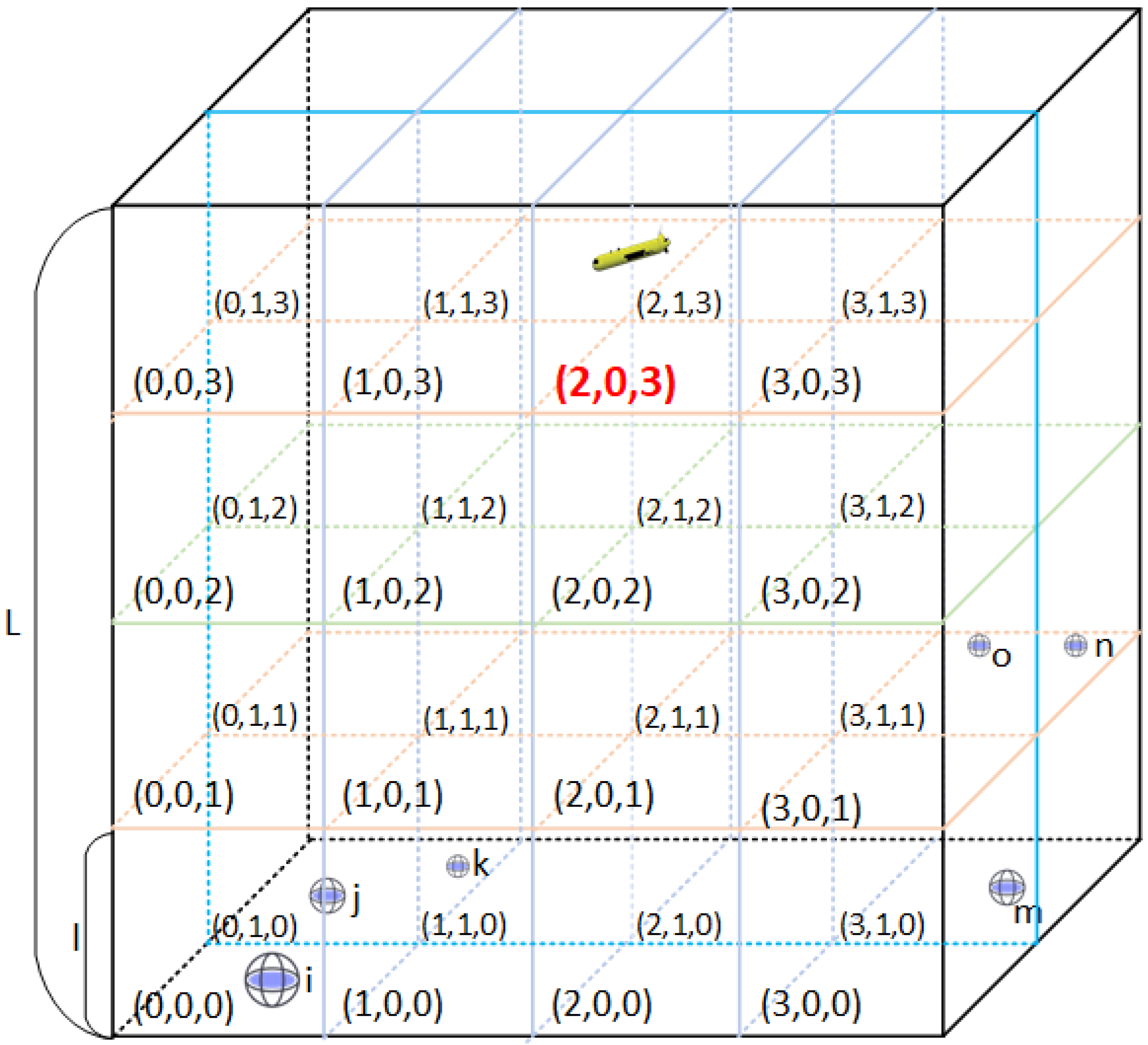
1. Sub-areas’ division

Define the edge length of cubes as L

Initialize an empty task list TsubArea to hold the sub-areas

for i in range (0,M,1):

for j in range (0,N,1):

for k in range (0,O,1):

for nodei in range (0, MAX_NODE,1):

if $T{L}_{nod{e}_i}^{subAre{a}_{ijk}}\le T{L}_{threshold}$:

Add nodei to the task list $T_{subArea}^{ijk}$

2. Sub-area Selection and the optimal order to visit nodes

While node data collection not completed:

Obtaining the optimal task through Equation (17)

Obtaining the order of traversing these nodes with the ACO algorithm.

Inform AUV of the node traversal order.

4.2. AUV-Aided Path Planning Based on Deep Reinforcement Learning

We propose an AUV-aided path planning algorithm based on DRL to guarantee high-efficiency data collection for UWSN. The AUV has its own inherited control logic that it uses to determine their trajectories for data collection. We specifically design the state, observation, action space, and reward for the AUV’s DRL model. The key advantage of DRL is its ability to learn optimal strategies in environments with severe disturbances, such as those caused by ocean currents. Unlike traditional methods [39], DRL algorithms can adapt and converge to effective strategies even in the presence of strong perturbations. This robustness is crucial for the application of AUVs.

(1) Algorithm Design: The AUV’s mission is to collect data from sensor nodes by precisely controlling its speed and heading. At each slot time t, the AUV determines its specific action $a_t$ by observing the environment $o_t$.

Observation Space: The observation capability of AUV is limited. As a result, the observation space $o_t$ of the AUV at slot time t includes the following factors: the position $\{x_t,y_t,z_t\}$ of the AUV, the velocity $\{v_t^x,v_t^y,v_t^z\}$ of the AUV, the energy consumption $e_t$ at slot time t, the residual electricity ${\epsilon }_t$, and the propagation loss $T_t^i$ of the node i. Within each time slot, the observation space of the AUV is defined as $o_t=\{x_t,y_t,z_t,v_t^x,v_t^y,v_t^z,e_t,{\epsilon }_t,T_t^i\}$. Combining these time slots, the overall observation space of the AUV is $O=\{o_1,o_2,o_3,\dots ,o_T\}$.

State Space: The data collection path planning for the AUV is a Partially Observable Markov Decision Process (POMDP) [40], where the environment is fully observable to the AUV. The state space includes all observation space $o_t$ and the data collection status $c_t$ of all sensor nodes. Combining the collection status of the nodes, the state space is defined as $S_t=\{o_t,c_t\}$.

Action Space: In the current data collection scenario, the motion of the AUV is its main activity. In the process of path planning, changes in velocity are the principal measures. Hence, the action of the AUV is $a_t=(\Delta v_t^x,\Delta v_t^y,\Delta v_t^z)$. The action space of the AUV is $A=\left\{a_t\right|t=1,2,3,\dots ,T\}$.

Reward Function: The reward function provides evaluative feedback for the AUV’s action, facilitating its decision-making improvement, which takes into account four terms: the distance between the AUV and the task center, the amount of data collected, the quality of communication between the AUV and the node, and the distance between the AUV and the boundary. The first three terms correspond to the reward functions $R_{dist}$,$R_{ic}$, and $R_{tl}$, while the fourth term corresponds to the penalty function $\zeta$.

Reward function R is calculated as follows:

$$R={\omega }_{dist}{R}_{dist}+{\omega }_{ic}{R}_{ic}-{\omega }_{tl}{R}_{tl}-{\omega }_{obs}\zeta .$$

(19)

where ${\omega }_{dist},$ ${\omega }_{ic},$ ${\omega }_{tl},$ ${\omega }_{obs}$ are weights. ${\omega }_{dist}+{\omega }_{ic}=1$, and ${\omega }_{tl}+{\omega }_{obs}=1$.

The reward $R_{dist}$ is designed to encourage the AUV to move towards the center of the sub-area and mitigate the impact of ocean currents on its position. When the AUV is further away from the center of the sub-area at time t than at time $t-1$, a penalty term will be imposed.

$$R_{dist}=-{\displaystyle \frac{{dist}_t}{{dist}_{t-1}}}.$$

(20)

where ${dist}_t$ represents the distance between the AUV and the center of the sub-area at the current time slot t; ${dist}_{t-1}$ represents the distance between the AUV and the center of the sub-area at the previous time slot $t-1$.

Incremental reward $r_{ic}$ for gathering more data. At the current time slot t, if the AUV successfully collects more data, it will be rewarded to encourage further data collection.

$$R_{ic}=\left\{\begin{array}{cc}{\delta }_{ic}\hfill & \text{if the AUV successfully collects more data,}\hfill \\ 0\hfill & \text{otherwise.}\hfill \end{array}\right.$$

(21)

where ${\delta }_{ic}$ is a fixed positive reward value for collecting more data.

The quality of the communication between the AUV and the node $r_q$. During time slot t, if the propagation loss between the AUV and the node increases, a fixed penalty will be imposed on the current action taken.

$$R_{tl}=\left\{\begin{array}{cc}{\delta }_{tl}\hfill & \text{if propagation loss increases,}\hfill \\ 0\hfill & \text{otherwise.}\hfill \end{array}\right.$$

(22)

where ${\delta }_{tl}$ is a fixed negative value representing the penalty for increased propagation loss.

If the distance between the AUV and the boundary is less than the safe distance, a fixed penalty $\zeta ={\delta }_{\zeta }$ is imposed.

(2) Training and Testing: During the training process, the AUV continuously gathers environmental information via communication and maintains communication with nodes. The training procedure for reinforcement learning is illustrated in Figure 4.

The AUV has five neural networks: Actor Network, Critic 1 Network, Critic 2 Network, Target Critic 1 Network, and Target Critic 2 Network [41]. The critic network assesses the value of the actions taken by the AUV, utilizing its current state $s_t$ and action $a_t$. Concurrently, the actor network adjusts action $a_t$ based on the value estimates provided by the critic network. The target critic network, in turn, can be updated by the critic network to forecast the subsequent state value of actions undertaken by the AUVs, given their next state $s_{t+1}$ and action $a_{t+1}$.

We first initialize two critic networks $Q_1(·),Q_2(·)$ and one actor network $\pi (·)$ with parameters ${\theta }^{Q_1},{\theta }^{Q_2}$ and ${\varphi }^{\pi }$ for the AUV. Then, two target critic networks $Q_1^{\prime }(·),Q_2^{\prime }(·)$ and target actor network $\pi {(·)}^{\prime }$ are initialized, which are the copy of their corresponding actor and critic networks with parameters.

The critic networks and the actor network are initialized with the following architecture specifications: three fully connected hidden layers with ReLU activation (256-256-1 for the critics, 256-256-3 for the actor), a Gaussian noise injection exploration strategy with $\sigma \in [e^{-20},e^2]$ for action space exploration, and soft target network updates with a Polyak averaging coefficient of $\tau =0.005$.

Next, we implement the training procedure for the AUV. At each step t, the AUV selects an action $a_t$ using the current policy $\pi (·;{\varphi }^{\pi })$, augmented with exploration noise ${ϵ}_t$. The action is executed, and the resulting state $s_{t+1}$, reward $r_t$, and done signal $d_t$ are observed and stored in a replay buffer B.

Periodically, we sample a batch of transitions $(s,a,r,s^{\prime })$ from the replay buffer B. The critic networks $Q_1(·;{\theta }^{Q_1})$ and $Q_2(·;{\theta }^{Q_2})$ are updated by minimizing the temporal difference error between their estimates and the target values computed using the target networks $Q_1^{\prime }(·;{\theta }^{Q_1^{\prime }})$ and $Q_2^{\prime }(·;{\theta }^{Q_2^{\prime }})$.

The target value is given by

$$y_t=r_t+\gamma \times \underset{i=1,2}{min}{Q}_i^{\prime }(s_{t+1},{\pi }^{\prime }(s_{t+1};{\theta }^{{\pi }^{\prime }});{\theta }_{Q^{\prime }}^{i^{\prime }}).$$

(23)

where $\gamma$ is the discount factor. The loss function for each critic network is defined as follows:

$$L_{Q_i}={\mathbb{E}}_{(s,a,r,s^{\prime })\sim B}\left[{\left(Q_i(s,a;{\theta }^{Q_i})-y_t\right)}^2\right].$$

(24)

This loss function encourages the critics to predict the target values accurately, which are based on the minimum of the two target critic networks to reduce overestimation.

The actor network is updated less frequently than the critics to maintain stability. The policy improvement step involves maximizing the expected return as estimated by one of the critic networks, typically the one with the lowest value to reduce overestimation:

$${\varphi }^{\pi }\leftarrow {\varphi }^{\pi }+\alpha {\nabla }_{{\varphi }^{\pi }}\left[Q_1(s,\pi (s;{\varphi }^{\pi });{\theta }^{Q_1})\right].$$

(25)

where $\alpha$ is the learning rate for the actor.

To stabilize learning, the target networks are updated softly by polyak averaging with the online networks:

$${\theta }^{Q_1^{\prime }}\leftarrow \tau {\theta }^{Q_1}+(1-\tau ){\theta }^{Q_1^{\prime }}.$$

(26)

$${\theta }^{Q_2^{\prime }}\leftarrow \tau {\theta }^{Q_2}+(1-\tau ){\theta }^{Q_2^{\prime }}.$$

(27)

$${\theta }^{{\pi }^{\prime }}\leftarrow \tau {\varphi }^{\pi }+(1-\tau ){\theta }^{{\pi }^{\prime }}.$$

(28)

The overall training method is shown in Algorithm 2.

Algorithm 2 Training for AUV.

Input: State $s_t$

Output: Action $a_t$

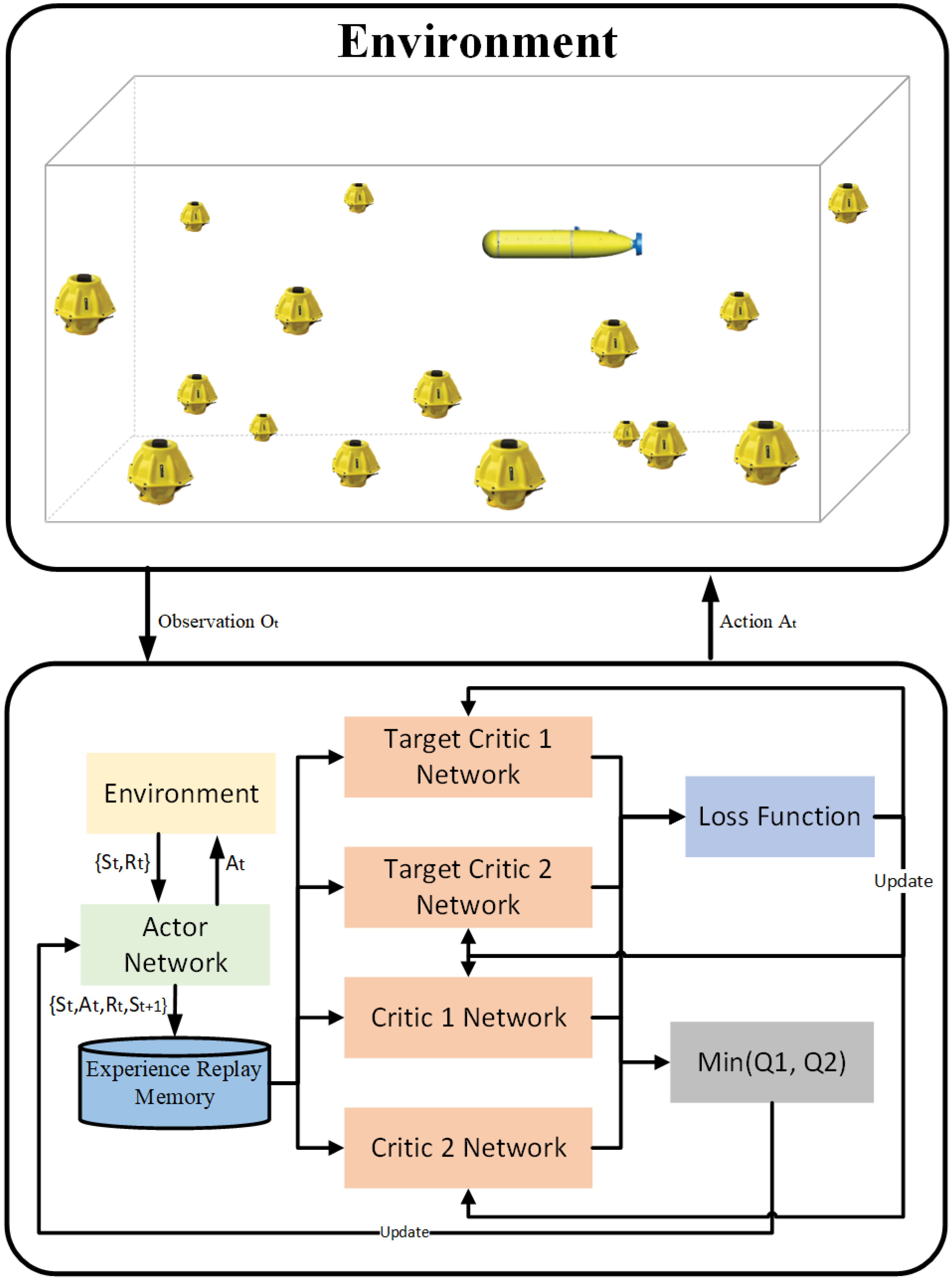
1: Initialize actor network and critic network

2: Copy target actor network and target critic network, respectively.

3: Initialize environment and receive initial observations $O_0$

4: for episode = 1, 2 …M do

5:    for $t<T$ do

6:    AUV takes action $a_t$, and gets reward $r_t$

7:    The AUV updates to a new state $s_{t+1}$

8:    Store $(s_t,a_t,r_t,s_{s+1})$ in experience replay buffer

9:    Set $s_t⟵s_{t+1}$

10:       Select N samples from experience replay buffer randomly

11:       Update critic network and actor network

12:       Update target critic network and target actor network

13:    end for

14:   end for

15: return action $a_t$

(3) Convergence and Computational Complexity Analysis: During each training iteration, CADC performs forward and backward propagation through dual critic networks and a single actor network. When considering batch size (B), total network parameters (N), and training update steps (T), the computational complexity scales linearly as follows:

$$O(B\times N\times T).$$

(29)

This complexity profile closely aligns with TD3, which similarly employs dual critics, though marginally exceeds that of DDPG due to CADC’s entropy regularization term [42]. The CADC foundation originates from the maximum entropy reinforcement learning framework, which guarantees convergence to optimal stochastic policies within the defined policy class through soft policy iteration [43].

Empirical analysis demonstrates that CADC’s entropy maximization mechanism promotes robust exploration, preventing premature convergence to suboptimal policies. Benchmark evaluations confirm that CADC consistently outperforms DDPG in both convergence speed and asymptotic performance on continuous control tasks, while frequently exceeding TD3 in policy stability and final performance metrics across underwater robotics applications [41].

5. Simulation Results

To evaluate the performance of our proposed algorithm, we performed simulations using Aqua-Sim NG [44], an open-source underwater network simulator built on NS-3 [45]. Aqua-Sim NG is a widely recognized open-source simulation tool for underwater networking, offering high-precision modeling capabilities that have been extensively validated in both academic and industrial research. We utilized ns3-gym [46], a framework that integrates the NS-3 network simulator with OpenAI Gym [47] interfaces, to implement reinforcement learning algorithms. This integration enables interactive training of DRL agents within dynamic network environments. Combined with Aqua-Sim NG’s underwater acoustic channel modeling, ns3-gym provides an efficient platform for training and validating our channel-aware path planning algorithm.

We employ a pure ALOHA [48] protocol at the MAC layer. Under this scheme, each sensor node transmits immediately whenever an MAC layer has data. If a collision occurs—retrieval is carried out after a randomly chosen backoff interval. During data collection, the AUV typically communicates point-to-point with individual node, making the “transmit-on-arrival” nature of ALOHA especially well suited to our network scenario.

In this section, we first introduce the setting of the simulation experiment in detail, including the environment and algorithm parameters. Second, we conduct a large number of experimental results to demonstrate the process of AUV data collection tasks and verify the feasibility of proposed CADC algorithm. Finally, we compare CADC with the baseline algorithm in different task environments.

5.1. Experiment Settings

Environment Parameters

We initially deploy 200 sensor nodes in a 5 km × 5 km × 1 km area at random (assuming sensor nodes on the seabed) and assume an AUV in this area. The velocity $\widehat{v}$ of the AUV relative to the Earth’s coordinate system is the vector sum of its navigation velocity $v^n=\{v_x^n,v_y^n,v_z^n\}$ and the ocean current speed $v^c=\{v_x^c,v_y^c,v_z^c\}$, i.e., $\widehat{v}=v^n+v^c$.

5.2. Algorithm Parameters

In terms of path planning, we conducted a multitude of experimental simulations to identify the optimal parameters for CADC. In the training stage, the step T = 0.1 s [46]. The learning rates for the actor network and critic network are set to $3\times {10}^{-4}$ and $3\times {10}^{-4}$, respectively. The discount factor $\gamma$ was assigned a value of $0.99$ to balance the weight between immediate rewards and future rewards. To facilitate network updates, the soft update coefficient $\tau$ is set to $0.005$ [49].

5.3. Simulation Results and Analysis

Based on reinforcement learning framework, the AUV is trained with the CADC algorithm to optimize policy. At the beginning of each epoch, the position of the AUV and the status of nodes will be reset. The AUV selects a target sub-area and target node [38]. The AUV then navigates to the target sub-area for data collection. Once the data of the node is collected, the AUV will reselect the next node and repeat the above process until the task is completed.

5.3.1. Comparison of Energy-Saving Performance

To comprehensively validate the energy-saving performance of CADC in practical underwater scenarios, we first evaluate its energy efficiency (defined in Equation (10)) under ocean currents.

We compare CADC with DDPG [50], TD3 [42], cluster-based path planning [14], and pre-designated path planning [4]. DDPG is an advanced algorithm that combines deep learning and reinforcement learning. By leveraging deep neural networks to approximate policy functions and value functions, DDPG can effectively learn optimal policies in continuous action spaces, thereby achieving efficient decision making and control in complex environments. TD3 addresses the overestimation issue of action Q-values by the critic in DDPG through the introduction of a dual critic network. Furthermore, TD3 employs a method of delayed policy network updates to reduce the value estimation variance caused by accumulated TD errors. Lastly, TD3 introduces Gaussian noise into the target policy to achieve target policy smoothing, thereby enhancing the stability of the algorithm. The cluster-based method utilizes the k-means clustering algorithm to partition the nodes into several clusters and select the cluster heads. The AUV traverses these cluster heads along a planned route, collects the data, and uploads it to the surface base station. The pre-designated method divides the entire task area into several sub-areas. The AUV follows a predetermined fixed route, successively arriving at each sub-area, and collects data from all nodes within that sub-area.

Experimental results demonstrate that CADC exhibits a higher energy efficiency than DDPG and TD3, validating its advantage in energy conservation. As shown in Figure 5, CADC achieves peak energy efficiency after 81,179 training steps, reducing convergence time by 18.5% and 2.3% compared to DDPG (99,737 steps) and TD3 (83,092 steps), respectively. In the initial phase, exploration strategies lead to a general decline in energy efficiency. During the intermediate phase, path optimization capability determines the convergence rate, while in the later phase, the sparse distribution of nodes constrains the upper bound of efficiency improvement. CADC maintains overall superior energy efficiency after training completion.

As shown in

Table 1. Comparisons of energy efficiency among baseline methods and CADC.

	Execution Steps	Energy Efficiency (J/byte)
DDPG	99,737	0.03528
TD3	83,092	0.035254
CADC	81,179	0.035254
pre-specified	555,620	0.05146
clustering-based	95,018	0.12210

, CADC significantly outperforms traditional data collection methods (pre-specified paths, clustering-based schemes) and mainstream reinforcement learning algorithms (DDPG, TD3) in both energy efficiency and execution efficiency. The pre-specified path planning method uses a fixed trajectory, ignoring the dynamic distribution of underwater nodes and the time-varying nature of the acoustic channel. This leads to redundant path traversal and reveals the environmental adaptation limitations of rigid strategies. Clustering-based methods rely on high-power cluster head nodes for data relaying. The extra communication energy consumption lowers their energy efficiency. CADC has a maximum energy efficiency of 0.035254 J/byte and can finish data collection in 81,179 steps. In comparison, the preset path method has an energy efficiency of 0.05146 J/Byte, roughly 1.5 times that of CADC. Moreover, the energy consumption of the cluster-based method is 3.46 times that of CADC.

In underwater sensor networks of various scales (50–200 nodes), the CADC algorithm shows remarkable energy-saving features, with its energy efficiency improving regularly as the network scale expands. As indicated in

Table 2. Energy efficiency (J/byte) under different nodes.

Number of Nodes	Execution Steps	Energy Efficiency
50	58,577	0.0751
100	88,636	0.0589
150	94,026	0.046
200	81,179	0.0352

, when the node count increases from 50 to 200, energy efficiency decreases steadily from 0.0751 J/byte to 0.0352 J/byte, highlighting the algorithm’s strong scalability in large-scale situations.

5.3.2. Comparison with Proximity-Based TSP Data Collection Methods

In many AUV-assisted data collection studies, the AUV must first position itself within a predefined effective range of each sensor node to initiate data transfer. Such approaches typically solve a Traveling Salesman Problem (TSP) over all nodes, visiting them in an optimal sequence while ensuring the AUV enters the communication zone of each target node before collection. We implemented this classic TSP scheme as a baseline: after computing the optimal tour, the AUV navigates to sequential nodes and commences data collection.

Figure 6 compares the energy cost of CADC against a TSP-based method, clearly showing that CADC requires only 77.8% of the energy cost of the TSP approaches, thereby underscoring the importance of channel awareness in data collection.

5.3.3. Accumulated Reward and Algorithm Stability

Figure 7 shows that the CADC algorithm shows the best accumulated reward performance in AUV underwater data collection tasks. During the initial training phase, the cumulative reward increases rapidly and then stabilizes, indicating that the AUV quickly finds effective strategies during the learning process and achieves near-optimal performance after a period. The two brief drops in reward for TD3 may be due to delayed updates in its critic network, resulting in insufficient adaptability to ocean current disturbances. DDPG, due to Q-value overestimation by its single critic network, causes the AUV to take excessive risks in scenarios with fewer nodes, leading to energy waste and requiring additional training. In conclusion, the experimental results demonstrate that CADC effectively achieves high cumulative rewards while maintaining stability. This makes CADC particularly suitable for tasks that require long-term planning and dynamic adaptation.

Table 1 and

Table 3. Comparisons of PDR.

	DDPG	TD3	CADC	Pre-Specified	Clustering-Based
execution steps	99,737	83,092	81,179	555,620	95,018
PDR	0.96538	0.96706	0.95288	1.0	0.94206

together illustrate that different data collection algorithms present a significant trade-off between the packet delivery rate (PDR) and energy efficiency. Although the pre-specified approach has perfect PDR data, its rigid path planning leads to a high number of execution steps (555,620) and a severe reduction in energy efficiency. The clustering-based approach, which relies on cluster-head nodes for data relaying, also reduces its PDR to 0.94206. CADC achieves full data collection with minimum energy consumption by combining dynamic channel sensing with reinforcement learning path planning while maintaining a high PDR (0.95288), which validates its comprehensive performance advantages in complex underwater environments. Reinforcement learning-based algorithms, including CADC, achieve an optimal balance between PDR and energy efficiency. This balance is particularly suitable for underwater long-term monitoring scenarios (e.g., deep-sea mining environment monitoring) with battery constraints and high channel dynamics.

CADC has the best collection rate, followed by TD3 and DDPG. CADC has fast convergence and high training stability. As shown in Figure 8, the collection rate curve of CADC rises rapidly in the early stage, indicating its ability to quickly adapt to the environment and find effective data collection strategies. After reaching a high collection rate, the curve stabilizes, showing stable performance during training and continuous effective data collection. In contrast, the TD3 algorithm’s curve also rises but with larger fluctuations, indicating weaker adaptability during training. It stabilizes later but at a slightly lower collection rate than CADC. The DDPG algorithm’s curve rises but remains below CADC and TD3, with larger fluctuations, indicating poorer adaptability in complex environments. Experimental results show that CADC achieves a high collection rate while maintaining stability, making it ideal for tasks requiring long-term planning and dynamic adaptation, such as AUV underwater data collection. Although TD3 and DDPG can also complete tasks, they perform worse than CADC in terms of the collection rate and stability.

6. Conclusions

In this paper, we have introduced the CADC algorithm, an innovative data collection scheme for AUVs operating within underwater sensor networks. This algorithm leverages DRL to enhance both data collection efficiency and reduce energy consumption. We designed an effective underwater node traversal algorithm that takes into account the unique propagation characteristics of underwater channels, thereby improving data collection efficiency. Additionally, we proposed a DRL-based path planning algorithm that addresses underwater propagation losses, allowing AUVs to adapt to dynamic underwater environments while minimizing network energy consumption. Our study presents a new solution for optimizing data collection in underwater settings, a critical aspect for advancing marine exploration and monitoring technologies. Extensive simulation experiments have shown that CADC outperforms existing state-of-the-art methods, including DDPG, TD3, clustering-based approaches, and pre-specified path planning strategies, across metrics such as energy efficiency, accumulated rewards, and data collection rates. Future research could aim to further enhance the algorithm’s adaptability to more complex underwater environments and explore its application in multi-AUV collaborative scenarios.

References

1. Martin, C.; Weilgart, L.; Amon, D.; Müller, J. Deep-Sea Mining: A Noisy Affair—Overview and Recommendations. 2021. Available online: https://www.oceancare.org/wp-content/uploads/2021/12/Deep-Sea-Mining_A-noisy-affair_Report-OceanCare_2021.pdf (accessed on 19 March 2025).
2. Cheng, M.; Guan, Q.; Ji, F.; Cheng, J.; Chen, Y. Dynamic-detection-based trajectory planning for autonomous underwater vehicle to collect data from underwater sensors. IEEE Internet Things J. 2022, 9, 13168–13178. [Google Scholar] [CrossRef]
3. Koschinsky, A.; Heinrich, L.; Boehnke, K.; Cohrs, J.C.; Markus, T.; Shani, M.; Singh, P.; Smith Stegen, K.; Werner, W. Deep-sea mining: Interdisciplinary research on potential environmental, legal, economic, and societal implications. Integr. Environ. Assess. Manag. 2018, 14, 672–691. [Google Scholar] [CrossRef] [PubMed]
4. Jiang, J.; Tian, W.; Han, G.; Zhang, F. A Medium Access Control Protocol Based on Parity Group-Graph Coloring for Underwater AUV-Aided Data Collection. IEEE Internet Things J. 2024, 11, 5967–5979. [Google Scholar] [CrossRef]
5. Porter, M.B. The Bellhop Manual and User’s Guide: Preliminary Draft; Tech. Rep. Heat, Light, and Sound Research, Inc.: La Jolla, CA, USA, 2011; Volume 260. [Google Scholar]
6. Chen, M.; Zhu, D. Data collection from underwater acoustic sensor networks based on optimization algorithms. Computing 2020, 102, 83–104. [Google Scholar] [CrossRef]
7. Che, S.; Song, S.; Xu, C.; Liu, J.; Cui, J.H. ACARP: An Adaptive Channel-Aware Routing Protocol for Underwater Wireless Sensor Networks. In Proceedings of the 2023 IEEE/CIC International Conference on Communications in China (ICCC), Dalian, China, 10–12 August 2023; pp. 1–6. [Google Scholar] [CrossRef]
8. Jiang, Q.; Zhu, R.; Boukerche, A.; Yang, Q. An AUV-Assisted Data Collection Approach for UASNs Based on Hybrid Clustering and Matrix Completion. In Proceedings of the 2024 IEEE Wireless Communications and Networking Conference (WCNC), Dubai, United Arab Emirates, 21–24 April 2024; pp. 1–6. [Google Scholar] [CrossRef]
9. Guo, Z.; Colombi, G.; Wang, B.; Cui, J.H.; Maggiorini, D.; Rossi, G.P. Adaptive Routing in Underwater Delay/Disruption Tolerant Sensor Networks. In Proceedings of the 2008 Fifth Annual Conference on Wireless on Demand Network Systems and Services, Garmisch-Partenkirchen, Germany, 23–25 January 2008; pp. 31–39. [Google Scholar] [CrossRef]
10. Di Valerio, V.; Lo Presti, F.; Petrioli, C.; Picari, L.; Spaccini, D.; Basagni, S. CARMA: Channel-Aware Reinforcement Learning-Based Multi-Path Adaptive Routing for Underwater Wireless Sensor Networks. IEEE J. Sel. Areas Commun. 2019, 37, 2634–2647. [Google Scholar] [CrossRef]
11. Wang, J.; Liu, S.; Shi, W.; Han, G.; Yan, S. A Multi-AUV Collaborative Ocean Data Collection Method Based on LG-DQN and Data Value. IEEE Internet Things J. 2024, 11, 9086–9106. [Google Scholar] [CrossRef]
12. Hao, Z.; Li, W.; Zhang, Q. Efficient Clustering Data Collection in AUV-Aided Underwater Sensor Network. In Proceedings of the OCEANS 2023—MTS/IEEE U.S. Gulf Coast, Biloxi, MS, USA, 25–28 September 2023; pp. 1–6. [Google Scholar] [CrossRef]
13. Li, Y.; Huang, H.; Zhuang, Y.; Chen, Z.; Wang, X.; Xu, X. Multi-AUV Collaborative Data Collection Scheme to Clustering and Routing for Heterogeneous UWSNs. IEEE Sens. J. 2024, 24, 42289–42301. [Google Scholar] [CrossRef]
14. Liu, Z.; Liang, Z.; Yuan, Y.; Chan, K.Y.; Guan, X. Energy-Efficient Data Collection Scheme Based on Value of Information in Underwater Acoustic Sensor Networks. IEEE Internet Things J. 2024, 11, 18255–18265. [Google Scholar] [CrossRef]
15. Liu, Z.; Meng, X.; Liu, Y.; Yang, Y.; Wang, Y. AUV-Aided Hybrid Data Collection Scheme Based on Value of Information for Internet of Underwater Things. IEEE Internet Things J. 2022, 9, 6944–6955. [Google Scholar] [CrossRef]
16. Yan, J.; Yang, X.; Luo, X.; Chen, C. Energy-Efficient Data Collection Over AUV-Assisted Underwater Acoustic Sensor Network. IEEE Syst. J. 2018, 12, 3519–3530. [Google Scholar] [CrossRef]
17. Ding, Y.; Wang, X.; Xu, J.; Xie, G.; Liu, W.; Li, Y. Multi-Objective-Optimization Multi-AUV Assisted Data Collection Framework for IoUT Based on Offline Reinforcement Learning. arXiv 2024. [Google Scholar] [CrossRef]
18. Jiang, B.; Du, J.; Ren, K.; Jiang, C.; Han, Z. Multi-Agent Reinforcement Learning based Secure Searching and Data Collection in AUV Swarms. In Proceedings of the ICC 2023—IEEE International Conference on Communications, Rome, Italy, 28 May–1 June 2023; pp. 5085–5090. [Google Scholar] [CrossRef]
19. Bu, F.; Luo, H.; Ma, S.; Li, X.; Ruby, R.; Han, G. AUV-Aided Optica-Acoustic Hybrid Data Collection Based on Deep Reinforcement Learning. Sensors 2023, 23, 578. [Google Scholar] [CrossRef] [PubMed]
20. Busacca, F.; Galluccio, L.; Palazzo, S.; Panebianco, A.; Raftopoulos, R. AMUSE: A Multi-Armed Bandit Framework for Energy-Efficient Modulation Adaptation in Underwater Acoustic Networks. IEEE Open J. Commun. Soc. 2025, 6, 2766–2779. [Google Scholar] [CrossRef]
21. Zhang, Y.; Zhu, J.; Liu, Y.; Wang, B. Underwater Acoustic Adaptive Modulation with Reinforcement Learning and Channel Prediction. In Proceedings of the 15th International Conference on Underwater Networks & Systems, WUWNet ’21, Shenzhen, China, 22–24 November 2021; Association for Computing Machinery: New York, NY, USA, 2022. [Google Scholar] [CrossRef]
22. Su, W.; Lin, J.; Chen, K.; Xiao, L.; En, C. Reinforcement Learning-Based Adaptive Modulation and Coding for Efficient Underwater Communications. IEEE Access 2019, 7, 67539–67550. [Google Scholar] [CrossRef]
23. Cheng, C.F.; Li, L.H. Data gathering problem with the data importance consideration in Underwater Wireless Sensor Networks. J. Netw. Comput. Appl. 2017, 78, 300–312. [Google Scholar] [CrossRef]
24. Shahapur, S.S.; Khanai, R. Localization, routing and its security in UWSN—A survey. In Proceedings of the 2016 International Conference on Electrical, Electronics, and Optimization Techniques (ICEEOT), Chennai, India, 3–5 March 2016; pp. 1001–1006. [Google Scholar] [CrossRef]
25. Song, S.; Liu, J.; Guo, J.; Lin, B.; Ye, Q.; Cui, J. Efficient Data Collection Scheme for Multi-Modal Underwater Sensor Networks Based on Deep Reinforcement Learning. IEEE Trans. Veh. Technol. 2023, 72, 6558–6570. [Google Scholar] [CrossRef]
26. Gul, S.; Zaidi, S.S.H.; Khan, R.; Wala, A.B. Underwater acoustic channel modeling using BELLHOP ray tracing method. In Proceedings of the 2017 14th International Bhurban Conference on Applied Sciences and Technology (IBCAST), Islamabad, Pakistan, 10–14 January 2017; pp. 665–670. [Google Scholar] [CrossRef]
27. Cheng, M.; Guan, Q.; Wang, Q.; Ji, F.; Quek, T.Q.S. FER-Restricted AUV-Relaying Data Collection in Underwater Acoustic Sensor Networks. IEEE Trans. Wirel. Commun. 2023, 22, 9131–9142. [Google Scholar] [CrossRef]
28. Shehwar, D.E.; Gul, S.; Zafar, M.U.; Shaukat, U.; Syed, A.H.; Zaidi, S.S.H. Acoustic Wave Analysis In Deep Sea And Shallow Water Using Bellhop Tool. In Proceedings of the 2021 OES China Ocean Acoustics (COA), Harbin, China, 14–17 July 2021; pp. 331–334. [Google Scholar] [CrossRef]
29. Awan, K.M.; Shah, P.A.; Iqbal, K.; Gillani, S.; Ahmad, W.; Nam, Y. Underwater Wireless Sensor Networks: A Review of Recent Issues and Challenges. Wirel. Commun. Mob. Comput. 2019, 2019, 6470359. [Google Scholar] [CrossRef]
30. Felemban, E.; Shaikh, F.K.; Qureshi, U.M.; Sheikh, A.A.; Qaisar, S.B. Underwater Sensor Network Applications: A Comprehensive Survey. Int. J. Distrib. Sens. Netw. 2015, 11, 896832. [Google Scholar] [CrossRef]
31. Urick, R.J. Principles of Underwater Sound, 3rd ed.; McGraw-Hill: New York, NY, USA, 1983. [Google Scholar]
32. Wang, Y.; Liu, K.; Geng, L.; Zhang, S. Knowledge hierarchy-based dynamic multi-objective optimization method for AUV path planning in cooperative search missions. Ocean. Eng. 2024, 312, 119267. [Google Scholar] [CrossRef]
33. Han, G.; Jiang, J.; Shu, L.; Guizani, M. An Attack-Resistant Trust Model Based on Multidimensional Trust Metrics in Underwater Acoustic Sensor Network. IEEE Trans. Mob. Comput. 2015, 14, 2447–2459. [Google Scholar] [CrossRef]
34. Zhou, S.; Wang, Z. OFDM for Underwater Acoustic Communications, 1st ed.; John Wiley & Sons: Hoboken, NJ, USA, 2014. [Google Scholar]
35. Garau, B.; Alvarez, A.; Oliver, G. AUV navigation through turbulent ocean environments supported by onboard H-ADCP. In Proceedings of the 2006 IEEE International Conference on Robotics and Automation, ICRA 2006, Orlando, FL, USA, 15–19 May 2006; pp. 3556–3561. [Google Scholar] [CrossRef]
36. Zhang, T.; Gou, Y.; Liu, J.; Yang, T.; Cui, J.H. UDARMF: An Underwater Distributed and Adaptive Resource Management Framework. IEEE Internet Things J. 2022, 9, 7196–7210. [Google Scholar] [CrossRef]
37. Han, G.; Li, S.; Zhu, C.; Jiang, J.; Zhang, W. Probabilistic Neighborhood-Based Data Collection Algorithms for 3D Underwater Acoustic Sensor Networks. Sensors 2017, 17, 316. [Google Scholar] [CrossRef]
38. Dorigo, M.; Birattari, M.; Stutzle, T. Ant colony optimization. IEEE Comput. Intell. Mag. 2006, 1, 28–39. [Google Scholar] [CrossRef]
39. Cheng, C.; Sha, Q.; He, B.; Li, G. Path planning and obstacle avoidance for AUV: A review. Ocean. Eng. 2021, 235, 109355. [Google Scholar] [CrossRef]
40. Lauri, M.; Hsu, D.; Pajarinen, J. Partially Observable Markov Decision Processes in Robotics: A Survey. IEEE Trans. Robot. 2023, 39, 21–40. [Google Scholar] [CrossRef]
41. Haarnoja, T.; Zhou, A.; Abbeel, P.; Levine, S. Soft Actor-Critic: Off-Policy Maximum Entropy Deep Reinforcement Learning with a Stochastic Actor. In Proceedings of the 35th International Conference on Machine Learning, Stockholm, Sweden, 10–15 July 2018; Dy, J., Krause, A., Eds.; Proceedings of Machine Learning Research (PMLR). Volume 80, pp. 1861–1870. [Google Scholar]
42. Fujimoto, S.; van Hoof, H.; Meger, D. Addressing Function Approximation Error in Actor-Critic Methods. arXiv 2018. [Google Scholar] [CrossRef]
43. Matheron, G.; Perrin, N.; Sigaud, O. The problem with DDPG: Understanding failures in deterministic environments with sparse rewards. arXiv 2019. [Google Scholar] [CrossRef]
44. Martin, R.; Rajasekaran, S.; Peng, Z. Aqua-Sim Next Generation: An NS-3 Based Underwater Sensor Network Simulator. In Proceedings of the 12th International Conference on Underwater Networks & Systems, WUWNet ’17, Halifax, NS, Canada, 6–8 November 2017. [Google Scholar] [CrossRef]
45. Riley, G.F.; Henderson, T.R. The ns-3 Network Simulator. In Modeling and Tools for Network Simulation; Wehrle, K., Güneş, M., Gross, J., Eds.; Springer: Berlin/Heidelberg, Germany, 2010; pp. 15–34. [Google Scholar] [CrossRef]
46. Gawlowicz, P.; Zubow, A. ns3-gym: Extending OpenAI Gym for Networking Research. arXiv 2018. [Google Scholar] [CrossRef]
47. Brockman, G.; Cheung, V.; Pettersson, L.; Schneider, J.; Schulman, J.; Tang, J.; Zaremba, W. OpenAI Gym. arXiv 2016. [Google Scholar] [CrossRef]
48. Chirdchoo, N.; Soh, W.S.; Chua, K.C. Aloha-Based MAC Protocols with Collision Avoidance for Underwater Acoustic Networks. In Proceedings of the IEEE INFOCOM 2007—26th IEEE International Conference on Computer Communications, Anchorage, AK, USA, 6–12 May 2007; pp. 2271–2275. [Google Scholar] [CrossRef]
49. Padhye, V.; Lakshmanan, K. A deep actor critic reinforcement learning framework for learning to rank. Neurocomputing 2023, 547, 126314. [Google Scholar] [CrossRef]
50. Lillicrap, T.P.; Hunt, J.J.; Pritzel, A.; Heess, N.; Erez, T.; Tassa, Y.; Silver, D.; Wierstra, D. Continuous control with deep reinforcement learning. arXiv 2019. [Google Scholar] [CrossRef] [PubMed]
Figure 1. The scenario of data collection by a single AUV.
Jmse 13 01460 g001
Figure 3. Network partition based on 3D spatial gridding for channel-aware data collection.
Jmse 13 01460 g003
Figure 4. Architecture for AUV data collection.
Jmse 13 01460 g004
Figure 5. Evolution of global energy cost (EC) during training.
Jmse 13 01460 g005
Figure 6. Comparison of energy cost between CADC and TSP-based algorithm.
Jmse 13 01460 g006
Figure 7. Accumulated reward during training.
Jmse 13 01460 g007
Figure 8. Collection rate during training.
Jmse 13 01460 g008