Efficient Modeling of Underwater Target Radiation and Propagation Sound Field in Ocean Acoustic Environments Based on Modal Equivalent Sources

Abstract

The equivalent source method (ESM) is a core algorithm in integrated radiation-propagation acoustic field modeling. However, in challenging marine environments, including deep-sea and polar regions, where sound speed profiles exhibit strong vertical gradients, the ESM must increase waveguide stratification to maintain accuracy. This causes computational costs to scale exponentially with the number of layers, compromising efficiency and limiting applicability. To address this, this paper proposes a modal equivalent source (MES) model employing normal modes as basis functions instead of free-field Green’s functions. This model constructs a set of normal mode bases using full-depth hydroacoustic parameters, incorporating water column characteristics into the basis functions to eliminate waveguide stratification. This significantly reduces the computational matrix size of the ESM and computes acoustic fields in range-dependent waveguides using a single set of normal modes, resolving the dual limitations of inadequate precision and low efficiency in such environments. Concurrently, for the construction of basis functions, this paper also proposes a fast computation method for eigenvalues and eigenmodes in waveguide contexts based on phase functions and difference equations. Furthermore, coupling the MES method with the Finite Element Method (FEM) enables integrated computation of underwater target radiation and propagation fields. Multiple simulations demonstrate close agreement between the proposed model and reference results (errors < 4 dB). Under equivalent accuracy requirements, the proposed model reduces computation time to less than 1/25 of traditional ESM, achieving significant efficiency gains. Additionally, sea trial verification confirms model effectiveness, with mean correlation coefficients exceeding 0.9 and mean errors below 5 dB against experimental data.

1. Introduction

Efficient computational methods for vibroacoustic coupling, acoustic radiation, and sound propagation of elastic structural targets, such as surface ships and underwater vehicles, constitute a critical area in applying underwater acoustic technologies to marine engineering. Accurate prediction of radiation and propagation acoustic fields from these structural sources is essential to reveal their propagation characteristics in underwater environments, thereby providing scientific foundations for target noise level assessment, rapid identification, and other related engineering applications ([1,2]). The acoustic field of a target in the marine environment is inherently a coupled radiation and propagation process (Chen et al. [3], Jiang et al. [4], Huang et al. [5], Zhang et al. [6]). However, early studies on acoustic field modeling primarily focused on two separate aspects: vibroacoustic radiation computation from vibrating structures (Zhou and Joseph [7], Frendi et al. [8], Duan et al. [9]), and sound propagation modeling in oceanic waveguides (Pekeris [10], Jensen et al. [11]). The former emphasizes the radiation characteristics of targets and their influencing factors, while the latter focuses on acoustic field modeling in diverse marine waveguides and the impact of underwater environments on propagation properties. Additionally, constrained by computational capabilities, early coupled models were typically limited to simple waveguide environments. With growing application demands, an increasing number of studies now explore integrated acoustic field computation in range dependent underwater acoustic environments (Lim and Ozard [12], Oba [13], Holland [14], He et al. [15]).

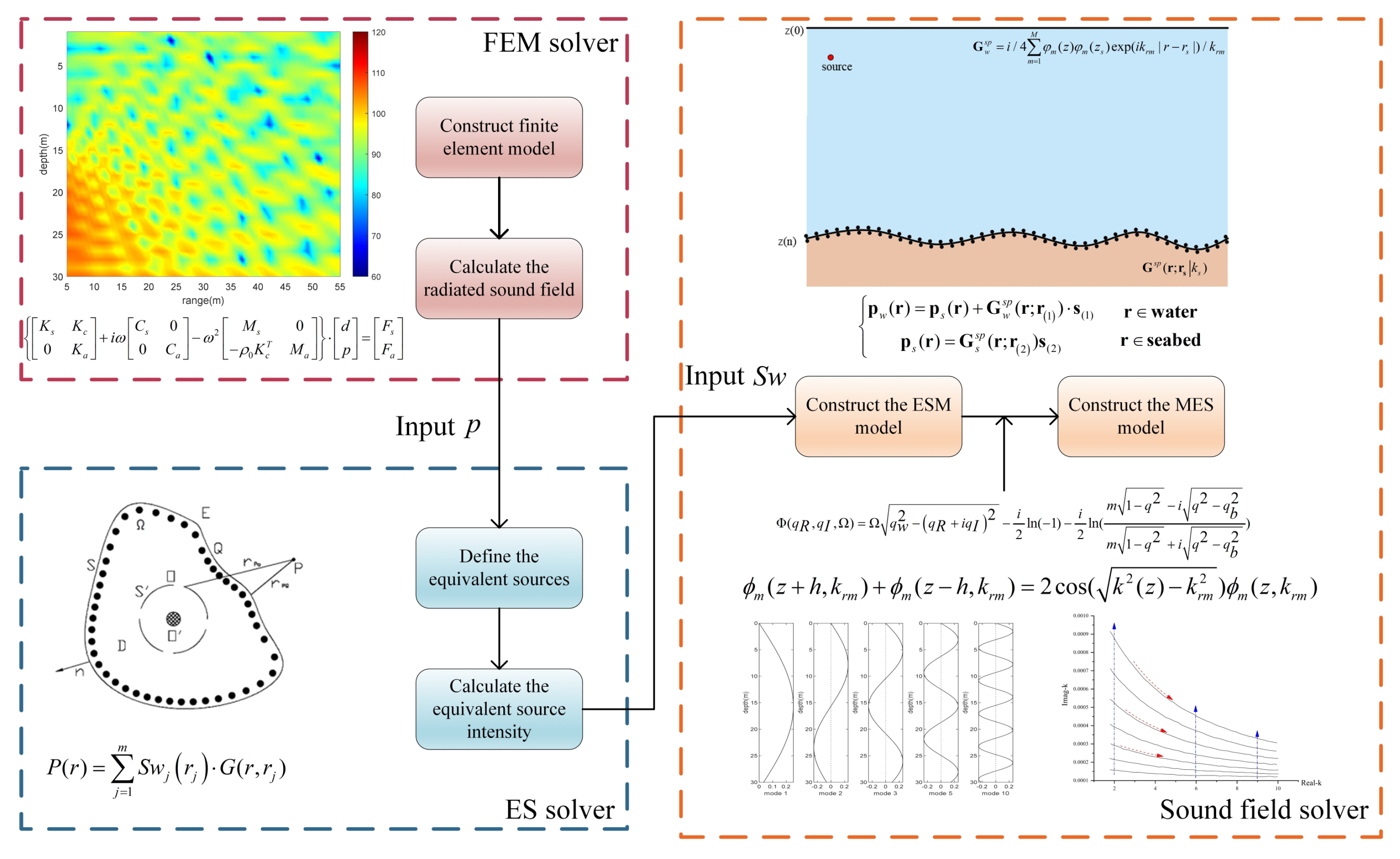
The core of coupled radiation and propagation computation for target acoustic fields lies in integrating the vibrational response of the target structure with radiation source based propagation models. Structural responses are typically resolved through analytical or numerical methods, whereas propagation fields require solving the Helmholtz equation. The widely used Finite Element Method/Boundary Element Method (FEM/BEM) framework employs FEM for target vibroacoustic radiation analysis and BEM for propagation field modeling. Leveraging FEM’s numerical precision, FEM/BEM has proven effective in applications like surface ship noise prediction and underwater structural target acoustic field calculations (Zheng et al. [16], Peters et al. [17], Li et al. [18], Chen et al. [19]). However, FEM/BEM faces limitations, particularly in BEM’s restricted capability to model propagation fields in non free field environments. Previous studies (Jiang et al. [4], Zhang et al. [6], Zou et al. [20]) addressed this limitation by modifying boundary integral equation Green’s functions to analyze ideal waveguide propagation. However, these methods depend on Green’s functions formulated for shallow water environments with parallel boundaries, rendering them impractical for range dependent waveguides. To overcome this limitation, researchers (Huang et al. [5], He et al. [15], Zou et al. [21]) introduced methods to extract equivalent radiation source terms from target vibrational responses or radiated fields, enabling propagation modeling in range dependent environments. Following this paradigm, this work reconstructs target radiated fields as superpositions of equivalent source fields. The equivalent source strengths are extracted from the radiated fields computed via FEM and subsequently fed into propagation models for propagation acoustic field computation.

To achieve efficient sound propagation computation in range dependent waveguides, it is essential to effectively couple appropriate propagation models with radiation models. Classical propagation models include normal mode, parabolic equation, ray theory, and virtual source models. Among these, virtual source models are widely used in simple waveguides with parallel boundaries (e.g., ideal or Pekeris waveguides (Jiang et al. [4], Huang et al. [5], Zhang et al. [6])) due to their low complexity and high computational speed. However, their reliance on plane wave reflection approximations restricts applicability (Gao et al. [22]). Ray theory, as high frequency approximations of the Helmholtz equation, originated from geometric acoustics and can explain sound propagation in certain real world environments (Gul et al. [23], Porter [24]). Yet, it face challenges in handling complex structural sources and environments: calculating eigenrays becomes computationally intensive, while caustic regions, bottom slope discontinuities, and boundary reflection coefficient uncertainties degrade prediction accuracy (Porter [24]). Parabolic equations improve computational efficiency via paraxial approximations of the Helmholtz equation, neglecting backward scattering, and have been successfully applied to range dependent environments (Jensen and Kuperman [25], Lin [26], Sturm [27]). Despite their flexibility in source type handling, the choice of operator expansion order and reference wavenumber significantly affects near field aperture angles and far field phase errors (Jensen et al. [11]). Additionally, abrupt environmental variations may compromise their accuracy. Normal mode represents exact solutions to wave equations under specific boundary conditions. Although inherently limited to range independent problems, coupled normal mode methods decompose range dependent waveguides into range independent segments. By enforcing boundary conditions at each segment interface, a global coupling matrix is constructed to solve the acoustic field (Preisig and Duda [28], Athanassoulis et al. [29], Tu et al. [30]). Despite high accuracy, this approach suffers from inefficiency due to repeated eigenvalue and eigenfunction computations across segments.

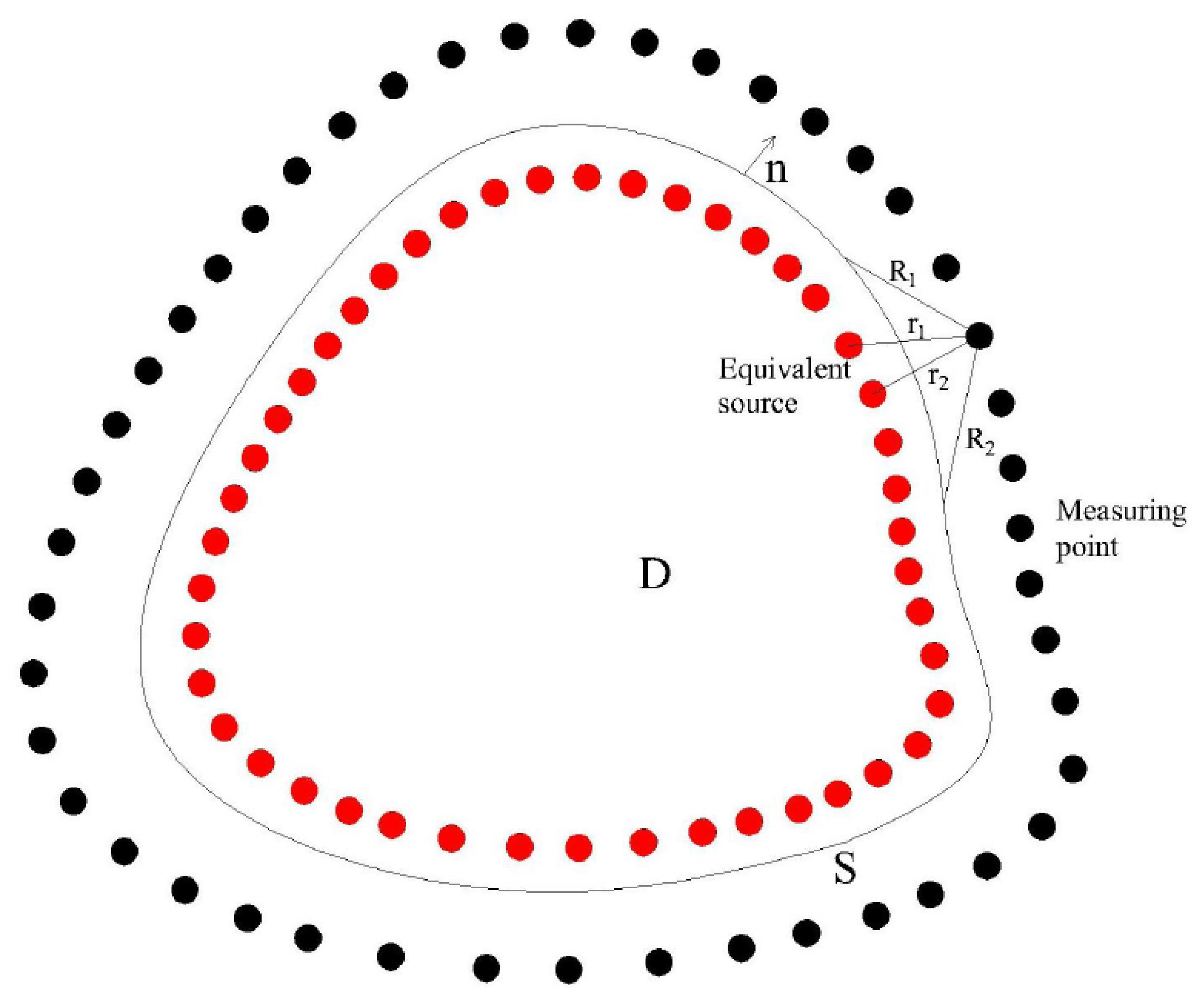
Beyond the aforementioned methods, the ESM have been extensively verified and applied to acoustic field calculations in range dependent waveguides (Abawi and Porter [31], He et al. [32]). The ESM replaces boundary reflected and transmitted sound fields by superimposing basis functions (Green’s functions) generated from equivalent sources to solve the Helmholtz equation rigorously. This method characterizes acoustic reflection and transmission at media interfaces through continuity conditions, avoiding errors and angular dependencies inherent in equivalent reflection coefficients, thereby achieving high computational accuracy. By vertical stratifying waveguides based on water column parameters, ESM simplifies modeling of complex underwater acoustic environments. However, for depth-dependent hydrological parameters, its accuracy and efficiency are highly sensitive to the number and spatial distribution of equivalent sources. Insufficient vertical stratification layers degrade accuracy if mismatched with the water column’s vertical discretization requirements. As the number of layers increases, the computational matrix size of equivalent sources grows as ${(1+2N_w·N_s)}^2$ ($N_w$ is number of water layers, $N_s$ is equivalent sources per layer). To mitigate these issues, recent studies proposed replacing free field Green’s functions with Helmholtz compliant basis functions (He et al. 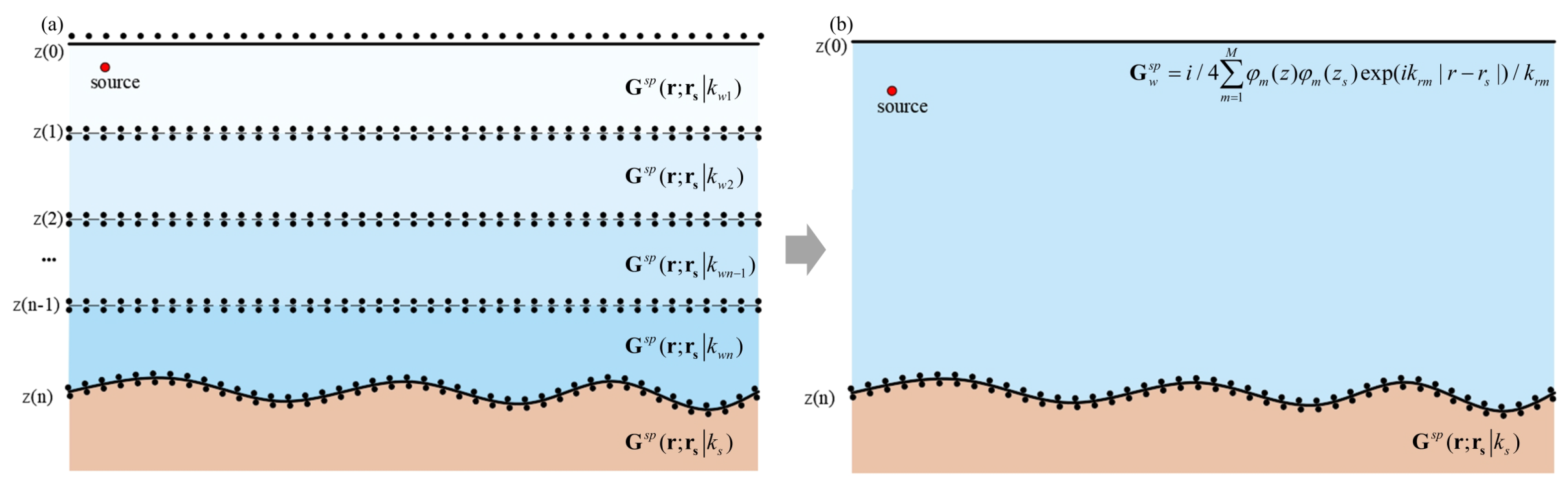[33]). Building on this, our work introduces normal mode based basis functions to replace conventional free field Green’s functions in ESM. By embedding water column parameters into basis functions, the equivalent source matrix size remains fixed at ${\left(2N_s\right)}^2$, eliminating computational inefficiencies caused by vertical layering. Additionally, an equivalent waveguide is employed to solve for the eigenvalues and eigenmodes corresponding to the actual waveguide, while introducing a computationally efficient solution method for these eigenproblems.

To address limitations of traditional ESM in range-dependent waveguides with depth-dependent hydroacoustic parameters, such as deep-sea and polar regions, this study proposes a MES model and develops an integrated radiation-propagation computational framework by coupling with the Finite Element Method. In such environments, ESM employing free-field basis functions necessitates vertical waveguide stratification based on depth-dependent parameters, inevitably introducing approximation errors or computational inefficiency. To resolve this, we establish an MES model using normal modes, rather than free-field Green’s functions, as basis functions. This model reduces the computational matrix size from ${(1+2N_w·N_s)}^2$ to ${\left(2N_s\right)}^2$, enhancing computational efficiency, while also computing acoustic fields in range-dependent environments using a single set of normal modes and providing a rapid normal mode construction method. Furthermore, the integrated framework comprehensively accounts for vibroacoustic radiation from structural sources, coupling effects between radiation and propagation, and influences of range dependent environments, enabling efficient resolution of coupled radiation and propagation problems in underwater acoustic scenarios. The structure of the paper is as follows: Section 2 derives the theoretical foundations and implementation workflow of the proposed model. Section 3 verifies the model’s computational accuracy and efficiency through comparisons with FEM and other benchmark methods. Section 4 investigates key parameters influencing acoustic field structures by simulating the radiation propagation field of a cylindrical shell in a shallow water environment. Section 5 further verifies the proposed model using sea test data. Section 6 concludes the paper.

2. Materials and Methods

2.1. Radiated Acoustic Field Calculation Model

This paper calculates the radiated sound field of a target using the FEM and determines the target’s equivalent radiation sources based on the wave superposition principle. Firstly, the FEM model for computing the acoustic radiation of underwater structures is introduced, and the finite element equations governing acoustic structure interaction are established as follows ([34]):

$$\left\{\left[\begin{array}{cc}{\mathbf{K}}_{\mathbf{s}}& {\mathbf{K}}_{\mathbf{c}}\\ 0& {\mathbf{K}}_{\mathbf{a}}\end{array}\right]+i\omega \left[\begin{array}{cc}{\mathbf{C}}_{\mathbf{s}}& 0\\ 0& {\mathbf{C}}_{\mathbf{a}}\end{array}\right]-{\omega }^2\left[\begin{array}{cc}{\mathbf{M}}_{\mathbf{s}}& 0\\ -{\rho }_0{\mathbf{K}}_{\mathbf{c}}^{\mathbf{T}}& {\mathbf{M}}_{\mathbf{a}}\end{array}\right]\right\}·\left[\begin{array}{c}\mathbf{u}\\ \mathbf{p}\end{array}\right]=\left[\begin{array}{c}{\mathbf{F}}_s\\ {\mathbf{F}}_{\mathbf{a}}\end{array}\right]$$

(1)

where, ${\mathbf{K}}_{\mathbf{s}}$, ${\mathbf{M}}_{\mathbf{s}}$, ${\mathbf{C}}_{\mathbf{s}}$ represent the stiffness matrix, mass matrix, and damping matrix of the structural domain, respectively, while ${\mathbf{K}}_{\mathbf{a}}$, ${\mathbf{M}}_{\mathbf{a}}$, ${\mathbf{C}}_{\mathbf{s}}$ represent the stiffness matrix, mass matrix, and damping matrix of the acoustic domain. ${\mathbf{M}}_{\mathbf{c}}$ and ${\mathbf{K}}_{\mathbf{c}}$ represent the coupling mass matrix and coupling stiffness matrix, respectively. i is the imaginary unit, $\omega$ is the angular frequency, and ${\rho }_0$ denotes the density of the acoustic domain. $\mathbf{u}$ represents the displacement vector at the nodes, and $\mathbf{p}$ represents the pressure vector at the nodes. ${\mathbf{F}}_{\mathbf{s}}$ and ${\mathbf{F}}_{\mathbf{a}}$ are the node excitation vectors acting on the structural and acoustic domains, respectively.

Based on the radiated sound field of a target, to compute its propagating sound field in waveguide environments, the target’s radiated sound field is considered as the superposition of sound fields generated by an array of simple sources following the wave superposition principle (see Figure 1). Assuming these simple sources are distributed on a virtual surface S, the acoustic pressure at a spatial reception point can be expressed as:

$$p\left(\mathbf{r}\right)=\int G(\mathbf{r},{\mathbf{r}}_{\mathbf{s}})Q\left({\mathbf{r}}_{\mathbf{s}}\right)ds\left({\mathbf{r}}_{\mathbf{s}}\right)$$

(2)

where $Q\left({\mathbf{r}}_{\mathbf{s}}\right)$ represents the equivalent strength at the point ${\mathbf{r}}_{\mathbf{s}}=(x_s,y_s,z_s)$ on the surface S, and $G(\mathbf{r},{\mathbf{r}}_{\mathbf{s}})=i/4H_0^{\left(1\right)}\left(k\right|{\mathbf{r}}_s-\mathbf{r}\left|\right)$ is the Green’s function between the receiver point and the equivalent source point. The virtual surface S is discretized into multiple equivalent sources ${\mathbf{r}}_{\mathbf{si}}=(x_{si},y_{si},z_{si})\left(i=1,2,\dots ,I\right)$, each with an equivalent source strength $Q\left({\mathbf{r}}_{\mathbf{si}}\right)\left(i=1,2,\dots ,I\right)$. The sound pressure at the receiver point is then given by:

$$p\left(\mathbf{r}\right)=\sum _{i=1}^{I}G(\mathbf{r},{\mathbf{r}}_{\mathbf{si}})Q\left({\mathbf{r}}_{\mathbf{si}}\right)$$

(3)

When the sound field at N receiver points is known and N > I, the equivalent source strengths of I equivalent sound sources can be determined. The positions and sound pressure valuesat the N receiver points are obtained from the radiated sound field calculated using the FEM. The sound pressure vector at the receiver points is then defined as:

$$\mathbf{P}={\left[p\left({\mathbf{r}}_{\mathbf{1}}\right),p\left({\mathbf{r}}_{\mathbf{2}}\right),\dots ,p\left({\mathbf{r}}_{\mathbf{N}}\right)\right]}^T$$

(4)

The vector of the equivalent source strengths is defined as:

$$\mathbf{Q}={\left[Q\left({\mathbf{r}}_{\mathbf{s}\mathbf{1}}\right),Q\left({\mathbf{r}}_{\mathbf{s}\mathbf{2}}\right),\dots ,Q\left({\mathbf{r}}_{\mathbf{sI}}\right)\right]}^T$$

(5)

The transfer matrix between the equivalent sources and the receiver points is defined as:

$$\mathbf{G}=\left(\begin{array}{c}G\left({\mathbf{r}}_{\mathbf{1}},{\mathbf{r}}_{\mathbf{s}\mathbf{1}}\right),G\left({\mathbf{r}}_{\mathbf{1}},{\mathbf{r}}_{\mathbf{s}\mathbf{2}}\right),\dots ,G\left({\mathbf{r}}_{\mathbf{1}},{\mathbf{r}}_{\mathbf{sI}}\right)\hfill \\ G\left({\mathbf{r}}_{\mathbf{2}},{\mathbf{r}}_{\mathbf{s}\mathbf{1}}\right),G\left({\mathbf{r}}_{\mathbf{2}},{\mathbf{r}}_{\mathbf{s}\mathbf{2}}\right),\dots ,G\left({\mathbf{r}}_{\mathbf{2}},{\mathbf{r}}_{\mathbf{sI}}\right)\hfill \\ ⋮\hfill \\ G\left({\mathbf{r}}_{\mathbf{N}},{\mathbf{r}}_{\mathbf{s}\mathbf{1}}\right),G\left({\mathbf{r}}_{\mathbf{N}},{\mathbf{r}}_{\mathbf{s}\mathbf{1}}\right),\dots ,G\left({\mathbf{r}}_{\mathbf{N}},{\mathbf{r}}_{\mathbf{s}\mathbf{1}}\right)\hfill \end{array}\right)$$

(6)

The matrix equation is constructed as:

$$\mathbf{P}=\mathbf{G}·\mathbf{Q}$$

(7)

The equivalent source strength vector can be obtained by solving the matrix equation in Equation (7). Based on the wave superposition principle and finite element calculation results, the radiated equivalent source strength of the target is determined and serves as the input source term for the subsequent propagation model. Consequently, the acoustic field in the waveguide can also be expressed in an interaction form between the radiation source term and the Green’s function:

$$p\left(\mathbf{r}\right)=\sum _{i=1}^I{G}^{\prime }(\mathbf{r},{\mathbf{r}}_{\mathbf{si}})Q\left({\mathbf{r}}_{\mathbf{si}}\right)$$

(8)

where, $Q\left({\mathbf{r}}_{\mathbf{si}}\right)\left(i=1,2,\dots ,I\right)$ represents the radiated equivalent source of the target, and ${\mathbf{G}}^{\prime }(\mathbf{r},{\mathbf{r}}_{\mathbf{si}})$ is the Green’s function that incorporates the environmental effects of the waveguide. It should be noted that the Green’s function here must satisfy the Helmholtz equation under waveguide boundary conditions, i.e., it represents the acoustic field solution of a point source within the waveguide. The subsequent step involves establishing the corresponding acoustic propagation model for the waveguide. In this study, a constructed modal equivalent source model is adopted.

2.2. Modal Equivalent Source Method

The traditional equivalent source method replaces the reflected and transmitted sound fields at boundaries with those generated by several sets of equivalent sources. When hydroacoustic parameters vary with depth, the water column must be vertical stratified, with parameters assumed constant within each layer. As illustrated in Figure 2a, the acoustic field in the water column comprises incident sound fields and those reflected from stratified boundaries, while only transmitted sound fields exist in the single layer seabed. In this scenario, the following system of equations must be constructed based on continuity conditions at each layer boundary to solve for equivalent source strengths in each layer(with the assumption that the sound source is located within the ith layer):

$$\left\{\begin{array}{c}{\mathrm{G}}^{sp}({\mathbf{r}}_a;{\mathbf{r}}_{\left(0\right)}\left|k_0\right.)·{\mathrm{s}}_{\left(0\right)}+{\mathrm{G}}^{sp}({\mathbf{r}}_a;{\mathbf{r}}_{\left(1\right)}\left|k_0\right.)·{\mathrm{s}}_{\left(1\right)}=0\hfill \\ {\mathrm{G}}^{sp}({\mathbf{r}}_{i=1};{\mathbf{r}}_{\left(0\right)}\left|k_0\right.)·{\mathrm{s}}_{\left(0\right)}+{\mathrm{G}}^{sp}({\mathbf{r}}_{i=1};{\mathbf{r}}_{\left(1\right)}\left|k_0\right.)·{\mathrm{s}}_{\left(1\right)}-{\mathrm{G}}^{sp}({\mathbf{r}}_{i=1};{\mathbf{r}}_{\left(2\right)}\left|k_1\right.)·{\mathrm{s}}_{\left(2\right)}-{\mathrm{G}}^{sp}({\mathbf{r}}_{i=1};{\mathbf{r}}_{\left(3\right)}\left|k_1\right.)·{\mathrm{s}}_{\left(3\right)}=0\hfill \\ {\mathrm{G}}^u({\mathbf{r}}_{i=1};{\mathbf{r}}_{\left(0\right)}\left|k_0\right.)·{\mathrm{s}}_{\left(0\right)}+{\mathrm{G}}^u({\mathbf{r}}_{i=1};{\mathbf{r}}_{\left(1\right)}\left|k_0\right.)·{\mathrm{s}}_{\left(1\right)}-{\mathrm{G}}^u({\mathbf{r}}_{i=1};{\mathbf{r}}_{\left(2\right)}\left|k_1\right.)·{\mathrm{s}}_{\left(2\right)}-{\mathrm{G}}^u({\mathbf{r}}_{i=1};{\mathbf{r}}_{\left(3\right)}\left|k_1\right.)·{\mathrm{s}}_{\left(3\right)}=0\hfill \\ ⋮\hfill \\ {\mathrm{G}}^{sp}({\mathbf{r}}_i;{\mathbf{r}}_{\left(2i-2\right)}\left|k_{i-1}\right.)·{\mathrm{s}}_{(2i-2)}+{\mathrm{G}}^{sp}({\mathbf{r}}_i;{\mathbf{r}}_{\left(2i-1\right)}\left|k_{i-1}\right.)·{\mathrm{s}}_{(2i-1)}-{\mathrm{G}}^{sp}({\mathbf{r}}_i;{\mathbf{r}}_{\left(2i\right)}\left|k_i\right.)·{\mathrm{s}}_{\left(2i\right)}-{\mathrm{G}}^{sp}({\mathbf{r}}_i;{\mathbf{r}}_{\left(2i+1\right)}\left|k_i\right.)·{\mathrm{s}}_{(2i+1)}=-{\mathrm{p}}_{inc}\left({\mathbf{r}}_i\right)\hfill \\ {\mathrm{G}}^u({\mathbf{r}}_i;{\mathbf{r}}_{\left(2i-2\right)}\left|k_{i-1}\right.)·{\mathrm{s}}_{(2i-2)}+{\mathrm{G}}^u({\mathbf{r}}_i;{\mathbf{r}}_{\left(2i-1\right)}\left|k_{i-1}\right.)·{\mathrm{s}}_{(2i-1)}-{\mathrm{G}}^u({\mathbf{r}}_i;{\mathbf{r}}_{\left(2i\right)}\left|k_i\right.)·{\mathrm{s}}_{\left(2i\right)}-{\mathrm{G}}^u({\mathbf{r}}_i;{\mathbf{r}}_{\left(2i+1\right)}\left|k_i\right.)·{\mathrm{s}}_{(2i+1)}=-{\mathrm{u}}_{inc}\left({\mathbf{r}}_i\right)\hfill \\ {\mathrm{G}}^{sp}({\mathbf{r}}_{i+1};{\mathbf{r}}_{\left(2i\right)}\left|k_i\right.)·{\mathrm{s}}_{\left(2i\right)}+{\mathrm{G}}^{sp}({\mathbf{r}}_{i+1};{\mathbf{r}}_{\left(2i+1\right)}\left|k_i\right.)·{\mathrm{s}}_{(2i+1)}-{\mathrm{G}}^{sp}({\mathbf{r}}_{i+1};{\mathbf{r}}_{\left(2i+2\right)}\left|k_{i+1}\right.)·{\mathrm{s}}_{(2i+2)}-{\mathrm{G}}^{sp}({\mathbf{r}}_{i+1};{\mathbf{r}}_{\left(2i+3\right)}\left|k_{i+1}\right.)·{\mathrm{s}}_{(2i+3)}=-{\mathrm{p}}_{inc}\left({\mathbf{r}}_{i+1}\right)\hfill \\ {\mathrm{G}}^u({\mathbf{r}}_{i+1};{\mathbf{r}}_{\left(2i\right)}\left|k_i\right.)·{\mathrm{s}}_{\left(2i\right)}+{\mathrm{G}}^u({\mathbf{r}}_{i+1};{\mathbf{r}}_{\left(2i+1\right)}\left|k_i\right.)·{\mathrm{s}}_{(2i+1)}-{\mathrm{G}}^u({\mathbf{r}}_{i+1};{\mathbf{r}}_{\left(2i+2\right)}\left|k_{i+1}\right.)·{\mathrm{s}}_{(2i+2)}-{\mathrm{G}}^u({\mathbf{r}}_{i+1};{\mathbf{r}}_{\left(2i+3\right)}\left|k_{i+1}\right.)·{\mathrm{s}}_{(2i+3)}=-{\mathrm{u}}_{inc}\left({\mathbf{r}}_{i+1}\right)\hfill \\ ⋮\hfill \\ {\mathrm{G}}^{sp}({\mathbf{r}}_I;{\mathbf{r}}_{\left(2I-2\right)}\left|k_{I-1}\right.)·{\mathrm{s}}_{(2I-2)}+{\mathrm{G}}^{sp}({\mathbf{r}}_I;{\mathbf{r}}_{\left(2I-1\right)}\left|k_{I-1}\right.)·{\mathrm{s}}_{(2I-1)}-{\mathrm{G}}^{sp}({\mathbf{r}}_I;{\mathbf{r}}_{\left(2I\right)}\left|k_I\right.)·{\mathrm{s}}_{\left(2I\right)}=0\hfill \\ {\mathrm{G}}^u({\mathbf{r}}_I;{\mathbf{r}}_{\left(2I-2\right)}\left|k_{I-1}\right.)·{\mathrm{s}}_{(2I-2)}+{\mathrm{G}}^u({\mathbf{r}}_I;{\mathbf{r}}_{\left(2I-1\right)}\left|k_{I-1}\right.)·{\mathrm{s}}_{(2I-1)}-{\mathrm{G}}^u({\mathbf{r}}_I;{\mathbf{r}}_{\left(2I\right)}\left|k_I\right.)·{\mathrm{s}}_{\left(2I\right)}=0\hfill \end{array}\right.$$

(9)

where, G is the Green’s function between the equivalent source points and the reception point, and s represents the source strength of each set of equivalent sources. According to the principle of the equivalent source model, the core to the model’s computation lies in the superposition of basis functions. The traditional equivalent source method uses the Green’s function of the free field as the basis function. The assumption behind using the free field Green’s function is that the water parameters within each vertical layer remain constant. When there is significant variation in the vertical distribution of hydrological parameters, sufficient vertical layers are required. Insufficient vertical layering can compromise the accuracy of the model’s calculations. However, too many vertical layers can lead to an excessively large system matrix, reducing computational efficiency and potentially affecting the distribution of equivalent sources, which may cause issues with singular values. To address this, this paper introduces a basis function represented by normal mode, directly constructing the system transfer matrix across the entire water column and avoiding the need for Vertical stratification, as shown in Figure 2b.

Based on the theory of normal mode, the incident sound field is expressed in the form of normal modes as follows:

$$p_s(r,z)={\displaystyle \frac{i}{2}}Q\sum _{m=1}^M{\phi }_m\left(z\right){\phi }_m\left(z_s\right){\displaystyle \frac{exp\left(i{k}_{rm}\right|r-r_s\left|\right)}{k_{rm}}}$$

(10)

where, $(r_s,z_s)$ represents the source location, Q is the source strength, $(r,z)$ is the receiver location, $k_r$ is the modal eigenvalue, and $\phi$ is the modal eigenfunction, M is the total number of modes. It is important to note that the incident sound field includes the pressure release boundary condition at the sea surface, indicating that it represents a semi infinite medium.

At this point, only the seafloor boundary condition needs to be considered as follows:

$$\left\{\begin{array}{c}{\mathrm{G}}_w^{sp}({\mathbf{r}}_{\mathbf{H}};{\mathbf{r}}_{\left(1\right)}\left|k_w\right.)·{\mathrm{s}}_{\left(1\right)}-{\mathrm{G}}_s^{sp}({\mathbf{r}}_{\mathbf{H}};{\mathbf{r}}_{\left(2\right)}\left|k_s\right.)·{\mathrm{s}}_{\left(2\right)}=-{\mathrm{p}}_s\left({\mathbf{r}}_{\mathbf{H}}\right)\\ {\mathrm{G}}_w^u({\mathbf{r}}_{\mathbf{H}};{\mathbf{r}}_{\left(1\right)}\left|k_w\right.)·{\mathrm{s}}_{\left(1\right)}-{\mathrm{G}}_s^u({\mathbf{r}}_{\mathbf{H}};{\mathbf{r}}_{\left(2\right)}\left|k_s\right.)·{\mathrm{s}}_{\left(2\right)}=-{\mathrm{u}}_s\left({\mathbf{r}}_{\mathbf{H}}\right)\end{array}\right.$$

(11)

where, ${\mathbf{p}}_{inc}\left({\mathbf{r}}_{\mathbf{0},\mathbf{H}}\right)$ and ${\mathbf{u}}_{inc}\left({\mathbf{r}}_H\right)$ represent the pressure vector and the normal displacement vector of the incident sound field at the seafloor boundary, respectively.

$${\mathrm{G}}_w^{sp}=i/2\sum _{m=1}^M{\phi }_m\left(z\right){\phi }_m\left(z_s\right)exp(i{k}_{rm}|r-r_s\left|\right)/k_{rm}$$

(12)

$${\mathrm{G}}_s^{sp}=-i/4H_0^{\left(1\right)}\left(k_s\left|\mathbf{r}-{\mathbf{r}}_{\mathbf{s}}\right|\right)$$

(13)

are the pressure Green’s functions for the water column and the seafloor, respectively. ${\mathbf{G}}_w^u$ and ${\mathbf{G}}_s^u$ are the displacement Green’s functions for the water column and the seafloor, respectively. Based on the seafloor boundary condition, a linear system of equations $\mathbf{A}·\mathbf{x}=\mathbf{b}$ is established, where $\mathbf{A}$ is the matrix formed by the Green’s functions. $\mathbf{x}$ is the column vector formed by the equivalent source strengths: $\mathbf{x}={\left[\begin{array}{cc}{\mathbf{s}}_{\left(1\right)}& {\mathbf{s}}_{\left(2\right)}\end{array}\right]}^{\mathrm{T}}$. $\mathbf{b}$ is the column vector consisting of the pressure and normal displacement at the boundary field points: $\mathbf{b}=-{\left[{\mathbf{p}}_{inc}\left({\mathbf{r}}_{\mathbf{H}}\right){\mathbf{u}}_{inc}\left({\mathbf{r}}_{\mathbf{H}}\right)\right]}^{\mathrm{T}}$. By solving this equation, the equivalent source strengths ${\mathbf{s}}_{\left(1\right)}$ and ${\mathbf{s}}_{\left(2\right)}$ can be determined, and the sound field in the water and seafloor can be represented as:

$$\left\{\begin{array}{cc}{\mathbf{p}}_w\left(\mathbf{r}\right)={\mathbf{p}}_s\left(\mathbf{r}\right)+{\mathbf{G}}_w^{sp}(\mathbf{r};{\mathbf{r}}_{\left(1\right)})·{\mathbf{s}}_{\left(1\right)}& \mathbf{r}\in \mathrm{water}\\ {\mathbf{p}}_s\left(\mathbf{r}\right)={\mathbf{G}}_s^{sp}(\mathbf{r};{\mathbf{r}}_{\left(2\right)}){\mathbf{s}}_{\left(2\right)}& \mathbf{r}\in \mathrm{seabed}\end{array}\right.$$

(14)

The preceding outlines the fundamental theory for constructing the modal equivalent source method, with the critical step involving the construction of basis functions represented by normal mode. The methodology for constructing these normal modes is now presented. The core of normal mode construction lies in solving eigenvalues that satisfy the corresponding waveguide environment. To achieve this, an efficient eigenvalue solution method is first proposed. Within the waveguide, the wave equation governing the vertical direction is expressed as:

$$\rho \left(z\right){\displaystyle \frac{\mathrm{d}}{\mathrm{d}z}}\left[{\displaystyle \frac{1}{\rho \left(z\right)}}{\displaystyle \frac{\mathrm{d}\phi \left(z\right)}{\mathrm{d}z}}\right]+\left[{\displaystyle \frac{{\omega }^2}{c^2\left(z\right)}}-k_r^2\right]\phi \left(z\right)=0$$

(15)

where, $\rho \left(z\right)$ and $c\left(z\right)$ represent the depth dependent density and sound speed within the waveguide, respectively. $\phi \left(\mathrm{z}\right)$ and $k_r$ are the eigenfunctions and eigenvalues. It is noted that the basis functions within the equivalent source method exclude the lower boundary. Consequently, when solving the aforementioned waveguide equations, the semi-infinite waveguide must be truncated, dividing it into a water layer and a lower semi-infinite space, thereby constructing an equivalent waveguide. First, the modes of the semi-infinite space are infinite in number. Practical computations typically employ truncation, utilizing a finite number of effective modes. Furthermore, the phase function theory applied subsequently also requires solving for eigenvalues based on phase variations within a finite water depth. Finally, when constructing the equivalent waveguide, truncation is performed at a depth exceeding the actual water depth. Minor perturbations are then added to the water column parameters to approximate the seabed parameters. This equivalent configuration can be considered an extreme case of a waveguide. Here, due to the small impedance difference between the water and seabed, seabed reflection and depth-dependent attenuation cause the acoustic field within the water layer to exhibit characteristics consistent with those in a semi-infinite space. Thus, this equivalent waveguide construction allows us to characterize our semi-infinite waveguide and solve for its eigenvalues and eigenmodes. The phase function that satisfies the eigenvalue problem is now defined as (Wang et al. [35]):

$$\mathrm{\Phi }\left(k\right)=H\sqrt{{\displaystyle \frac{{\omega }^2}{c_w^2}}-k_r^2}-{\displaystyle \frac{i}{2}}ln\left(R1\right)-{\displaystyle \frac{i}{2}}ln\left(R2\right)$$

(16)

where, H represents the effective depth of the truncated semi-infinite space, $R_1$ and $R_2$ are the reflection coefficients for the sea surface and seafloor, respectively. The reflection coefficient at the sea surface is −1, while the seafloor reflection coefficient is expressed as a function of the eigenvalue:

$$R2\left(k_r\right)={\displaystyle \frac{m_b\sqrt{\frac{{\omega }^2}{c_w^2}-k_r^2}-i\sqrt{k_r^2-\frac{{\omega }^2}{c_b^2}}}{m_b\sqrt{\frac{{\omega }^2}{c_w^2}-k_r^2}+i\sqrt{k_r^2-\frac{{\omega }^2}{c_b^2}}}}$$

(17)

where, $m_b={\rho }_w/{\rho }_b$ represents the density ratio of the lower half-space to the water column, ${\rho }_b$ and $c_b$ are the density and sound speed in the lower half-space, respectively. To avoid singularities during the solution of the equation, a small perturbation is added to the density and sound speed in the lower half-space based on the values from the water column. When the frequency is fixed, the eigenvalues of different orders satisfy the following relationship:

$$\begin{array}{c}\mathrm{Im}\left(\mathrm{\Phi }(k_R,k_I)\right)=0\hfill \\ \mathrm{Re}\left(\mathrm{\Phi }(k_R,k_I)\right)=n\pi \hfill \end{array}$$

(18)

In this equation, $k_r=k_R+i{k}_I$. From this, we can solve for the eigenvalues by constructing the phase function. For convenience in calculations, the phase function is nondimensionalized as follows:

$$\mathrm{\Phi }(q_R,q_I,\mathrm{\Omega })=\mathrm{\Omega }\sqrt{q_w^2-q^2}-{\displaystyle \frac{i}{2}}ln(-1)-{\displaystyle \frac{i}{2}}ln({\displaystyle \frac{m\sqrt{1-q^2}-i\sqrt{q^2-q_b^2}}{m\sqrt{1-q^2}+i\sqrt{q^2-q_b^2}}})$$

(19)

where, $\mathrm{\Omega }=\omega H/c_0$ represents the nondimensionalized frequency, and $c_0$ is the reference sound speed, which is taken as the sound speed in the water. $q_w=c_0/c_w$, $q_b=c_0/c_b$, $q=k_r·c_0/\omega =q_R+i{q}_I$. Further, we define:

$${\mathrm{\Phi }}_1=\sqrt{q_w^2-{\left(q_R+i{q}_I\right)}^2}+1$$

(20)

$${\mathrm{\Phi }}_2=-{\displaystyle \frac{i}{2}}ln({\displaystyle \frac{m\sqrt{1-q^2}-i\sqrt{q^2-q_b^2}}{m\sqrt{1-q^2}+i\sqrt{q^2-q_b^2}}})$$

(21)

Now, ${\mathrm{\Phi }}_1$ and ${\mathrm{\Phi }}_2$ do not explicitly depend on $\mathrm{\Omega }$, and the corresponding eigenvalue at the frequency $\mathrm{\Omega }$ that satisfies $\mathrm{\Phi }(q_R,q_I,\mathrm{\Omega })=n\pi (n=1,2,3,\dots )$ for $q_R,q_I$ is given by:

$$\begin{array}{c}\mathrm{Im}\left(\mathrm{\Phi }\right)=\mathrm{\Omega }Im\left({\mathrm{\Phi }}_1\right)+\mathrm{Im}\left({\mathrm{\Phi }}_2\right)=0\hfill \\ \mathrm{Re}\left(\mathrm{\Phi }\right)=\mathrm{\Omega }Re\left({\mathrm{\Phi }}_1\right)+\mathrm{Re}\left({\mathrm{\Phi }}_2\right)-n\pi =0\hfill \end{array}$$

(22)

The objective function based on the phase function is redefined as:

$$H_n={\displaystyle \frac{\mathrm{Im}\left({\mathrm{\Phi }}_2\right)}{\mathrm{Im}\left({\mathrm{\Phi }}_1\right)}}-{\displaystyle \frac{\mathrm{Re}\left({\mathrm{\Phi }}_2\right)-n\pi }{\mathrm{Re}\left({\mathrm{\Phi }}_1\right)}}$$

(23)

At this point, the objective function does not explicitly depend on $\mathrm{\Omega }$, and different n values correspond to different modes. The projection curve of the eigenvalues for each mode is obtained, and the frequency corresponding to each point on the curve is given by:

$$\mathrm{\Omega }=-{\displaystyle \frac{\mathrm{Im}\left({\mathrm{\Phi }}_2(q_R,q_I)\right)}{\mathrm{Im}\left({\mathrm{\Phi }}_1(q_R,q_I)\right)}}$$

(24)

Given the initial values that satisfy the objective function, the eigenvalues within the wide frequency band can be rapidly calculated using a numerical root-finding algorithm. The next step is to discretize the waveguide equation into the following form to facilitate the solution of the corresponding eigenfunctions that satisfy the eigenvalues (Li et al. [36]):

$${\phi }_m(z+h,k_{rm})+{\phi }_m(z-h,k_{rm})=2cos\left(\sqrt{k^2\left(z\right)-k_{rm}^2}\right){\phi }_m(z,k_{rm})$$

(25)

where, h is the step size for the differential calculation, and it is assumed that the sound speed remains approximately constant within $\left[z-h,z+h\right]$. Given the initial value of the differential ${\phi }_0=0$ and the first differential value ${\phi }_1=sin\left(k_{zm}h\right)$, the entire eigenfunction can be calculated step by step using Equation (25).

It should be noted that the theoretical derivation presented above primarily addresses two dimensional (2D) or axisymmetric 2D problems. Extending the approach to three dimensional (3D) problems involves the following considerations. First, the equivalent source method itself is not inherently limited by dimensionality (Abawi and Porter [31], He et al. [32], Gao et al. [22]). An increase in dimension primarily leads to an increase in the number of equivalent source points, resulting in a larger calculation matrix. Second, constructing the normal mode basis requires only modifying the propagation factor within the propagation term. Finally, the vibration-radiated sound field of the 3D target is similarly calculated, and the equivalent source strengths are then extracted from this field. Care must be taken as the radiated sound field characteristics of asymmetric 3D targets are more comptlex, making sound field reconstruction based on wave superposition more challenging. In summary, extending the model from 2D to 3D retains the fundamental principles, but significantly increases computational load and potential error sources. This constitutes a key concern for subsequent research.

2.3. Integrated Calculation Model

Based on the above theoretical framework, the basic architecture of the integrated computational model is presented, with its primary workflow illustrated in Figure 3. The computational process is summarized as follows:

(1) Establish a finite element model for the structure and its adjacent fluid domain to calculate the vibroacoustic radiation field of the target structure within the waveguide.

(2) Reconstruct the equivalent radiation sources of the target using its radiated sound field, guided by the wave superposition principle.

(3) Construct an equivalent waveguide based on the actual waveguide environment, compute modal eigenvalues and eigenfunctions, and subsequently formulate the basis functions for the modal equivalent source model.

(4) Using the equivalent radiation sources as input, model and compute the propagating sound field of the target via the modal equivalent source method.

The algorithm flow based on pseudocode is provided in Algorithm 1.

Algorithm 1 Integrated computational model

Input:

Radiation sound field from FEM simulation, Waveguide Geometric and Hydrographic Parameters

Output: Sound field result at reception points ${\mathbf{P}}_{\mathrm{w}}$.

1: Step 1: Compute radiation equivalent sources

2: Define reception vector $\mathbf{P}$:${\left[\begin{array}{c}p\left({\mathbf{r}}_{\mathbf{1}}\right),p\left({\mathbf{r}}_{\mathbf{2}}\right),\dots ,p\left({\mathbf{r}}_{\mathbf{N}}\right)\end{array}\right]}^T$

3: Define radiation equivalent source vector $\mathbf{Q}$:${\left[\begin{array}{c}Q\left({\mathbf{r}}_{\mathbf{s}\mathbf{1}}\right),Q\left({\mathbf{r}}_{\mathbf{s}\mathbf{2}}\right),\dots ,Q\left({\mathbf{r}}_{\mathbf{s}\mathbf{1}}\right)\end{array}\right]}^T$

4: Define transfer function matrix $\mathbf{G}$ using Green’s function:$G(\mathbf{r},{\mathbf{r}}_s)=i/4H_0^{\left(1\right)}\left(k\right|{\mathbf{r}}_s-\mathbf{r}\left|\right)$

5: Compute $Q\left({\mathbf{r}}_{\mathbf{si}}\right)$ by solving: $\mathbf{Q}={\mathbf{G}}^{-1}·\mathbf{P}$

6: Step 2: Build normal modal basis

7: Define Phase Function:$\mathrm{\Phi }\left(k\right)=H\sqrt{{\displaystyle \frac{{\omega }^2}{c_w^2}}-k_r^2}-{\displaystyle \frac{i}{2}}ln\left(R1\right)-{\displaystyle \frac{i}{2}}ln\left(R2\right)$

8: Compute eigenvalue $k_{rm}$ from: $\mathrm{Im}\left(\mathrm{\Phi }(k_R,k_I)\right)=0,\mathrm{Re}\left(\mathrm{\Phi }(k_R,k_I)\right)=n\pi$

9: Define initial values: ${\phi }_0=0$ and ${\phi }_1=sin\left(k_{zm}h\right)$

10: Initialize recurrence: ${\phi }_m(z+h,k_{rm})+{\phi }_m(z-h,k_{rm})=2cos\left(\sqrt{k^2\left(z\right)-k_{rm}^2}\right){\phi }_m(z,k_{rm})$

11: Define normal modal basis: ${\mathbf{G}}_w^{sp}=i/2{\sum }_{m=1}^M{\phi }_m\left(z\right){\phi }_m\left(z_s\right)exp(i{k}_{rm}|r-r_s\left|\right)/k_{rm}$

12: Step 3: Calculate equivalent source strengths

13: Define source strength vectors ${\mathbf{s}}_1$ and ${\mathbf{s}}_2$

14: Compute boundary field values ${\mathbf{p}}_s\left({\mathbf{r}}_{\mathbf{H}}\right)$ and ${\mathbf{u}}_s\left({\mathbf{r}}_{\mathbf{H}}\right)$ by $Q\left({\mathbf{r}}_{\mathbf{si}}\right)$ and $G_w^{sp}$

15: Compute source strengths: $\left\{\begin{array}{c}{\mathbf{G}}_w^{sp}({\mathbf{r}}_{\mathbf{H}};{\mathbf{r}}_{\left(1\right)}|k_w)·{\mathbf{s}}_{\left(1\right)}-{\mathbf{G}}_s^{sp}({\mathbf{r}}_{\mathbf{H}};{\mathbf{r}}_{\left(2\right)}|k_s)·{\mathbf{s}}_{\left(2\right)}=-{\mathbf{p}}_s\left({\mathbf{r}}_{\mathbf{H}}\right)\hfill \\ {\mathbf{G}}_w^u({\mathbf{r}}_{\mathbf{H}};{\mathbf{r}}_{\left(1\right)}|k_w)·{\mathbf{s}}_{\left(1\right)}-{\mathbf{G}}_s^u({\mathbf{r}}_{\mathbf{H}};{\mathbf{r}}_{\left(2\right)}|k_s)·{\mathbf{s}}_{\left(2\right)}=-{\mathbf{u}}_s\left({\mathbf{r}}_{\mathbf{H}}\right)\hfill \end{array}\right.$

16: Step 4: Compute sound field

17: Compute sound field at reception points: ${\mathbf{p}}_w\left(\mathbf{r}\right)={\mathbf{p}}_s\left(\mathbf{r}\right)+{\mathbf{G}}_w^{sp}(\mathbf{r};{\mathbf{r}}_{\left(1\right)})·{\mathbf{s}}_{\left(1\right)}$

3. Model Verification

This section verifyies the model’s effectiveness, focusing on the calculation of the radiated sound field and its coupling with the propagation process. The simulation setup is shown in Figure 4a: the water depth is 100 m, with a density of 1000 kg/m³ and a sound speed of 1500 m/s. The seabed has a density of 1700 kg/m³ and a sound speed of 1600 m/s. The radius of the elastic spherical shell is 0.5 m, with a thickness of 0.001 m. The Young’s modulus is $7\times {10}^{10}$ N/m², and the Poisson’s ratio is 0.3, the material density is 2710 kg/m³. The shell is positioned at the center depth of the water column. The magnitude of the applied excitation force is 10 N, and the point of application is located on the $\theta =\pi$ of the spherical shell. Two layers of holographic surfaces are used, with boundary conditions that match the sound pressure and displacement. The results are presented in Figure 4b, where the black solid line represents the radiation directivity obtained through finite element analysis, and the red dashed line corresponds to the result from the equivalent radiation source method. The comparison demonstrates good agreement between the two methods, confirming that the equivalent radiation source accurately simulates the radiated sound field. It is important to note that the reconstruction of the sound source is sensitive to the sampling density and positioning of the field and equivalent points. Multiple optimizations of the source point locations and quantities can be performed to achieve optimal results. In the numerical examples presented in this paper, results were computed for numerous different source point distributions. The distribution yielding the minimum reconstruction error was ultimately selected.

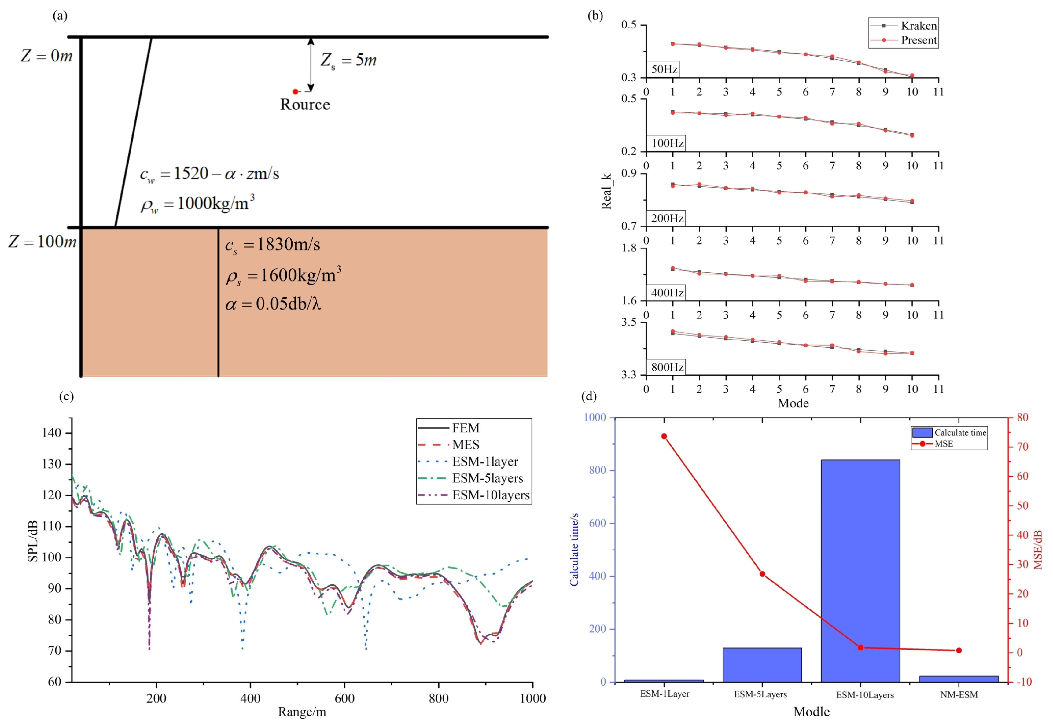
Next, the accuracy of the basis function solution and its application in the equivalent source method are verified. Consider the waveguide environment depicted in Figure 5a, where the water depth is 100 m, the density is 1000 kg/m³, and the sound speed varies from 1520 m/s to 1420 m/s with a negative gradient. The liquid seabed has a density of 1830 kg/m³ and a sound speed of 1600 m/s, with seabed attenuation of 0.05 dB/$\lambda$. First, the accuracy of the eigenvalue computation for the basis function is compared with the eigenvalues obtained from KRAKEN, which serve as a reference standard. Additionally, the acoustic field results from finite element calculations serve as the benchmark.

The comparison of eigenvalue computation accuracy is shown in Figure 5b, where the first ten eigenvalues for several frequencies are presented. The results demonstrate that the eigenvalues calculated in this study are in high agreement with those from KRAKEN. Furthermore, the calculated eigenvalues and eigenfunctions are utilized as basis functions in the equivalent source method and compared with results from traditional equivalent source method in stratified water environments. The traditional equivalent source method employ one layer, five layers, and ten layers water divisions, using consistent methods and the same number of equivalent source points for each model.

Figure 5c presents the one dimensional sound field results at a receiver depth of 50 m. The results demonstrate that the modal equivalent source model closely matches the finite element results, while the traditional equivalent source method only shows good agreement when utilizing ten layers water division. This indicates that vertical stratification in traditional models must achieve a certain level of discretization accuracy to ensure valid results.

Figure 5d compares the traditional equivalent source method with the modal equivalent source model in terms of computational error and time. As the number of vertical layers increases, the computational error of the traditional models decreases, but the computation time increases significantly. For instance, at 100 Hz, the equivalent source distribution interval is 1 m, resulting in system matrix sizes of $3\times 1000$ (3 source groups, 1000 points each) for the single layer model, expanding to $11\times 1000$ and $21\times 1000$ for 5 layers and 10 layers models, respectively. The computation times for the three models were 8 s, 129 s, and 840 s, respectively. However, it should be noted that the average error remains below 2dB only in the 10 layers model. This leads to drastic efficiency degradation. In contrast, the modal equivalent source model avoids water column stratification, maintaining a constant matrix size. The computation time for this model was 23 s, with an average computation error within 2 dB. By introducing new basis functions, this paper reduces the matrix size of the equivalent source method from ${(1+2N_w·N_s)}^2$ to ${\left(2N_s\right)}^2$, thereby improving computational efficiency. Although the basis functions involve higher complexity than free field Green’s functions, the computational time remains marginally higher than the single layer model but overall superior in efficiency.

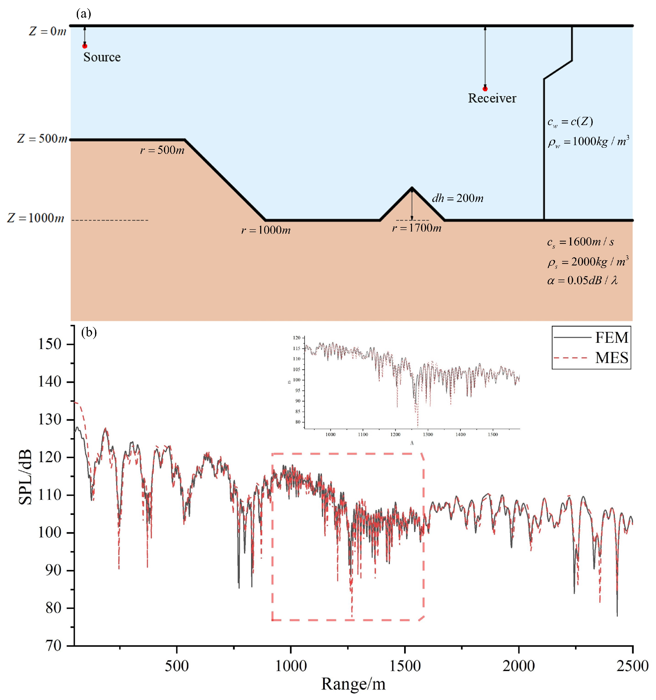
Finally, the applicability of the modal equivalent source model in range dependent waveguide is verified, and the error factors of the model are analyzed. The simulation environment for this case is shown in Figure 6a, where the maximum water depth is 1000 m, with a density of 1000 kg/m³ and a sound speed that decreases from 1520 m/s to 1460 m/s. The seabed has a density of 2000 kg/m³ and a sound speed of 1600 m/s, with seabed attenuation of 0.05 dB/$\lambda$. The source depth is 50 m, and the receiver depth is 300 m. The computed acoustic field results, shown in Figure 6b, are compared against finite element calculation results as the reference. The average error between the two models was 3.2 dB, with FEM requiring a computation time of 16 min 52 s, whereas MES completed in 75 s. The modal equivalent source model exhibits strong agreement with the finite element results, demonstrating its high applicability in more complex waveguide environments. By constructing a set of modes satisfying the semi infinite space condition, the model can compute the acoustic field at any point within the semi infinite domain. Further, by superimposing equivalent sources representing seabed boundaries, it extends to waveguide scenarios with range dependent seabed conditions. Thus, the model requires only a single set of normal modes to compute propagating fields in range dependent environments, eliminating the need for separate modal calculations at different depths.

Based on the theoretical foundation of the modal equivalent source model and the simulation results above, certain errors persist. First, errors primarily arise from the construction of modal basis functions. On one hand, while a semi infinite space theoretically requires an infinite number of modes, practical computations involve a finite set. On the other hand, numerical errors in eigenvalue and eigenfunction calculations contribute additional inaccuracies. These factors manifest as larger errors in Green’s function and acoustic field computations when the distance between equivalent sources and reception points is small. To mitigate this, it is recommended to select a larger equivalent boundary depth and ensure sufficient modal quantities. In this example, the equivalent boundary depth is set to twice the actual maximum seabed depth, with small step sizes adopted for eigenvalue and eigenfunction calculations. Furthermore, errors arise from the impact of the equivalent source distribution on the source strength calculation and sound field computation. Relevant studies (Abawi and Porter [31]) indicate that the distribution of equivalent sources should be based on a quarter wavelength reference distance. However, in practical applications, the optimal distribution differs at various frequencies. In the numerical examples presented in this paper, the optimal distribution of equivalent sources ranges from one fifth to one half of the wavelength. Within the numerical examples, results were computed for numerous different equivalent source point distributions. The distribution yielding the minimum reconstruction error was selected as the final configuration. Subsequent research will further explore the optimal distribution patterns for equivalent sources.

4. Simulation Case Analysis

The ribbed cylinder serves as a typical underwater target structure. Analyzing its radiation and propagation sound field in a range dependent waveguide is essential for underwater target recognition, noise assessment, and design. This study investigates the radiation and propagation sound field of a cylindrical shell in a shallow water waveguide with range dependent variations. The schematic of the cylindrical shell is shown in Figure 7. The cylinder has a diameter of 1270 mm and a length of 3810 mm, with two internal compartments. Each compartment contains seven ribbed rings, each 12.7 mm thick and 50.8 mm wide. The shell thickness is 6.35 mm. The material properties include a Young’s modulus of $7\times {10}^{10}$ N/m², a Poisson’s ratio of 0.3, and a density of 2710 kg/m³. The excitation force, applied at the center of the cylinder, is 10 N.

To ensure the accuracy of the input radiated sound field, the finite element modeling of the target is first described and analyzed. Triangular elements with a maximum element size of one-tenth of the acoustic wavelength discretize the target structure. Triangular elements with a maximum element size of one-sixth of the acoustic wavelength discretize the surrounding fluid domain. The perfectly matched layer (PML) consists of mapped elements with a maximum element size of one-sixth of the acoustic wavelength. Furthermore, grid convergence was verified by computing the result deviation for different element sizes relative to a reference mesh size of one-thirtieth of the acoustic wavelength; the results are presented in

Table 1. Mesh Convergence Comparison Results.

Mesh Size	1/5$\mathit{\lambda }$	1/6$\mathit{\lambda }$	1/10$\mathit{\lambda }$	1/15$\mathit{\lambda }$	1/20$\mathit{\lambda }$
Error	6.9%	2.1%	0.95%	0.42%	0.35%

. The comparison indicates minimal deviation within the given element size range, confirming sufficient convergence. The finite element meshing strategy employed in this study is verified.

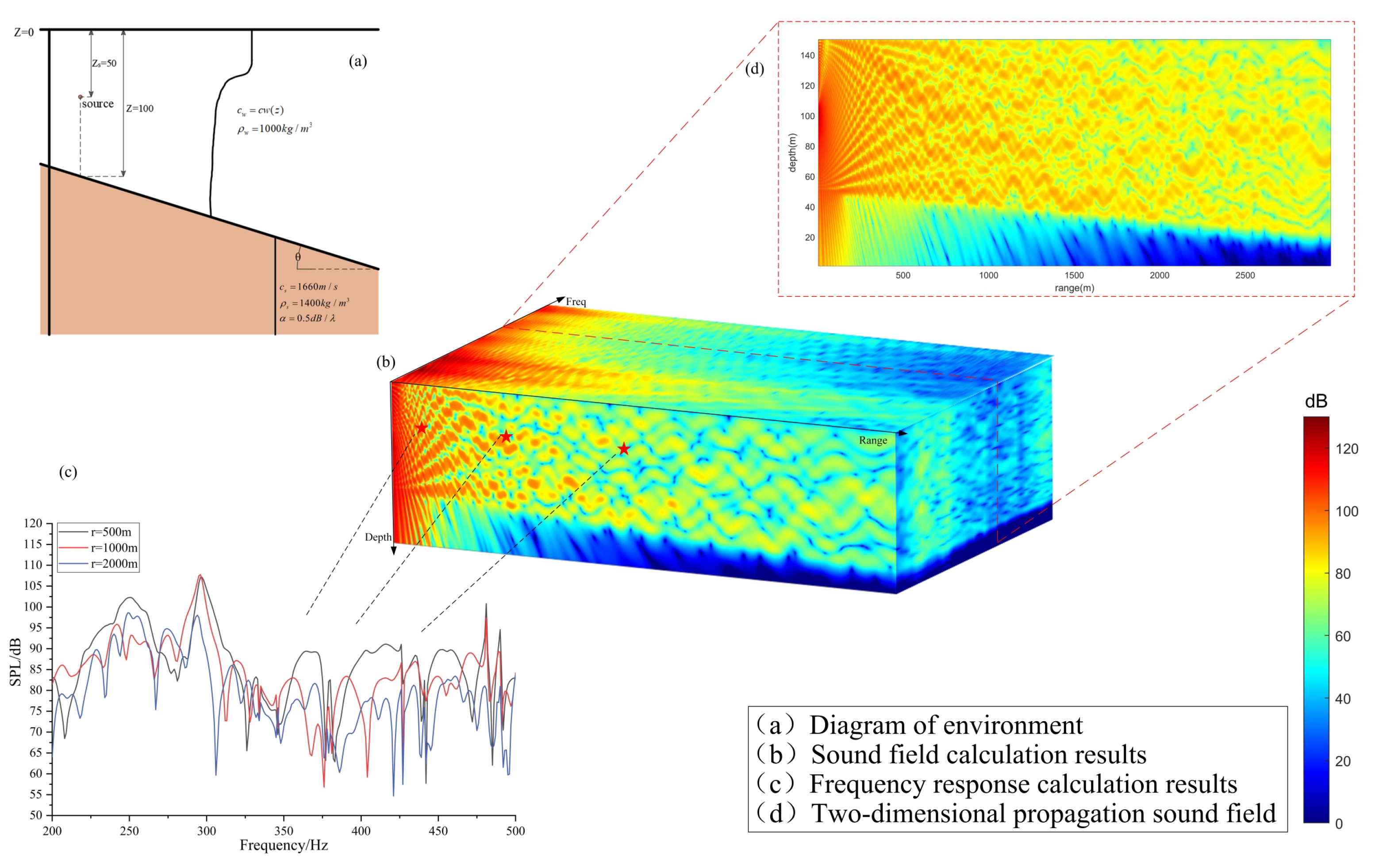
To analyze the effect of the waveguide environment on the radiation and propagation sound field, this paper calculates the sound field of the target using a wedge shaped waveguide as an example (see Figure 8a). In the downward sloping wedge shaped waveguide, the depth of the cylindrical target structure is 50 m, while the water depth at the target location is 100 m. The water density is 1000 kg/m³, and the sound speed decreases with depth in a step like manner (see Figure 8a). The seabed sound speed is 1400 m/s, the seabed density is 1660 kg/m³, the seabed attenuation is 0.5 dB/$\lambda$, and the seabed slope is $tan\alpha =0.01$.

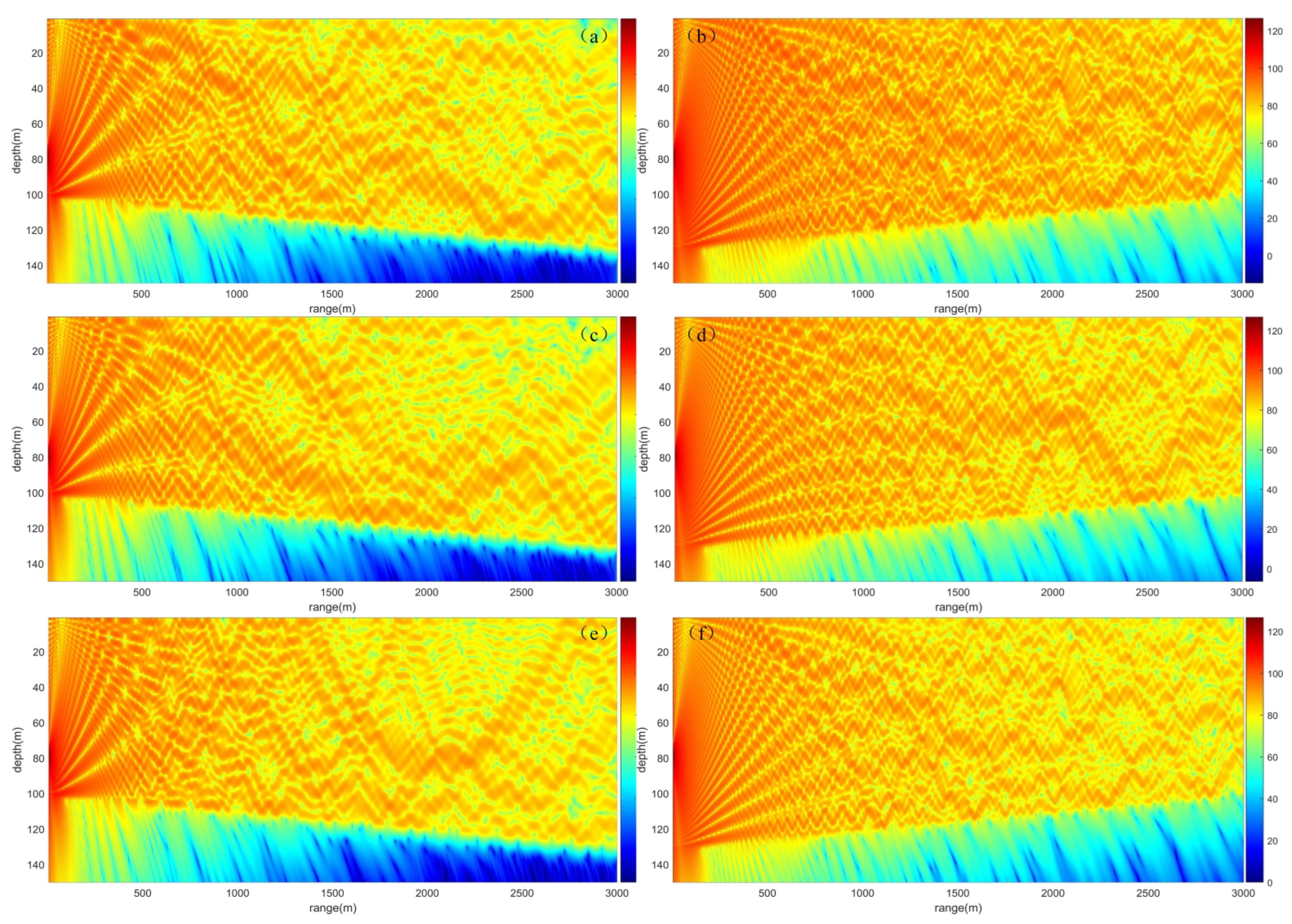
The sound field results are shown in Figure 8, where Figure 8b presents the depth distance frequency results, Figure 8c illustrates the frequency response at positions (50 m, 500 m), (50 m, 1000 m), and (50 m, 2000 m), and Figure 8d provides the depth distance results at selected frequencies. From the energy distribution of the acoustic field in the wedge shaped waveguide environment, it is evident that during sound propagation, multiple reflections between the sea surface and seabed generate distinct interference patterns. As frequency increases, the interference structure of the acoustic field becomes more complex, accompanied by enhanced attenuation. Concurrently, the transmitted acoustic energy through the seabed and its attenuation exhibit an increasing trend. Analysis of the frequency response reveals that as propagation distance grows, the increased number of reflections between the sea surface and seabed introduces greater complexity to the frequency response curves. Furthermore, the characteristics of these curves differ significantly across varying propagation environments. Notably, comparisons of results at different distances and under different environmental conditions demonstrate that local extrema in the frequency response curves consistently correspond to the structural resonance frequencies of the target, such as 209 Hz, 251 Hz, 298 Hz, 378 Hz, and 428 Hz. This indicates that the acoustic field at resonance frequencies is predominantly governed by the target structure itself.

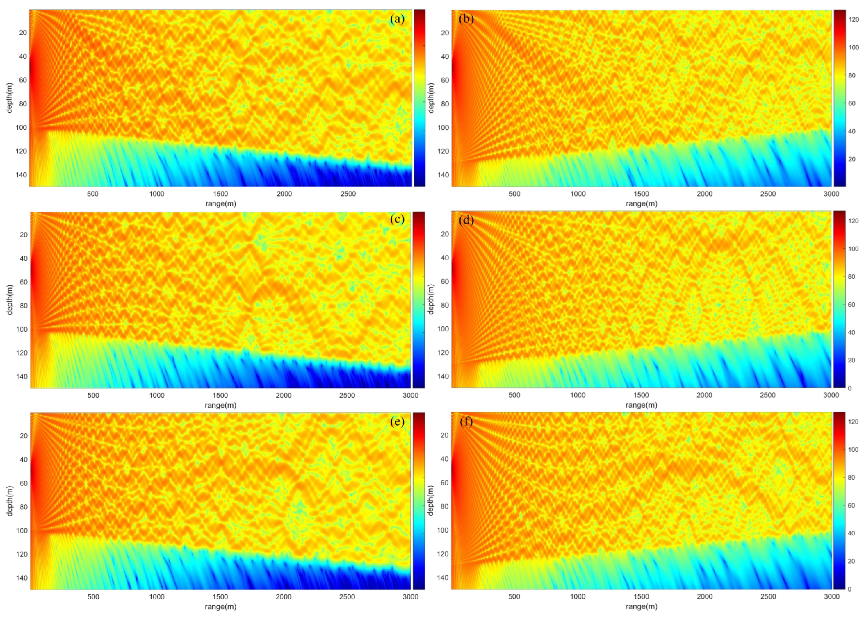
To further illustrate the impact of the waveguide environment on the radiation and propagation sound field, calculations were performed for two cases: a downward sloping wedge shaped waveguide and an upward sloping wedge shaped waveguide, each with different hydrological parameters. The sound speed profile of the water is shown in Figure 9, where, in addition to the existing negative step layer, both negative and positive gradients are considered. For the seabed, a harder seabed is assumed, with a seabed sound speed of 1836 m/s, a seabed density of 2030 kg/m³, and a seabed attenuation of 0.5 dB/$\lambda$. Additionally, the case of a target located at a depth of 80 m is considered.

The acoustic field results at 500 Hz are shown in Figure 10. First, comparisons are made between the results in upward sloping and downward sloping wedge waveguides. Drawing on theories of coupled normal mode and generalized ray theory, in upward sloping waveguides, the real part of each normal mode eigenvalue decreases as water depth shallows. The direction of the real part indicates the propagation direction of the acoustic field. Consequently, for upward sloping scenarios, generalized rays carrying acoustic energy deflect toward regions of increasing water depth. Simultaneously, due to reflections from the sea surface and seabed, as water depth decreases, the horizontal spacing of generalized rays at the same depth along the propagation direction reduces. This compression of acoustic energy during propagation results in denser interference structures. Analogously, for downward sloping waveguides, the real part of each normal mode eigenvalue increases with water depth, causing generalized rays to deflect toward deeper regions. As water depth increases, the horizontal spacing of generalized rays expands along the propagation direction at the same depth, leading to sparser acoustic energy distribution and less densely packed interference structures.

Further comparisons are conducted for acoustic fields under different sound speed profiles. Under identical seabed and sea surface boundary conditions, interference structures exhibit significant variations across sound speed profiles. Near field regions show minimal differences, but discrepancies amplify with propagation distance. Specifically, under negative thermocline conditions, acoustic rays deflect toward lower sound speed regions, causing pronounced downward shifts in interference structures. In contrast, regions with near isospeed profiles exhibit uniform interference patterns. Compared negative and positive gradient conditions, negative gradients induce gradual downward shifts in interference structures with propagation distance, while positive gradients drive upward shifts. In the downward sloping wedge waveguide, increasing water depth and larger sound speed gradients exacerbate structural shifts, whereas the upward sloping case, with decreasing water depth and smaller gradients, yields weaker shifts.

Moreover, results indicate near field consistency across all three sound speed profiles, but divergences emerge progressively with distance. Near field regions, with minimal horizontal seabed variations, show similar outcomes between waveguide types. However, far field regions exhibit marked differences due to sound speed profiles and environmental variations. Notably, upward shifts caused by positive gradients result in slightly higher sound pressure levels (SPL) compared to other profiles. In summary, near field acoustic propagation demonstrates low sensitivity to sound speed profiles, with field structures primarily governed by the target and boundary conditions. Consequently, many models simplify environmental assumptions in near field regions for computational efficiency. However, far field predictions necessitate explicit consideration of sound speed profiles and horizontal waveguide variations.

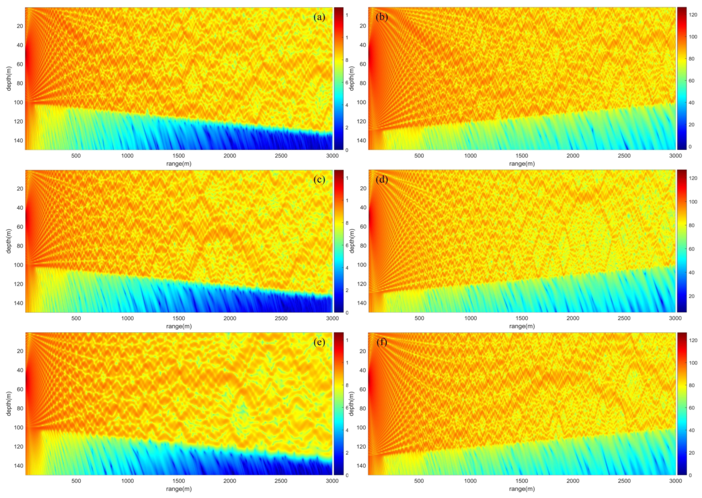
The computed acoustic field results under “hard seabed” conditions are shown in Figure 11. In this scenario, the equivalent seabed reflection coefficient increases significantly, leading to a substantial reduction in acoustic energy transmitted into the seabed and a corresponding rise in energy retained within the waveguide. Consequently, interference structures in the acoustic field become sharper and more pronounced. Similar to soft seabed conditions, sound speed profile induced shifts in interference structures remain observable. Further analyses examine the influence of seabed density, sound speed, and attenuation coefficient on the acoustic field. Results indicate that seabed sound speed and density exert significantly greater impacts on sound propagation than attenuation. In near field regions, acoustic propagation shows insensitivity to seabed attenuation, with consistent results across varying attenuation values. In far field regions, despite similar distribution trends, amplitude differences at specific distances become evident. This suggests that seabed attenuation has a relatively minor overall influence, primarily correlating with propagation distance and frequency effects intensify with longer distances and higher frequencies.

Beyond waveguide conditions, target depth also significantly impacts acoustic radiation and propagation characteristics. Additional analyses compare acoustic fields for varying target depths. For instance, Figure 12 presents results for a target depth of 80 m. When the target is deeper, seabed reflected fields strengthen markedly, with interference structures dominated by direct and seabed reflected paths. Transmitted energy into the seabed also increases. These results demonstrate distinct interference patterns across target depths, where depth influences both direct and reflected fields, with reflections playing a more dominant role. Notably, sound speed profile induced interference shifts persist, but energy concentrates predominantly in the lower half of the water column. Analysis of sound pressure level variations with propagation distance reveals that under positive gradient conditions, sound pressure level no longer exceeds results from negative thermocline or gradient scenarios. This phenomenon becomes more pronounced in downward sloping waveguides, where water depth increases with propagation distance.

Through comparative analyses of varying environmental parameters and target depths, it is evident that acoustic field structures exhibit marked differences under different acoustic environments and target conditions. Among these factors, range dependent waveguide environments and water column sound speed profiles emerge as primary determinants of interference structure characteristics, followed by seabed geological types. Additionally, target depth significantly influences acoustic field outcomes, particularly under specific waveguide environments and seabed parameters, where it markedly alters the properties of seabed reflected fields. Sensitivity to environmental parameters also varies with propagation distance. In near field regions, the water column sound speed profile, seabed attenuation coefficient, and seabed density exert relatively minor impacts on the acoustic field. To enhance computational efficiency, selective omission of certain parameters may be justified. However, in far field regions, the influence of all parameters becomes non negligible. To ensure sufficient accuracy, the combined effects of these parameters must be comprehensively considered.

5. Experimental Application Analysis

This subsection verifies the model through marine experimental data. Our research group conducted sea test in the South China Sea. Field measurements of target-radiated sound fields during sea trials present inherent challenges, particularly in accurately characterizing acoustic emissions from volumetric sources. To address this limitation, a controlled methodology was implemented: transducer-generated simulated radiation signals were transmitted, with the acoustic spectra acquired by monitoring hydrophone serving as equivalent source inputs, enabling focused verification of the Model. 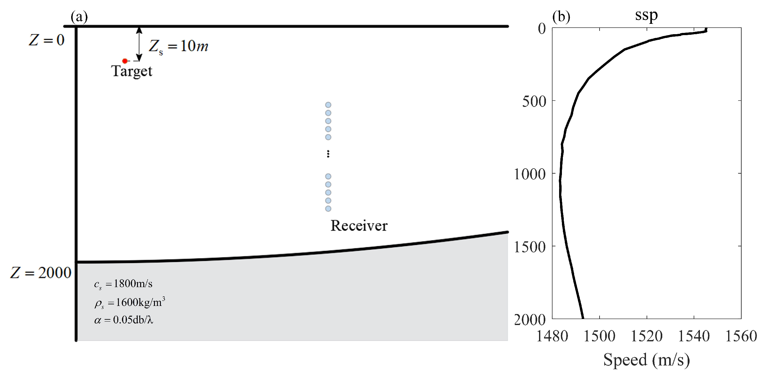Figure 13 illustrates the bathymetric configuration of the test region and associated hydrographic parameters. During the test, a 10 m-deep sound source and a vertical receiving array were deployed. The sound speed profile is shown in Figure 13b, with the seabed featuring a gentle slope reaching 2000 m maximum depth. Seabed parameters were inverted from transmission data with values: $c_b=1800$ m/s, ${\rho }_b=1600$ m/s, $\alpha$ = 0.5 dB/$\lambda$.

The model verification process is divided into the following key steps: Obtain the spectral characteristics of the target radiated source, denoted as $X\left(\omega \right)$, which includes both continuous and discrete spectral components. Based on $X\left(\omega \right)$, the frequency range for the sound field calculation can be determined. In the field tests, the signal collected by the listening devices is processed and used as the source spectrum; Obtain the required parameters for the computational model from the field tests. These parameters are then incorporated into the modal equivalent source model developed in this paper to compute the channel response; Compute the predicted results after channel propagation. The model calculates the sound field response (in the frequency domain) from the sound source to the receiver, denoted as $H\left(\omega \right)$, and couples this with the target’s radiated source characteristics $X\left(\omega \right)$ to predict the target’s radiated sound spectral features; The predicted results are compared with the measured target radiated sound spectral features at the receiver points to verify the model.

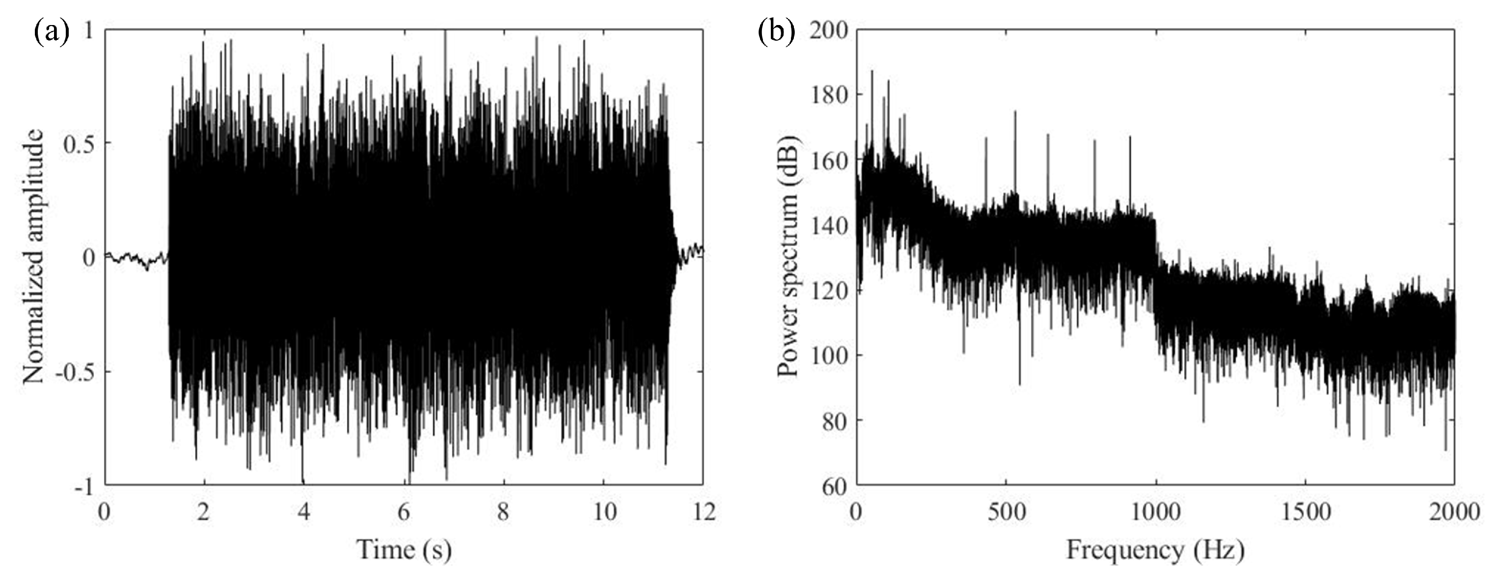
The first step is the acquisition of the source spectrum. The waveform and frequency spectrum characteristics of the signals obtained through listening during the field tests are shown in Figure 14.

The experiment primarily aims to verify the spectral characteristics of the target’s radiated noise. Therefore, the test data must be processed through power spectral estimation to obtain the spectral levels of the target’s radiated sound, including both the line spectrum intensity and continuous spectrum level. The periodogram method is employed to calculate the power spectrum of the target’s radiated signal, following the steps outlined below. First, the data signals are processed using FFT, and then the signal power density within the specified bandwidth $f=f_{\mathrm{b}}-f_{\mathrm{a}}$ is calculated,

$$I_f={\displaystyle \frac{2}{N^{2}f}}\sum _{i=i_a}^{i=i_b}{\left|{\mathrm{P}}_{\mathrm{n}}\left(f_i\right)\right|}^2$$

(26)

where, $f_a={\displaystyle \frac{i_a}{N}}{f}_s$ and $f_b={\displaystyle \frac{i_b}{N}}{f}_s$ represent the lower and upper frequency limits of the bandwidth, respectively. For the continuous spectrum signal of the radiated noise, $f_a$ and $f_b$ correspond to the bandwidth range of 1/3 octave. Finally, the power spectral level of the target’s radiated sound is calculated using the following formula,

$$SPL=10lg\left(I_f\right)-M$$

(27)

In the formula, M represents the sensitivity of the hydrophone. Similarly, the power spectrum of the signal received by the hydrophone is calculated using the same formula. Next, the channel transfer function is determined by combining the obtained waveguide environment parameters and positioning parameters. The predicted received signal power spectrum is then calculated by applying the power spectrum of the transmitted signal. Finally, the predicted power spectrum is compared to the actual received signal power spectrum.

The calculation results for some receiver points are shown in Figure 15. Specifically, Figure 15(a-1–a-3) represent the first position, located 4494 m from the sound source; Figure 15(b-1–b-3) represent the second position, 3069 m from the sound source; and Figure 15(c-1–c-3) represent the third position, 960 m from the sound source. The receiver depths for these positions are 605 m, 995 m, and 1295 m, respectively. The results indicate that the average errors at the three positions are 4.27 dB, 3.53 dB, and 3.59 dB, with average correlation coefficients exceeding 0.9, suggesting a high degree of agreement between the model’s calculated results and the actual received results. The primary source of model error arises from discrepancies between the actual experimental environment and the parameters used in the model’s calculations, including unknown variations in the underwater environment, offsets in the transmitting and receiving positions, and equipment precision. Furthermore, the results indicate that the calculation error for line spectra is significantly higher than that for continuous spectra. This discrepancy is attributed to the propagation characteristics of line spectrum signals and the methods employed in signal processing. In practical ocean engineering applications, analyzing line spectrum signals requires more precise waveguide environmental information. Additionally, such analysis is complicated by interference from ocean ambient noise, making it more challenging. This section primarily verifies the effectiveness of the acoustic field modeling calculations; the overall trend of the calculated results remains consistent with actual received data. These findings demonstrate that the model developed in this paper effectively verifies field test data, showing high reliability and effectiveness.

6. Conclusions

This study overcomes application limitations of the ESM in range-dependent waveguides with depth-dependent acoustic parameters, such as deep-sea environments and polar regions, through the development of a modal equivalent source model. Furthermore, an integrated radiation-propagation computational model has been established through coupling MES with the FEM. Traditional ESM using free-field basis functions have been shown to necessitate vertical waveguide stratification based on depth-varying parameters. Insufficient layering has proven inadequate to resolve vertical parameter discontinuities, compromising accuracy, while excessive layers have yielded computational matrices sized ${(1+2N_w·N_s)}^2$, requiring prohibitive computational cost. This study has employed normal modes as basis functions for the equivalent source method, embedding water column parameter information into these functions. This approach has enabled full-domain modeling of the water column while circumventing stratification-induced issues, reducing the solution matrix size to ${\left(2N_s\right)}^2$ and significantly enhancing computational efficiency. A rapid construction method for normal modes has been developed, leveraging phase function relationships of modal eigenvalues and difference equations for eigenmodes. Furthermore, the theoretical framework and implementation workflow of the integrated model have been established by coupling the FEM-based acoustic radiation model with the MES-based propagation model through their interaction mechanisms. Verification through simulations has demonstrated strong alignment between the integrated model and FEM results (errors < 4 dB), while computation time has been reduced to <1/25th of traditional methods, confirming the model’s precision and efficiency in radiation-propagation field calculations. The model has also been applied to analyze acoustic fields of cylindrical shell in shallow seas, investigating impacts of waveguide variations, sound speed profiles, seabed types, and target depths on interference structures. Results have identified range-dependent waveguides and sound speed profiles as dominant factors shaping interference patterns, with sensitivity varying by propagation distance. Sea trial applications have verified model effectiveness, yielding mean correlation coefficients > 0.9 and mean errors < 5 dB against measured data. Through rigorous verification, this research has confirmed the validity and efficiency of the proposed FE/MES framework, while analyzing key sound field parameters to establish foundations for future applications.

References

1. Wang, S.; Wang, H.; Bian, Z.; Chen, S.; Song, P.; Su, B.; Gao, W. A Robust Direction-of-Arrival (DOA) Estimator for Weak Targets Based on a Dimension-Reduced Matrix Filter with Deep Nulling and Multiple-Measurement-Vector Orthogonal Matching Pursuit. Remote Sens. 2025, 17, 477. [Google Scholar] [CrossRef]
2. Pang, J.; Gao, B. Application of a Randomized Algorithm for Extracting a Shallow Low-Rank Structure in Low-Frequency Reverberation. Remote Sens. 2023, 15, 3648. [Google Scholar] [CrossRef]
3. Chen, L.; Liang, X.; Yi, H. Vibro-acoustic characteristics of cylindrical shells with complex acoustic boundary conditions. Ocean Eng. 2016, 126, 12–21. [Google Scholar] [CrossRef]
4. Jiang, L.; Zou, M.; Huang, H.; Feng, X. Integrated calculation method of acoustic radiation and propagation for floating bodies in shallow water. J. Acoust. Soc. Am. 2018, 143, EL430–EL436. [Google Scholar] [CrossRef] [PubMed]
5. Huang, H.; Zou, M.-S.; Jiang, L.-W. Study on the integrated calculation method of fluid–structure interaction vibration, acoustic radiation, and propagation from an elastic spherical shell in ocean acoustic environments. Ocean Eng. 2019, 177, 29–39. [Google Scholar] [CrossRef]
6. Zhang, L.; Duan, J.-X.; Da, L.-L.; Xu, G.-J.; Sun, X.-H. Vibroacoustic radiation and propagation properties of slender cylindrical shell in uniform shallow sea. Ocean Eng. 2020, 195, 106659. [Google Scholar] [CrossRef]
7. Zhou, Q.; Joseph, P.F. A numerical method for the calculation of dynamic response and acoustic radiation from an underwater structure. J. Sound Vib. 2005, 283, 853–873. [Google Scholar] [CrossRef]
8. Frendi, A.; Maestrello, L.; Ting, L. An efficient model for coupling structural vibrations with acoustic radiation. J. Sound Vib. 1995, 182, 741–757. [Google Scholar] [CrossRef]
9. Duan, J.-X.; Zhang, L.; Da, L.-L.; Sun, X.-H.; Chen, W.-J. A hybrid algorithm of underwater structure vibration and acoustic radiation-propagation in ocean acoustic channel. Int. J. Nav. Archit. Ocean Eng. 2020, 12, 680–690. [Google Scholar] [CrossRef]
10. Pekeris, C.L. Theory of Propagation of Explosive Sound in Shallow Water; Geological Society of America: Tysons, VA, USA, 1948. [Google Scholar]
11. Jensen, F.B.; Kuperman, W.A.; Porter, M.B.; Schmidt, H.; Tolstoy, A. Computational Ocean Acoustics; Springer: Berlin/Heidelberg, Germany, 2011. [Google Scholar]
12. Lim, P.H.; Ozard, J.M. On the underwater acoustic field of a moving point source. I. Range-independent environment. J. Acoust. Soc. Am. 1994, 95, 131–137. [Google Scholar] [CrossRef]
13. Oba, R.M. Probabilistic range dependence in a numerical average underwater acoustic propagation method. J. Acoust. Soc. Am. 1995, 97 (Suppl. S5), 3315. [Google Scholar] [CrossRef]
14. Holland, C.W. Propagation in a waveguide with range-dependent seabed properties. J. Acoust. Soc. Am. 2010, 128, 2596–2609. [Google Scholar] [CrossRef]
15. He, T.; Wang, B.; Mo, S.; Fang, E. Predicting range-dependent underwater sound propagation from structural sources in shallow water using coupled finite element/equivalent source computations. Ocean Eng. 2023, 272, 113904. [Google Scholar] [CrossRef]
16. Zheng, H.; Liu, G.R.; Tao, J.S.; Lam, K.Y. FEM/BEM analysis of diesel piston-slap induced ship hull vibration and underwater noise. Appl. Acoust. 2001, 62, 341–358. [Google Scholar] [CrossRef]
17. Peters, H.; Kinns, R.; Kessissoglou, N. Effects of internal mass distribution and its isolation on the acoustic characteristics of a submerged hull. J. Sound Vib. 2014, 333, 1684–1697. [Google Scholar] [CrossRef]
18. Li, C.; Liu, N.; Su, J.; Hua, H. Vibro-acoustic responses of a coupled propeller-shaft-hull system due to propeller forces. Ocean Eng. 2019, 173, 460–468. [Google Scholar] [CrossRef]
19. Chen, L.; Lian, H.; Pei, Q.; Meng, Z.; Jiang, S.; Dong, H.-W.; Yu, P. FEM-BEM analysis of acoustic interaction with submerged thin-shell structures under seabed reflection conditions. Ocean Eng. 2024, 309, 118554. [Google Scholar] [CrossRef]
20. Zou, M.; Jiang, L.; Liu, S. A transformation of the CVIS method to eliminate the irregular frequency. Eng. Anal. Bound. Elem. 2018, 91, 7–13. [Google Scholar]
21. Zou, M.-S.; Liu, S.-X.; Jiang, L.-W.; Huang, H. A mixed analytical-numerical method for the acoustic radiation of a spherical double shell in the ocean-acoustic environment. Ocean Eng. 2020, 199, 107040. [Google Scholar] [CrossRef]
22. Gao, W.; Lv, Y.; Li, X.; Yu, G.; Wang, H. An integrated calculation model for vibroacoustic radiation and propagation from underwater structures in oceanic acoustic environments. Ocean Eng. 2024, 304, 117682. [Google Scholar] [CrossRef]
23. Gul, S.; Zaidi, S.S.H.; Khan, R.; Wala, A.B. Underwater acoustic channel modeling using BELLHOP ray tracing method. In Proceedings of the 2017 14th International Bhurban Conference on Applied Sciences and Technology (IBCAST), Islamabad, Pakistan, 10–14 January 2017; pp. 665–670. [Google Scholar]
24. Porter, M.B. Beam tracing for two-and three-dimensional problems in ocean acoustics. J. Acoust. Soc. Am. 2019, 146, 2016–2029. [Google Scholar] [CrossRef]
25. Jensen, F.B.; Kuperman, W.A. Sound propagation in a wedge-shaped ocean with a penetrable bottom. J. Acoust. Soc. Am. 1980, 67, 1564–1566. [Google Scholar] [CrossRef]
26. Lin, Y.-T. Three-dimensional boundary fitted parabolic-equation model of underwater sound propagation. J. Acoust. Soc. Am. 2019, 146, 2058–2067. [Google Scholar] [CrossRef] [PubMed]
27. Sturm, F. Leading-order cross term correction of three-dimensional parabolic equation models. J. Acoust. Soc. Am. 2016, 139, 263–270. [Google Scholar] [CrossRef] [PubMed]
28. Preisig, J.C.; Duda, T.F. Coupled acoustic mode propagation through continental-shelf internal solitary waves. IEEE J. Ocean Eng. 1997, 22, 256–269. [Google Scholar] [CrossRef]
29. Athanassoulis, G.A.; Belibassakis, K.A.; Mitsoudis, D.A.; Kampanis, N.A.; Dougalis, V.A. Coupled mode and finite element approximations of underwater sound propagation problems in general stratified environments. J. Comput. Acoust. 2008, 16, 83–116. [Google Scholar] [CrossRef]
30. Tu, H.; Wang, Y.; Yang, C.; Wang, X.; Ma, S.; Xiao, W.; Liu, W. A novel algorithm to solve for an underwater line source sound field based on coupled modes and a spectral method. J. Comput. Phys. 2022, 468, 111478. [Google Scholar] [CrossRef]
31. Abawi, A.T.; Porter, M.B. Propagation in an elastic wedge using the virtual source technique. J. Acoust. Soc. Am. 2007, 121, 1374–1382. [Google Scholar] [CrossRef]
32. He, T.; Mo, S.; Fang, E.; Wang, M.; Zhang, R. Modeling three-dimensional underwater acoustic propagation over multi-layered fluid seabeds using the equivalent source method. J. Acoust. Soc. Am. 2021, 150, 2854–2864. [Google Scholar] [CrossRef]
33. He, T.; Mo, S.; Guo, W.; Fang, E. Modeling propagation in shallow water with the range-dependent sea surfaces and fluid seabeds using the equivalent source method. J. Acoust. Soc. Am. 2021, 149, 997–1011. [Google Scholar] [CrossRef]
34. Junger, M.C. Sound, Structures, and Their Interaction. J. Acoust. Soc. Am. 1987, 82, 1466. [Google Scholar] [CrossRef]
35. Wang, H.; Wang, N.; Gao, D. A Hamiltonian method for finding broadband modal eigenvalues. J. Acoust. Soc. Am. 2012, 131, 1047–1054. [Google Scholar] [CrossRef] [PubMed]
36. Li, X.; Wang, P.; Song, W.; Gao, W. Modal wavenumber estimation by combining physical informed neural network. J. Acoust. Soc. Am. 2023, 153, 2637. [Google Scholar] [CrossRef] [PubMed]
Figure 1. Schematic Diagram of the Principle of Wave Superposition.
Jmse 13 01456 g001
Figure 2. (a) Schematic Diagram of the Traditional Equivalent Source Model; (b) Schematic Diagram of the Modal Equivalent Source Model.
Jmse 13 01456 g002
Figure 3. Flowchart of the Model.
Jmse 13 01456 g003
Figure 4. (a) Schematic Diagram of the Simulation Environment; (b) Comparison of Radiation Directivity Result.
Jmse 13 01456 g004
Figure 5. (a) Schematic Diagram of the Simulation Environment; (b) Comparison of Eigenvalue Calculation Results; (c) Comparison of Acoustic Field Calculation Results; (d) Comparison of Calculation Errors and Computation Time.
Jmse 13 01456 g005
Figure 6. (a) Schematic Diagram of the Simulation Environment; (b) Comparison of Acoustic Field Calculation Results.
Jmse 13 01456 g006
Figure 7. Schematic Diagram of the Cylindrical Target Structure: (a) Model schematic; (b) Dimensional parameters.
Jmse 13 01456 g007
Figure 8. Schematic Diagram of the Downward Sloping Environmental Waveguide Simulation.
Jmse 13 01456 g008
Figure 9. Schematic Diagram of SSP: (a) negative thermocline velocity gradient; (b) negative velocity gradient; (c) positive velocity gradient.
Jmse 13 01456 g009
Figure 10. Comparison of Acoustic Field Calculation Results: (a) Downward Slope Negative Thermocline Velocity Gradient; (b) Upward Slope Negative Thermocline Velocity Gradient; (c) Downward Slope Negative Velocity Gradient; (d) Upward Slope Negative Velocity Gradient; (e) Downward Slope Positive Velocity Gradient; (f) Upward Slope Positive Velocity Gradient.
Jmse 13 01456 g010
Figure 11. Comparison of Acoustic Field Results under Hard Bottom Conditions: (a) Downward Slope Negative Thermocline Velocity Gradient; (b) Upward Slope Negative Thermocline Velocity Gradient; (c) Downward Slope Negative Velocity Gradient; (d) Upward Slope Negative Velocity Gradient; (e) Downward Slope Positive Velocity Gradient; (f) Upward Slope Positive Velocity Gradient.
Jmse 13 01456 g011
Figure 12. Comparison of Acoustic Field Results for Deep Target: (a) Downward Slope Negative Thermocline Velocity Gradient; (b) Upward Slope Negative Thermocline Velocity Gradient; (c) Downward Slope Negative Velocity Gradient; (d) Upward Slope Negative Velocity Gradient; (e) Downward Slope Positive Velocity Gradient; (f) Upward Slope Positive Velocity Gradient.
Jmse 13 01456 g012
Figure 13. Schematic diagram of the test environment: (a) Schematic diagram of waveguide; (b) SSP.
Jmse 13 01456 g013
Figure 14. (a) Signal Time Domain Waveform; (b) Signal Power spectrum.
Jmse 13 01456 g014
Figure 15. Comparison of Model Results: (a) is the first station position, (b) is the second station position, and (c) is the third station position; 1 is the first reception depth, 2 is the second reception depth, and 3 is the third reception depth.
Jmse 13 01456 g015