Author Contributions
Conceptualization, A.B., J.K., H.S. and Y.C.L.; Methodology, A.B., J.K., S.J.S.H. and Y.C.L.; Software, A.B., J.K. and V.K.; Validation, A.B.; Investigation, A.B. and J.K.; Resources, A.B., V.K. and Y.C.L.; Data curation, A.B., J.K., S.J.S.H., H.S. and Y.C.L.; Writing—original draft, A.B.; Visualization, A.B. and J.K.; Supervision, Y.C.L.; Funding acquisition, A.B., J.K., V.K. and Y.C.L. All authors have read and agreed to the published version of the manuscript.
Figure 1.
Flowchart of the hydrodynamic and sediment transport coupling procedure at each time step of the scour modelling.
Figure 1.
Flowchart of the hydrodynamic and sediment transport coupling procedure at each time step of the scour modelling.
Figure 2.
The results of the flow field modelling adjacent to an AR at (
a)
= 0.06 cm, (
b)
= 0.10 cm, (
c)
= 0.15 cm on the symmetry plane compared with experimental and numerical results extracted from Wang et al. [
16] and Yang et al. [
45].
Figure 2.
The results of the flow field modelling adjacent to an AR at (
a)
= 0.06 cm, (
b)
= 0.10 cm, (
c)
= 0.15 cm on the symmetry plane compared with experimental and numerical results extracted from Wang et al. [
16] and Yang et al. [
45].
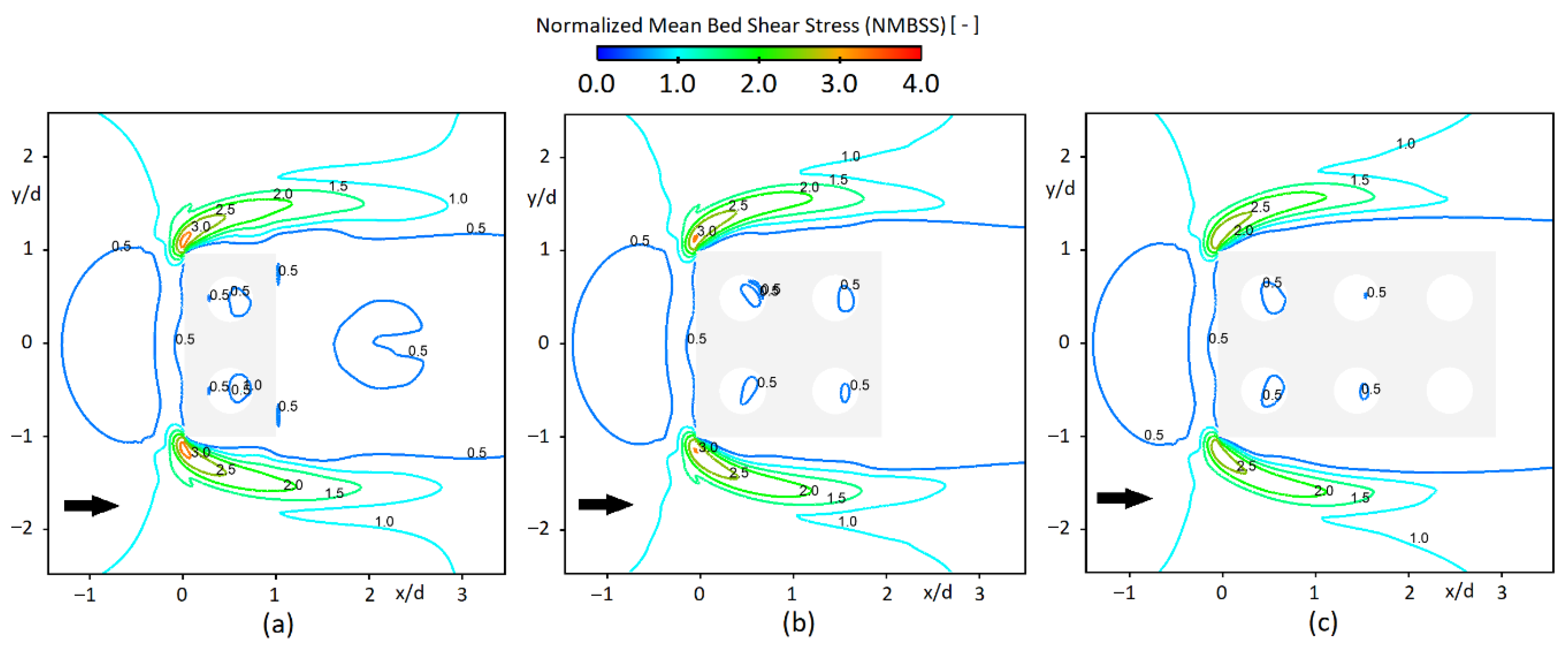
Figure 3.
NMBSS contours of numerical modelling.
Figure 3.
NMBSS contours of numerical modelling.
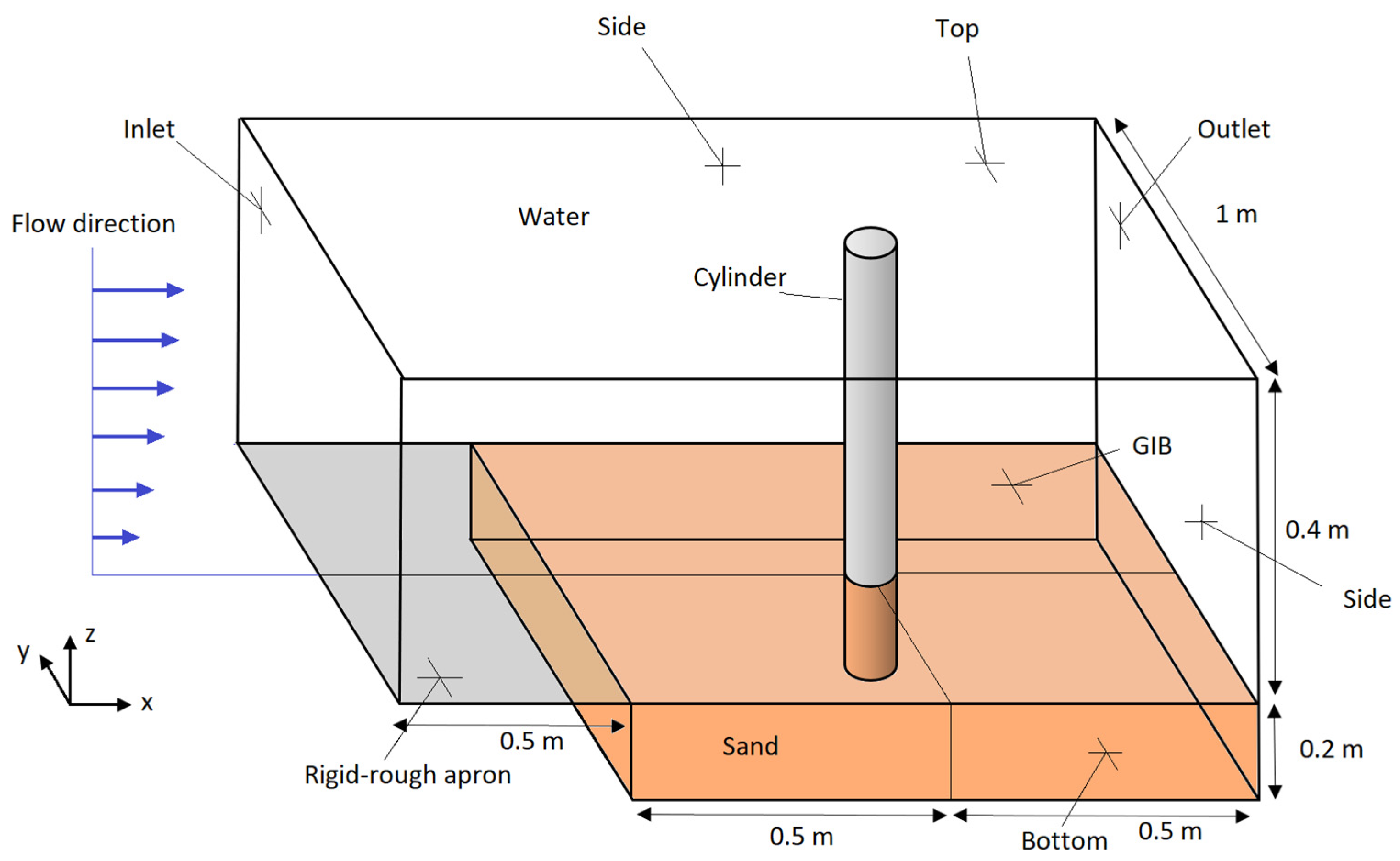
Figure 4.
Computational domain for modelling of scour around circular cylinder.
Figure 4.
Computational domain for modelling of scour around circular cylinder.
Figure 5.
(
a) Simulated local scour at t = 10 min, (
b) Progression of maximum local scour depth over time during the first 10 min of the simulation, compared with experimental results extracted from Roulund et al. [
41].
Figure 5.
(
a) Simulated local scour at t = 10 min, (
b) Progression of maximum local scour depth over time during the first 10 min of the simulation, compared with experimental results extracted from Roulund et al. [
41].
Figure 6.
(a) An RC deployed in the waters of Torbay; (b) Schematic of the geometric characteristics of the RC designed by ARC Marine; (c,d) RCs with 90° and 45° orientation angles to the flow, each with a side length of D = 1.5 m; (e–g) Arrangement of groups of two, four, and six RCs, each with a side length of D = 0.75 m; (h–j) A group of ten RCs with different arrangements of the top four cubes in the front, middle, and back, each with a side length of D = 0.75 m.
Figure 7.
Generated mesh near the RC with 90° orientation, showing local mesh refinement in the region of interest: (a) horizontal plane at Z = 0.75 m, (b) vertical plane at Y = 0 m.
Figure 7.
Generated mesh near the RC with 90° orientation, showing local mesh refinement in the region of interest: (a) horizontal plane at Z = 0.75 m, (b) vertical plane at Y = 0 m.
Figure 8.
Flow field contours at different horizontal plane Z = 0.375 m, Z = 0.75 m, and Z = 1.125 m for a single RC with (a–c) 90° and (d–f) 45° orientation angle to the flow, respectively.
Figure 8.
Flow field contours at different horizontal plane Z = 0.375 m, Z = 0.75 m, and Z = 1.125 m for a single RC with (a–c) 90° and (d–f) 45° orientation angle to the flow, respectively.
Figure 9.
Flow field contours at different vertical plane Y = 0 m, and Y = 0.375 m for a single RC with (a,b) 90° and (c,d) 45° orientation angle to the flow, respectively.
Figure 9.
Flow field contours at different vertical plane Y = 0 m, and Y = 0.375 m for a single RC with (a,b) 90° and (c,d) 45° orientation angle to the flow, respectively.
Figure 10.
NMBSS contours for single RCs with different orientation angles to the flow (Top) 45°, and (Bottom) 90°.
Figure 10.
NMBSS contours for single RCs with different orientation angles to the flow (Top) 45°, and (Bottom) 90°.
Figure 11.
Flow field at a horizontal plane (Z = 0.375 m) for the arrangements of (a) two, (b) four, and (c) six RCs.
Figure 11.
Flow field at a horizontal plane (Z = 0.375 m) for the arrangements of (a) two, (b) four, and (c) six RCs.
Figure 12.
Flow field at vertical planes Y = 0 m and Y = 0.375 m for the arrangements of (a,b) two, (c,d) four, and (e,f) six RCs, respectively.
Figure 12.
Flow field at vertical planes Y = 0 m and Y = 0.375 m for the arrangements of (a,b) two, (c,d) four, and (e,f) six RCs, respectively.
Figure 13.
NMBSS contours for arrangements of (a) two, (b) four, and (c) six RCs.
Figure 13.
NMBSS contours for arrangements of (a) two, (b) four, and (c) six RCs.
Figure 14.
Flow field contours for a group of ten RCs with different arrangements of the top four cubes; (a,c,e) for front, middle, and back arrangements at Z = 0.375 m, respectively; and (b,d,f) for front, middle, and back arrangements at Z = 1.125 m, respectively.
Figure 14.
Flow field contours for a group of ten RCs with different arrangements of the top four cubes; (a,c,e) for front, middle, and back arrangements at Z = 0.375 m, respectively; and (b,d,f) for front, middle, and back arrangements at Z = 1.125 m, respectively.
Figure 15.
Flow field contours for a group of ten RCs with different arrangements of the top four cubes; (a,c,e) for front, middle, and back arrangements at Y = 0 m, respectively; and (b,d,f) for front, middle, and back arrangements at Y = 0.375 m, respectively.
Figure 15.
Flow field contours for a group of ten RCs with different arrangements of the top four cubes; (a,c,e) for front, middle, and back arrangements at Y = 0 m, respectively; and (b,d,f) for front, middle, and back arrangements at Y = 0.375 m, respectively.
Figure 16.
NMBSS contours for a group of ten RCs with different arrangements of the top four cubes in (a) front, (b) middle, and (c) back.
Figure 16.
NMBSS contours for a group of ten RCs with different arrangements of the top four cubes in (a) front, (b) middle, and (c) back.
Figure 17.
Computational domain for modelling of scour around RC.
Figure 17.
Computational domain for modelling of scour around RC.
Figure 18.
Time evolution of maximum scour depth and deposition height near the RC.
Figure 18.
Time evolution of maximum scour depth and deposition height near the RC.
Figure 19.
Water-sand interface displacement contours for (a) = 0.2 m/s and (b) = 0.4 m/s at t = 10 min.
Figure 19.
Water-sand interface displacement contours for (a) = 0.2 m/s and (b) = 0.4 m/s at t = 10 min.
Table 1.
Applied boundary condition for model validation against the experimental test conducted by Wang et al. [
16].
Table 1.
Applied boundary condition for model validation against the experimental test conducted by Wang et al. [
16].
| Boundaries | Sides | Top | Bed | Inlet | Outlet | AR |
|---|
| Velocity () | no-slip | Slip | no-slip | fixedValue | inletOutlet | no-slip |
| Pressure ()
| zeroGradient | Slip | zeroGradient | zeroGradient | fixedValue | zeroGradient |
| Turbulent ki-netic energy () | kqRWallFunction | Slip | kqRWallFunction | fixedValue | inletOutlet | kqRWallFunction |
| Specific turbu-lent dissipation rate () | omegaWallFunction | Slip | omegaWallFunction | fixedValue | inletOutlet | omegaWallFunction |
| Kinematic tur-bulent viscosity () | nutkWallFunction | Slip | nutkWallFunction | calculated | calculated | kqRWallFunction |
Table 2.
Details of experiment test by Sadeque et al. [
46].
Table 2.
Details of experiment test by Sadeque et al. [
46].
| Water Depth () [m] | Discharge [L/s] | Mean Velocity () [m/s] | Cylinder Reynolds Number [-] |
|---|
| 0.220 | 50 | 0.186 | 21,000 |
Table 3.
Applied boundary condition for model validation against the experiment conducted by Sadeque et al. [
46].
Table 3.
Applied boundary condition for model validation against the experiment conducted by Sadeque et al. [
46].
| Boundaries | Sides | Top | Bed | Inlet | Outlet | Cylinder |
|---|
| Velocity () | Symmetry | Slip | no-slip | fixedValue | inletOutlet | no-slip |
| Pressure (
)
| Symmetry | Slip | zeroGradient | zeroGradient | fixedValue | zeroGradient |
| Turbulent kinetic energy () | Symmetry | Slip | kqRWallFunction | fixedValue | inletOutlet | kqRWallFunction |
| Specific turbulent dissipation rate () | Symmetry | Slip | omegaWallFunction | fixedValue | inletOutlet | omegaWallFunction |
| Kinematic turbu-lent viscosity () | Symmetry | Slip | nutkWallFunction | calculated | calculated | kqRWallFunction |
Table 4.
Applied boundary condition for model validation against experimental data obtained by Roulund et al. [
41].
Table 4.
Applied boundary condition for model validation against experimental data obtained by Roulund et al. [
41].
| Boundaries | Sides | Top | GIB/Rigid-Rough Apron | Inlet | Outlet | Pile |
|---|
| Velocity () | Symmetry | Slip | no-slip | fixedValue | inletOutlet | no-slip |
| Pressure ()
| Symmetry | Slip | zeroGradient | zeroGradient | fixedValue | zeroGradient |
| Turbulent kinetic energy () | Symmetry | Slip | kqRWallFunction | fixedValue | inletOutlet | kqRWallFunction |
| Specific turbulent dissipation rate () | Symmetry | Slip | omegaWallFunction | fixedValue | inletOutlet | omegaWallFunction |
| Kinematic turbu-lent viscosity () | Symmetry | Slip | nutkRoughWallFunction | calculated | calculated | kqRWallFunction |
Table 5.
Applied boundary condition for modelling flow behaviour around RCs.
Table 5.
Applied boundary condition for modelling flow behaviour around RCs.
| Boundaries | Sym | Top | Bed | Inlet | Outlet | RC |
|---|
| Velocityb () | symmetry | Slip | no-slip | fixedValue | inletOutlet | no-slip |
| Pressure ()
| symmetry | Slip | zeroGradient | zeroGradient | fixedValue | zeroGradient |
| Turbulent kinetic energy () | symmetry | Slip | kqRWallFunction | fixedValue | inletOutlet | kqRWallFunction |
| Specific turbulent dissipation rate () | symmetry | Slip | omegaWallFunction | fixedValue | inletOutlet | omegaWallFunction |
| Kinematic turbu-lent viscosity () | symmetry | Slip | nutkRoughWallFunction | calculated | calculated | nutkRoughWallFunction |
Table 6.
Generated meshes for mesh dependency study.
Table 6.
Generated meshes for mesh dependency study.
| Name | Mesh Size | Background Mesh Size [] | Volume of Upwelling Region [] |
|---|
| Coarse | 5.4 × | 0.3 × 0.3 | 5.844 |
| Medium | 6.9 × | 0.25 × 0.25 | 6.088 |
| Fine | 8.8 × | 0.2 × 0.2 | 6.152 |
Table 7.
Magnitude of volume of upwelling and wake regions for single RCs with 90° and 45° orientation angles to the flow.
Table 7.
Magnitude of volume of upwelling and wake regions for single RCs with 90° and 45° orientation angles to the flow.
| Orientation Angle to the Flow | Volume of Upwelling Region [] | Volume of Wake Region [] |
|---|
| Single cube—90° | 6.152 | 3.135 |
| Single cube—45° | 11.172 | 4.668 |
Table 8.
Magnitude of volume of upwelling and wake regions for the arrangement of a group of two, four, and six RCs.
Table 8.
Magnitude of volume of upwelling and wake regions for the arrangement of a group of two, four, and six RCs.
| Group of RCs | RC Volumes | Volume of Upwelling Region [] | Dimensionless
Volume of Upwelling | Volume of Wake Region [] | Dimensionless
Volume of Wake |
|---|
| Two | 0.48 | 3.585 | 7.469 | 1.460 | 3.042 |
| Four | 0.96 | 3.164 | 3.296 | 1.175 | 1.225 |
| Six | 1.44 | 3.208 | 2.228 | 1.239 | 0.860 |
Table 9.
Magnitude of volume of upwelling and wake regions for a group of ten RCs with different arrangements of top four cubes in (a) front, (b) middle, and (c) back.
Table 9.
Magnitude of volume of upwelling and wake regions for a group of ten RCs with different arrangements of top four cubes in (a) front, (b) middle, and (c) back.
| Group of Ten RCs | Volume of Upwelling Region [] | Volume of Wake Region [] |
|---|
| The top four in the front | 6.702 | 2.725 |
| The top four in the middle | 6.723 | 2.460 |
| The top four in the back | 7.149 | 2.616 |
Table 10.
The hydro-morphodynamic model results after 10 min of simulation.
Table 10.
The hydro-morphodynamic model results after 10 min of simulation.
| Mean Flow Speed | RC Reynolds Number [-] | Undisturbed Shields Parameter [-] | Max. Scour Depth [mm] | Max. Deposition Height [mm] |
|---|
| U = 0.2 (m/s) | | 0.015 | 6.8 | 2.6 |
| U = 0.4 (m/s) | | 0.06 | 63.9 | 37.2 |


