Drift Characteristics and Predictive Modeling of Life Rafts in Island and Reef Waters

Abstract

Accurate prediction of drifting trajectories is essential for improving the operational efficiency of maritime search and rescue (SAR), particularly within the complex geomorphological settings of island and reef regions, such as those in the South China Sea. This study investigates the drift characteristics of life rafts under varying loading conditions across both open-sea and island–reef regions. Comprehensive field experiments were conducted over 15 days in the waters around the Wanshan Archipelago, using advanced instruments to collect wind, current, and drift trajectory data. Based on these observations, two models—the AP98 leeway model and a BP neural network model—were developed and validated. The results show that the AP98 model performs better in open-sea conditions, whereas the BP neural network provides more accurate predictions in island and reef areas with complex environmental factors. A Monte Carlo simulation was also integrated to enhance the robustness of drift area predictions. These findings offer valuable insights into life raft drift behavior in complex marine environments and provide technical support for improving SAR operations in island–reef regions.

1. Introduction

The accelerated growth of global trade has considerably intensified maritime operations, resulting in a marked increase in maritime accidents. These incidents often lead to substantial economic losses, loss of human lives, and severe environmental damage. In China, the burgeoning maritime economy has been accompanied by a corresponding rise in maritime emergencies. To mitigate these risks, efficient search and rescue (SAR) operations are crucial, requiring the integration of accurate, timely information and reliable forecasts of sea conditions. This need is particularly pronounced in regions such as the South China Sea, which is characterized by its complex geography, including numerous islands and reefs, thereby posing significant challenges. Accurately representing the hydrostatic and stability behavior of drifting maritime targets under such complex conditions requires precise modeling techniques. Zhang and Xie [1] proposed a force-oriented finite element method for computing statical stability curves of floating bodies with arbitrary configurations. Their method achieves high accuracy while being insensitive to mesh patterns, which is particularly beneficial for modeling irregularly shaped floating objects in complex marine environments such as island and reef waters. The development and application of precise drift prediction models are essential for enhancing SAR operational efficiency and achieving successful outcomes in maritime emergencies [2].

The study of maritime distress drift prediction has a history spanning several decades. One of the earliest foundational studies was conducted by Pingree in 1944, who investigated lifeboat movement and introduced the “Forethoughts on Rubber Rafts” theory [3]. With the advancement of computer technology in the 1970s, technological advancements significantly enhanced drift prediction models, leading to higher rescue success rates. Various nations subsequently developed their drift prediction systems, including Canada’s CANSARP [4], and the United States’ SARMAP [5].

Despite these technological strides, uncertainties continue to challenge maritime search and rescue (SAR) operations, prompting extensive academic research. Shi et al. [6] introduced a model for evaluating SAR capabilities, while Xiong et al. [7] proposed a framework to optimize resource allocation in SAR planning, thereby improving the efficiency of emergency responses. Vandenbulcke et al. [8] explored ensemble methods for predicting buoy trajectories, and Melsom et al. [9] utilized ensemble ocean circulation models to forecast buoy drift, demonstrating the practical utility of ensemble prediction techniques.

Drift studies require a comprehensive analysis of various environmental factors that influence target movement [10,11]. With technological advancements, sensor-equipped buoys have become indispensable tools for data collection in marine experiments [12]. Furthermore, experimental facilities such as water tanks, wind tunnels, and high-frequency radar systems have substantially enhanced the efficiency and accuracy of drift research [13,14,15,16].

Breivik and Allen [2] utilized a stochastic trajectory method to predict lifeboat drift, incorporating uncertainties in wind and current conditions, thereby improving the accuracy of search operations. Burciu and Grabski [17] established a reliability function for lifeboats based on experimental data obtained under different loading and operational conditions. Likewise, Brushett et al. [18] utilized a Lagrangian particle trajectory approach to predict the drift patterns of lifeboats in the Pacific Ocean, facilitating more accurate delineation of search areas.

In the study of drift prediction for persons-in-the-water, Tu et al. [19] conducted field experiments and Monte Carlo simulations in the South China Sea to examine the drift behavior of dummy buoys with horizontal and vertical postures. Their research focused on developing drift models for both vertical and horizontal postures. The results demonstrated that the dynamic drift model outperformed the AP98 leeway drift model in accurately estimating the trajectories of individuals in a vertical posture. Furthermore, it was observed that individuals floating in a vertical posture experienced shorter drift distances compared to those in a horizontal posture. Experimental studies such as Lyu et al. [20] further complement this understanding by analyzing vertical entry of tandem spheres, showing how water-entry dynamics—such as splash, cavity formation, and wake interaction—can significantly affect post-entry motion and drag forces, which are critical factors for modeling vertical PIWs or falling debris.

Regarding the calibration of drift parameters for persons-in-the-water, Allen et al. [21] refined the wind-induced drift coefficient for persons overboard and conducted field experiments to measure the drift velocities of five representative objects. Their findings provided valuable insights into the influence of wind on drift.

In the field of vessel drift prediction, Ni et al. [22] developed a comprehensive vessel drift prediction model that systematically analyzed and quantified uncertainties associated with vessel drift, identifying key sources of uncertainty within the search area. Zhu et al. [23] performed a comprehensive analysis of wind-driven drift behaviors exhibited by representative Chinese fishing vessels and assessed the performance of various drift prediction models. Their field experiments and comparative analysis demonstrated that the AP98 leeway drift model exhibited the highest consistency with observational data. Compared to physically based dynamic drift models, the performance of the AP98 leeway model has been shown to vary with environmental conditions and the physical characteristics of the drifting object. Tu et al. [24] assessed drift predictions for persons-in-the-water (PIWs) and found that dynamic models generally outperformed the AP98 formulation for vertically oriented PIWs, whereas both models yielded comparable accuracy for horizontally oriented targets. In a controlled field experiment conducted in the South China Sea, Mu et al. [25] calibrated both AP98 and dynamic drift models using observations of floating debris. Their comparative simulations indicated that the dynamic model more accurately represented current-dominated drift behavior but was less sensitive to wind-induced crosswind effects. In contrast, the AP98 model more effectively captured directional variability due to wind forcing, though it exhibited greater positional errors under current–wind misalignment. The AP98 leeway model relies on empirically derived “downwind” and “crosswind” coefficients—obtained from extensive field measurements—to decompose wind forcing into orthogonal components through linear operations. This method enhances its ability to capture wind-induced directional variability, especially under wind-dominated or mixed wind–current conditions. However, in scenarios where currents overwhelmingly dominate, physically based dynamic models tend to achieve higher accuracy.

Regarding the calibration of vessel drift parameters, Brushett et al. [26] conducted field studies to analyze the drift characteristics of vessels around tropical Pacific islands and derived drift coefficients, thereby improving the accuracy of search-and-rescue prediction models. Their methodology incorporated direct measurements from current meters deployed on or near the target vessels, along with estimations of current velocity obtained from nearby vessels or floating objects, to infer the yaw coefficients of the studied vessels.

Furthermore, Meng et al. [27] carried out four comprehensive drift experiments on a widely used 20 m-long fishing vessel in the northern region of the South China Sea. Based on the collected data, they established the drift characteristics specific to this vessel type, contributing to a more precise understanding of its drift behavior.

The rapid advancement of artificial intelligence (AI) technologies, supported by increased computational power, has enabled more effective analysis of large-scale datasets, pattern recognition, and prediction of complex outcomes. These capabilities have garnered significant attention across disciplines. For instance, Shahiduzzaman et al. [28] evaluated various machine learning algorithms for renewable energy forecasting, while Aggogeri et al. [29] applied artificial neural networks (ANNs) enhanced with genetic algorithms for robotic arm control, reducing manual configuration and improving accuracy. Among the various application areas of AI, maritime navigation has increasingly adopted machine learning techniques to improve safety and efficiency. In particular, neural network models–a prominent class of machine learning algorithms–have demonstrated considerable potential in addressing complex prediction problems. This potential is largely attributed to their superior nonlinear mapping capabilities and robust self-learning mechanisms. As a result, neural networks are increasingly regarded as a promising and effective approach for improving the accuracy and reliability of maritime drift trajectory predictions.

Beyond conventional optimization techniques, recent advancements have highlighted the efficacy of nature-inspired algorithms—such as Particle Swarm Optimization (PSO), Ant Colony Optimization (ACO), Differential Evolution (DE), and Genetic Algorithms (GAs)—in enhancing the performance of artificial intelligence (AI) models. Sharafati et al. [30] employed these evolutionary algorithms to optimize the internal parameters of an Adaptive Neuro-Fuzzy Inference System (ANFIS) for the prediction of wave-induced scour depth around submarine pipelines. Their results indicated that the hybrid ANFIS-PSO model exhibited superior predictive accuracy under both live-bed and clear-water conditions, outperforming not only conventional ANFIS models but also other contemporary approaches. Moreover, the study incorporated Monte Carlo simulations to quantify the uncertainty associated with model predictions. In a related study, Sharafati et al. [31] further substantiated the utility of hybrid ANFIS models, optimized via nature-inspired algorithms, for estimating scour depth downstream of sluice gates. These investigations collectively underscore the potential of evolutionary optimization techniques—particularly PSO—in improving AI model performance in complex, nonlinear hydraulic contexts, thereby presenting a robust alternative to traditional empirical formulations and standalone AI methodologies.

The field of maritime drift prediction continues to face several critical challenges that warrant further investigation:

1.

While Chinese researchers have extensively examined the drift characteristics of typical maritime targets, most existing studies have focused on open-sea conditions. Drift behaviors in island and reef waters, however, remain comparatively underexplored. To address this gap, the present study investigates target drift within these more complex marine settings, emphasizing their unique dynamic characteristics.

2.

Although traditional approaches such as the AP98 model and dynamic drift models remain widely used in maritime drift prediction, the explosive growth in data and increasing complexity of marine environments have exposed their limitations, particularly in large-scale data processing. In response, this study incorporates machine learning techniques—specifically, a BP neural network model—to enhance predictive performance. The model is rigorously evaluated for its effectiveness in forecasting maritime target drift, aiming to improve both accuracy and adaptability in complex marine conditions.

2. Theoretical Models and Methods

2.1. AP98 Leeway Model

The AP98 leeway model, originally proposed by Allan and Plourde [32], is a semi-empirical numerical model based on field experiments and regression analysis. It postulates that the drift velocity component caused by currents is equivalent to the surface current velocity. For most drifting objects smaller than 30 m in length, wave-induced drift forces decay rapidly as the dominant wavelength increases and can be neglected in comparison to wind-induced forces. This conclusion is supported by field experiments and theoretical analysis in th work of Breivik et al. [33]. This model expresses the total drift velocity $\overrightarrow{V_0}$ as the vector summation of the current-driven component $\overrightarrow{V_{F-c}}$ and the wind-induced drift $\overrightarrow{L}$.

$$\overrightarrow{V_0}=\overrightarrow{V_{F-c}}+\overrightarrow{L}=\overrightarrow{V_c}+\overrightarrow{L}$$

(1)

where $\overrightarrow{V_c}$ denotes the surface current velocity. The model explicitly equates the current-induced drift component $\overrightarrow{V_{F-c}}$ to the surface current speed $\overrightarrow{V_c}$.

A distinctive feature of the AP98 leeway model is its incorporation of a leeway angle, which quantifies the angular deviation between wind direction and resultant drift trajectory. The wind-induced drift vector resolves into two components: downwind drift (DWL) parallel to wind direction, and crosswind drift (CWL) perpendicular to it. The model further specifies directional variants, designating leftward deflection as negative crosswind drift (–CWL) and rightward deflection as positive crosswind drift (+CWL) relative to the wind vector.

The original AP98 leeway model exhibited limitations in characterizing shift angle variations under low wind speed conditions. To address this constraint, Allen [34] conducted methodological refinements through the derivation of an enhanced governing equation for wind-induced drift dynamics. Their model analytically decomposes the drift velocity resulting from wind forcing into two perpendicular components: downwind (DWL) and crosswind (CWL) velocities, each associated with corresponding directional probabilities, as illustrated in Figure 1. The researchers further established equivalent probability distributions for leftward (–CWL) and rightward (+CWL) crosswind components. Subsequently, Breivik et al. [33] advanced the theoretical framework through rigorous parameterization, formally defining leeway as the resultant displacement characteristics of objects subject to wind forcing at 10 m elevation and subsurface current effects between a 0.3 and 1 m depth. This conceptual framework is mathematically expressed as

$$\left\{\begin{array}{c}{L}_d=a_d{V}_w+b_d+{\epsilon }_d\left(\mathit{DWL}\right)\hfill \\ L_{c+}=a_{c+}{V}_w+b_{c+}+{\epsilon }_{c+}(+\mathit{CWL})\hfill \\ L_{c-}=a_{c-}{V}_w+b_{c-}+{\epsilon }_{c-}(-\mathit{CWL})\hfill \end{array}\right.$$

(2)

where $L_d$ denotes the drift velocity due to wind influence in the downwind direction, while $L_{c+}$ and $L_{c-}$ correspond to drift components orthogonal to the wind direction, oriented to the right and left, respectively. The wind speed measured at 10 m above sea surface is denoted by $V_w$. The fitting coefficients are represented by $a_d$, $a_{c+}$, $a_{c-}$, $b_d$, $b_{c+}$, and $b_{c-}$, whereas the associated error terms are denoted as ${\epsilon }_d$, ${\epsilon }_{c+}$, and ${\epsilon }_{c-}$.

2.2. BP Neural Networks Model

Backpropagation (BP) neural networks, as a prominent class of biologically inspired computational models, employ a multi-layered architecture comprising input signal reception nodes, hidden feature abstraction layers, and task-specific output units [35]. This supervised learning framework exhibits exceptional capability in approximating complex nonlinear relationships through its distinctive error-driven optimization mechanism. The learning process involves iterative weight matrix adjustments where synaptic connection strengths are systematically modified via gradient descent computation, with update magnitudes determined by backpropagated error signals calculated as partial derivatives of the loss function across network parameters.

The operational paradigm of backpropagation (BP) neural networks encompasses two fundamental computational phases: feedforward signal propagation and error backpropagation. During the feedforward phase, input vectors sequentially pass through hidden layers, undergoing layer-wise nonlinear transformations to generate output responses. If the discrepancies between predicted and target outputs exceed predefined tolerance thresholds, the network initiates the backpropagation phase. In this phase, error gradients are computed at the output nodes and recursively propagated backward through the network via chain rule differentiation. This process facilitates error attribution across hierarchical units, enabling precise adjustments of synaptic weights using stochastic gradient descent optimization [36]. The mathematical framework governing this learning process can be formalized as follows:

$$W\left(n\right)=W(n-1)-\Delta W\left(n\right)$$

(3)

$$\Delta W\left(n\right)=\eta {\displaystyle \frac{\partial E}{\partial W}}(n-1)+\alpha \Delta W(n-1)$$

(4)

where W denotes the weight, $\eta$ signifies the learning rate, and E corresponds to the gradient of the error function. The term $\alpha \Delta W(n-1)$ indicates the weight update increment based on the previous iteration.

The BP neural network employed in this study, as depicted in Figure 2, aims to accurately model the influence of marine environmental factors on drift prediction. Specifically, wind and current characteristics, including their respective speeds and directions, are used as input variables for the BP model. The model’s output is the longitudinal and latitudinal displacement of the target over a unit time interval. Following type-based classification, the dataset was divided into a training set and a testing set in a 3:1 ratio. The training set was used to fit the neural network model, while the testing set was reserved exclusively for validating the final prediction model and did not participate in the training process. Following data preprocessing, analysis, and dataset division, the BP model was trained using the training sets to develop a drift trajectory prediction model for various types of drifting targets in different maritime areas. The rectified linear unit (ReLU) function was employed as the activation function throughout the entire training process. Upon completion of the BP model training, the model can calculate and predict the next time step’s longitudinal and latitudinal position of the target based on environmental parameters such as wind speed, wind direction, current velocity, and current direction. By iteratively applying this process, the complete drift trajectory of the target at sea can be progressively mapped.

2.3. Lagrangian Particle Tracking Method

The Lagrangian particle tracking method is a numerical simulation technique utilized to model the movement of particles in fluid dynamics. In this approach, individual particles, referred to as “Lagrangian particles”, are tracked as they are transported by fluid flows. The motion states of individual particles–namely position and velocity–are iteratively updated under the influence of environmental forces such as ocean currents and wind. The fundamental principle of the Lagrangian particle tracking method involves selecting representative points within a fluid, treating these points as particles, and tracing their trajectories using numerical methods. The solution process can be summarized as follows: First, the initial position and velocity of each particle are defined. Next, the forces acting on each particle are calculated based on the fluid field’s velocity and pressure distribution. Then, Newton’s second law is applied to determine the particle’s acceleration from the exerted force. Finally, numerical integration techniques (such as the Euler or Runge–Kutta methods) are employed to update the particle’s position and velocity. The method is particularly well-suited for modeling the drift trajectories of floating objects. By treating a drifting object as a Lagrangian particle, its trajectory can be computed using the following equation:

$$x\left(t\right)=x\left(t_0\right)+{\mathit{\int }}_{t_0}^t\left[{\overrightarrow{V}}_c\left(t^{\prime }\right)+\overrightarrow{L}\left(t^{\prime }\right)\right]d{t}^{\prime }$$

(5)

where $x\left(t\right)$ denotes the object’s position at time t, and ${\overrightarrow{V}}_c\left(t^{\prime }\right)$ and $\overrightarrow{L}\left(t^{\prime }\right)$ correspond to the velocities induced by ocean currents and wind, respectively.

2.4. Monte Carlo Method

The Monte Carlo method is a numerical technique that employs repeated random sampling and statistical analysis to derive approximate solutions to complex problems. The name originates from the renowned Monte Carlo casino, highlighting its reliance on randomness. This method is especially valuable for addressing mathematical challenges that are intractable using traditional analytical approaches. By generating a large number of random samples, it provides estimates of the problem’s solution, which are then statistically analyzed to draw meaningful conclusions. The core principle involves simulating the inherent randomness of the problem by drawing samples from its parameter space. Subsequently, the distribution of these samples is used to estimate numerical outcomes through statistical measures. Increasing the sample size enhances the precision of the estimated results. The Monte Carlo method finds extensive application across various domains, including probability, statistics, optimization, and simulation. It is particularly suited for tackling high-dimensional and nonlinear problems without requiring simplification or approximation, thereby providing direct numerical solutions through simulation and sampling.

Utilizing the Lagrangian particle tracking method, the drift position of the target at corresponding time points is calculated using surface wind speed, surface current velocity, initial target position, and drift duration as inputs. The drift trajectory of the target is subsequently determined. In practical applications, however, the irregular geometric structure of the target introduces forces that differ from those derived through theoretical calculations. To address this discrepancy and enhance prediction accuracy, uncertainties are modeled using the Monte Carlo method. When predicting target drift, the wind-induced drift coefficient is obtained via linear regression fitting, which inherently introduces errors. To account for these errors, perturbations are applied to the wind-induced drift coefficient. Specifically, when predicting the drift region of targets using the AP98 leeway model, disturbance terms are added to the slope and intercept parameters of the three equations corresponding to downwind, left lateral wind, and right lateral wind. The perturbation formula for the wind-driven drift coefficient is as follows:

$$\left\{\begin{array}{cc}\hfill a_i& =a+{\displaystyle \frac{S_e{\tau }_i}{{\lambda }_a}},\hfill \\ \hfill b_i& =b+{\displaystyle \frac{S_e{\tau }_i}{{\lambda }_b}},\hfill \\ \hfill {\tau }_j& \sim N(0,1)\hfill \end{array}\right.$$

(6)

where $a_i$ and $b_i$ represent the wind-induced drift coefficients for the i-th particle, and $S_e$ denotes the standard error of the fitting process. The term ${\tau }_i$ refers to the perturbation applied to the wind pressure coefficient of the i-th particle, sampled from a normal distribution characterized by a mean of zero and a variance of one.

The parameters ${\lambda }_a$ and ${\lambda }_b$ are introduced to regulate the magnitude of perturbations applied to the slope and intercept, respectively. Their selection is guided by empirical observations from leeway drift experiments [32]. Specifically, we have the following:

• ${\lambda }_a$ is assigned a value of 20 to ensure that perturbations in the slope remain relatively small compared to its nominal value. This constraint mitigates excessive deviations under high wind conditions, where slope variations significantly influence drift behavior.
• ${\lambda }_b$ is set to 2, allowing for relatively larger perturbations in the intercept term, which plays a more critical role in shaping drift dynamics at lower wind speeds.

This parameter selection aligns with the heteroscedasticity observed in the experimental data, where higher wind speeds are associated with greater variance in leeway behavior. The perturbation strategy employed is designed to preserve the statistical properties of the original dataset while improving the robustness of drift predictions.

Simultaneously, this paper incorporates perturbations into the predicted longitudinal and latitudinal displacements when simulating and forecasting the target drift region using the BP neural network. The formula for displacement perturbation of the i-th particle is presented as follows:

$$x_i=x_i+\lambda S_{Loss}{\tau }_i{x}_i$$

(7)

where $x_i$ denotes the displacement of the i-th particle, $\lambda$ is a constant, and $S_{Loss}$ represents the root-mean-square error (RMSE) of the BP neural network model. The term ${\tau }_i$ is a stochastic variable drawn from a normal distribution with zero mean and unit variance.

3. Drifting Experiments

3.1. Experimental Site

The data analyzed in this study were obtained from a 15-day comprehensive experiment conducted between April 11, 2023, and April 25, 2023. This experiment focused on the drift characteristics of islands and reefs in the waters near the Wanshan Islands in the Pearl River Estuary of the South China Sea. Figure 3 delineates the maritime area encompassing key islands and reefs of the Wanshan Archipelago, including Dawanshan Island, Xiaowanshan Island, and Baili Island.

The selection of this region as the experimental site was driven by its distinct hydrodynamic environment, characterized by intricate circulation patterns induced by the islands, such as island-induced circulation, Kármán vortex streets, and the Venturi effect. In particular, the straits between Dawanshan Island, Xiaowanshan Island, and Baili Island exhibit strong tidal currents and significant flow acceleration due to the constriction of passages, resulting in pronounced narrow strait effects. Conducting the experiment in this region allowed for the capture of the influence of these island-induced hydrodynamic processes on the drift behavior of maritime distress targets.

3.2. Experimental Objects

The experimental subjects utilized in this study include two configurations of marine life rafts: a half-loaded life raft and a fully loaded life raft. Both rafts are designed to accommodate 16 individuals and share identical structural specifications. The only variable distinguishing the two is their respective loading conditions. To simulate these scenarios, sandbags were used as ballast: 12 sandbags (each weighing 25 kg) were placed in the raft to represent the half-loaded condition, while 24 sandbags were used to simulate the fully loaded state. The operational conditions of the life rafts in open waters and reef-surrounded waters are depicted in Figure 4 and Figure 5, respectively.

3.3. Experimental Instruments

The experiments employed advanced hydrological and meteorological instrumentation to ensure the accurate collection of data. This included an acoustic Doppler current profiler (ADCP) operating at a frequency of 500 kHz, complete with its associated GPS positioning system (as illustrated in Figure 6 and Figure 7); an ultrasonic meteorological station (AirMar 220WX) (as shown in Figure 8); and an LS-DB300MM tracking buoy (as presented in Figure 9). The technical specifications of these instruments are summarized in

Table 1. Technical specifications of instruments used in the experiments.

Observation Content	Equipment	Measurement Range	Accuracy
Current	Acoustic Doppler Current Profiler (ADCP)	Speed: ±20 m/s	±0.5 cm/s
		Direction: 0∼360°	±2°
Wind	AirMar 220WX	Speed: 0∼40 m/s	±5° (0∼5 m/s), ±2° (5∼40 m/s)
		Direction: 0∼360°	±0.5 m/s (0∼5 m/s), ±1 m/s (5∼40 m/s)
Wave	FDW-I	Wave height: 0∼20 m	±0.3 m
		Direction: 0∼360°	±5°
		Period: 0∼40 s	±0.5 s
Position	LS-DB300MM	/	Positioning Accuracy: ±2.5 m

.

3.4. Experimental Procedure

The drift experiments were conducted in strict accordance with established protocols to ensure the reliability of the collected data. The following sections outline the key stages of the experiment.

• Preparation: Prior to the initiation of the experiments, comprehensive preparatory measures were undertaken. The AirMar meteorological sensor was installed on the survey vessel’s observation deck at an elevation of approximately 10 m above sea level. This height was selected in accordance with the standard reference level recommended by the World Meteorological Organization for wind measurements, which facilitates consistency with meteorological datasets and numerical models [37,38]. The Acoustic Doppler Current Profiler (ADCP) and GPS system were securely mounted on an unmanned surface vehicle, which was tethered to the survey vessel with an adequately long line for stable operation (as illustrated in Figure 10). The GPS buoy was deployed and activated, and all observational instruments were calibrated to verify their proper functionality. Subsequently, the survey vessel departed from the harbor and sailed to the designated experimental site.
• Implementation: Upon arrival at the experimental site, the distress targets and GPS buoys were deployed into the water. The buoys were securely tethered to the targets to ensure accurate real-time tracking at consistent intervals. Following deployment, data recording systems were activated to capture drift data. The survey vessel maintained a mobile position, continuously tracking the drifting targets. The ADCP measured current profiles from the surface downwards at 0.5 m intervals, while the AirMar sensor collected data on wind speed, direction, and coordinates at a sampling rate of 2 s.
• Completion: Continuous monitoring was conducted for 12 h within the waters inside the islands and reefs, while 24 h continuous surveillance was conducted in the waters outside these areas. Upon completion of each observational session, the survey vessel returned to port. During transit back, the equipment was thoroughly rinsed with fresh water to mitigate seawater corrosion. After drying, the instruments and emergency beacons were carefully stored. Upon docking, the data collected from the ADCP, AirMar, and GPS systems were verified for completeness, documented, and securely backed up for subsequent analysis.

4. Results and Analysis

4.1. Experimental Results

The collected data were preliminarily processed upon completion of the experiment, enabling the extraction of key parameters such as drift velocity, drift trajectory, wind speed at 10 m, and surface current velocity. These metrics were consistent with the experimental objectives and provided comprehensive insight into the drift behaviors observed in both the open sea and the island and reef regions. Notably, the data obtained from the island and reef areas exhibited significant variability in current speed and drift velocity compared to the open sea. This variation is indicative of the Venturi effect commonly observed in complex island and reef topographies. In these regions, the narrowing of water passages and the obstruction caused by underwater features can lead to the acceleration of water flow, increased turbulence, and more pronounced drift dynamics. An overview of these results is presented in

Table 2. Summary of experimental data range.

Object	Area	Wind Speed (m/s)	Current Speed (m/s)	Drift Speed (m/s)
Half-loaded Life Raft	Open sea	1.34–7.21	0.29–0.54	0.05–0.23
	Islands and reefs	0.35–7.46	0.17–0.61	0.07–0.93
Fully loaded Life Raft	Open sea	1.34–12.43	0.30–1.01	0.07–1.48

and

Table 3. Statistical table of experimental data.

Object	Observation Duration	Area	Sample Size
Half-loaded life raft	72 h	Islands and reefs	222
		Open sea	566
Fully loaded life raft	48 h	Open sea	566

.

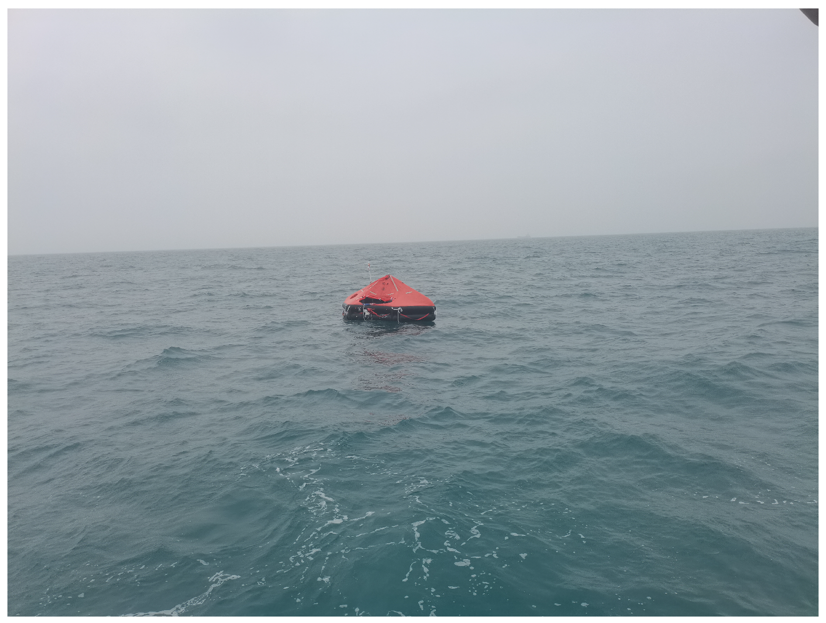
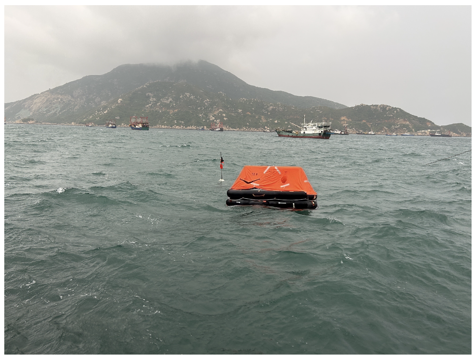
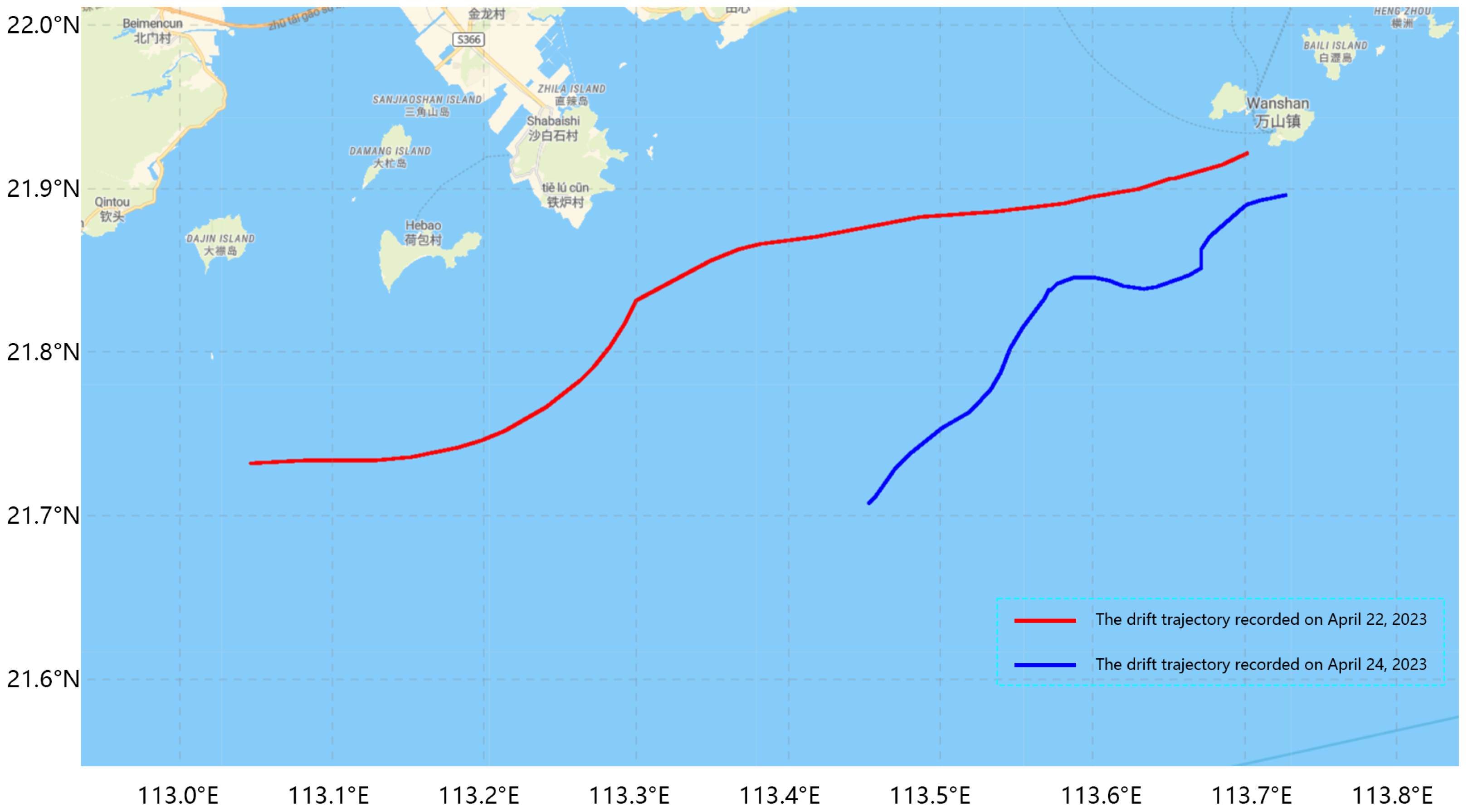
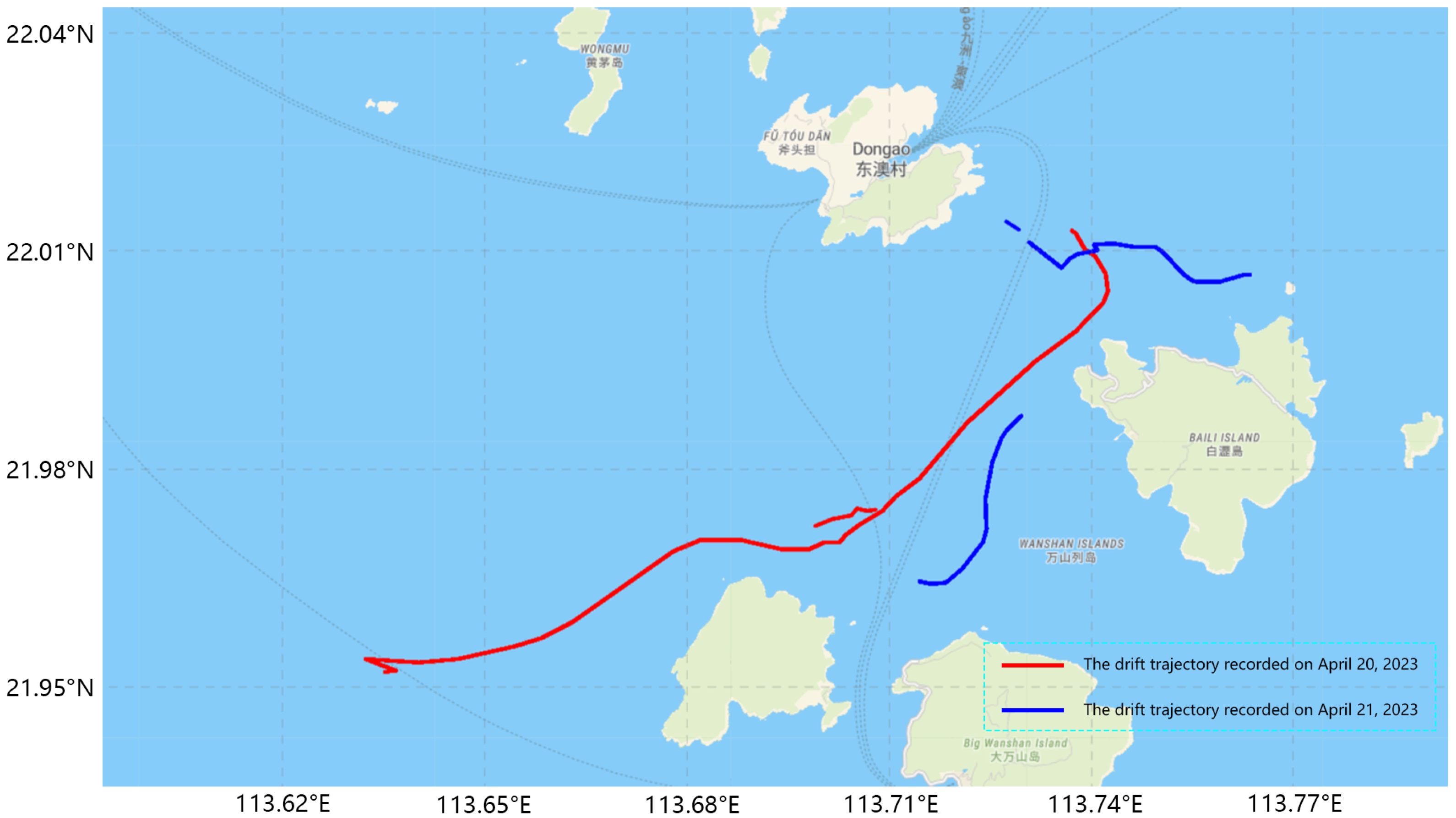
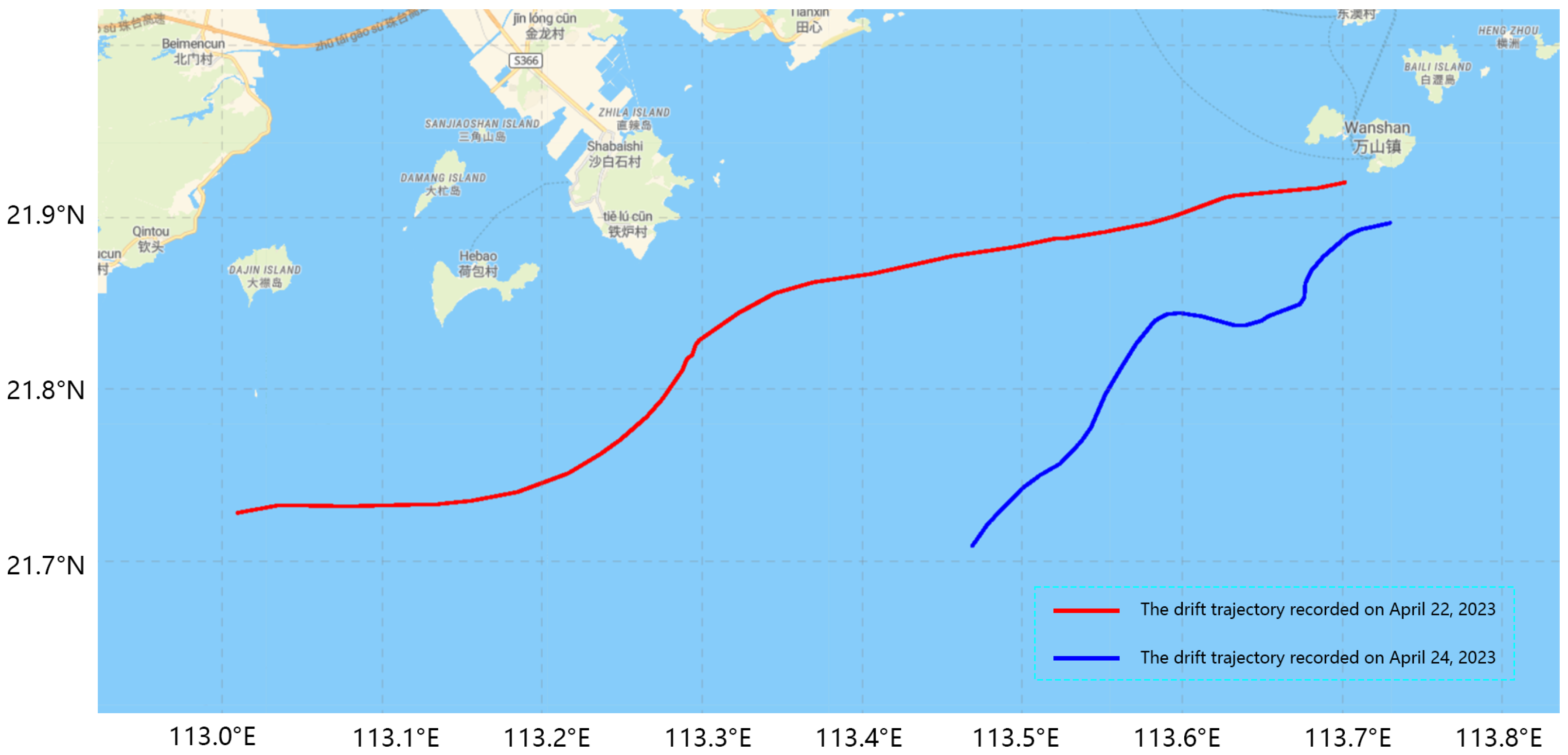
The observation experiments for the half-loaded life raft were conducted on four separate occasions, yielding a total of seven distinct drift trajectories. Specifically, two trajectories were recorded in open-sea areas (see Figure 11), while the remaining five were documented in island and reef regions (see Figure 12). The cumulative duration of the experiments was approximately 72 h, during which 566 data samples were collected in the open-sea areas and 222 samples in the island and reef areas.

The observation experiments for the fully loaded life raft were conducted twice, yielding two drift trajectories, as shown in Figure 13. The total duration of these experiments was approximately 48 h, during which a total of 566 drift samples were collected.

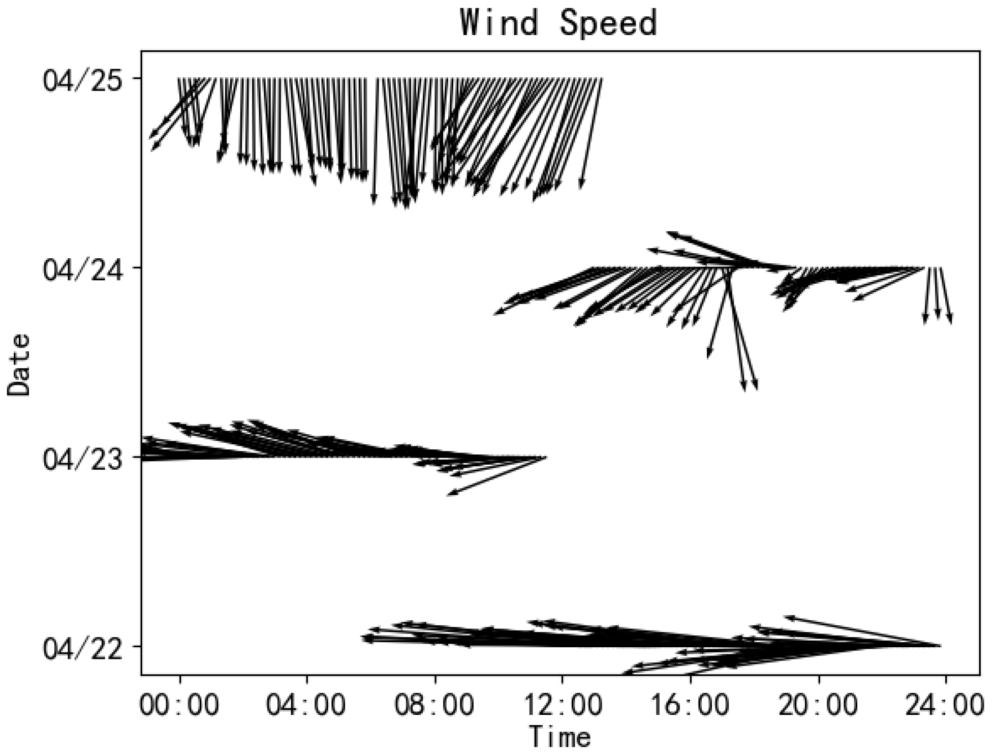
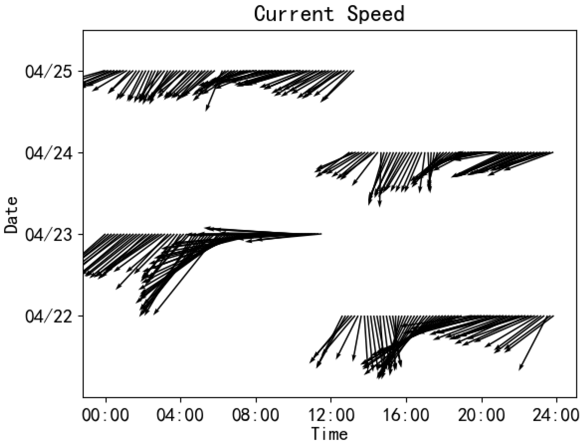
The 10 m wind speed in the open-sea experimental area fluctuates over time, as illustrated in Figure 14. Similarly, the current speed in the same area exhibits notable temporal variation, as illustrated in Figure 15.

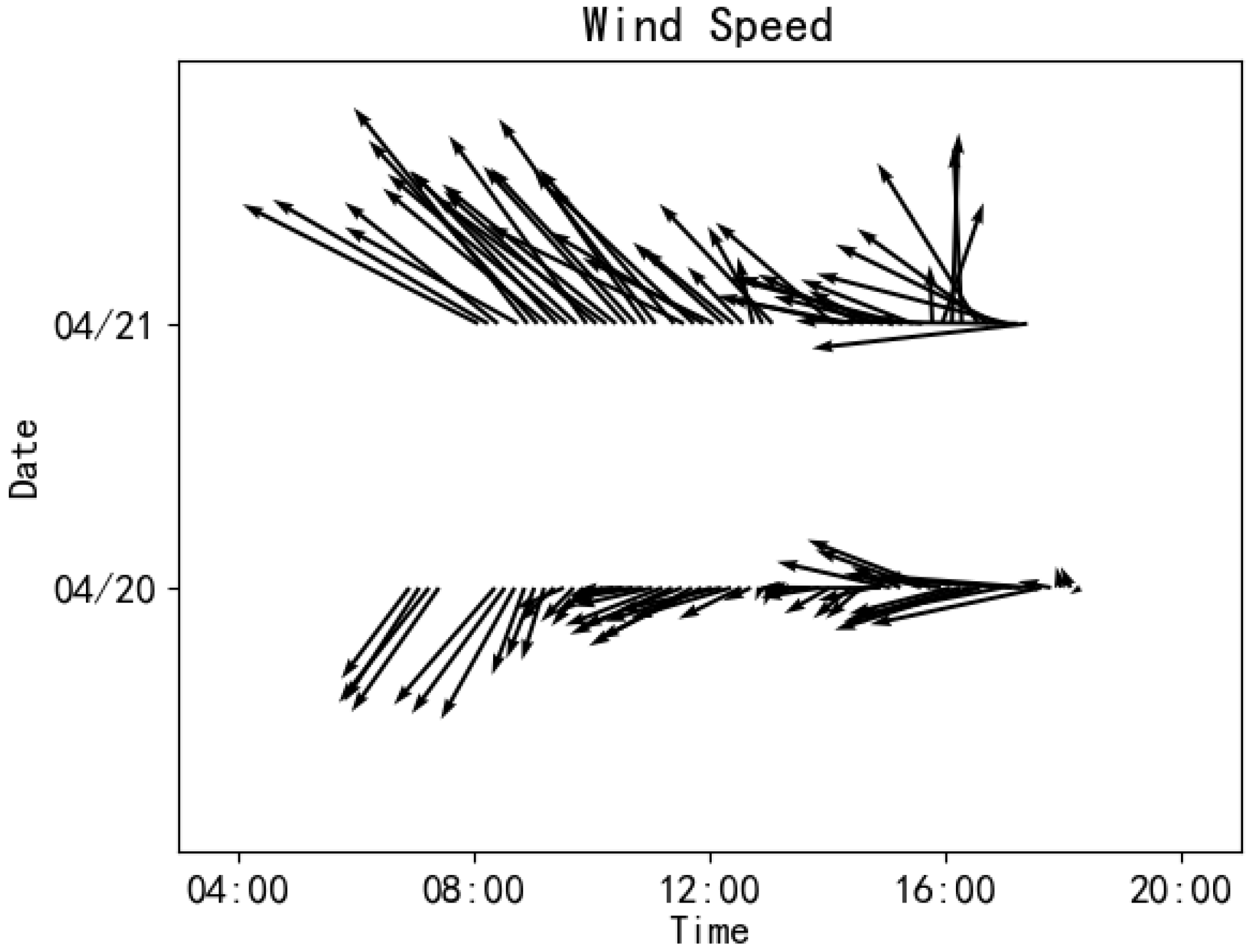
The 10 m wind speed in the island and reef experimental area exhibits temporal variability, as depicted in Figure 16. Similarly, the current velocity in the same region demonstrates similar fluctuations over time, as illustrated in Figure 17.

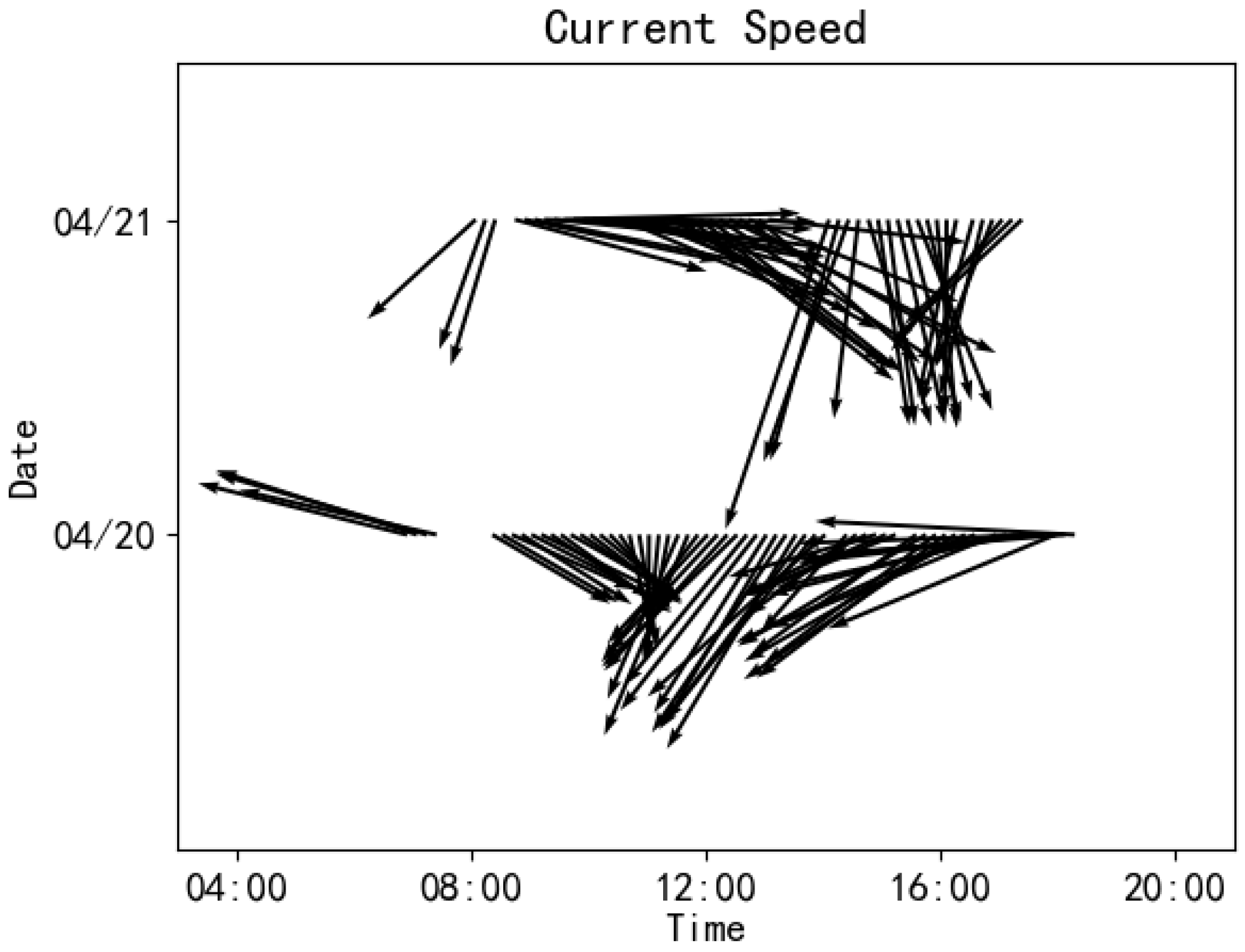
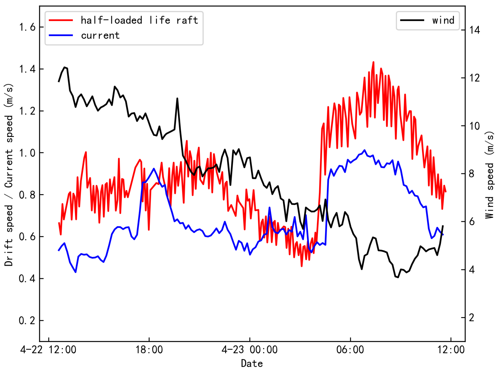
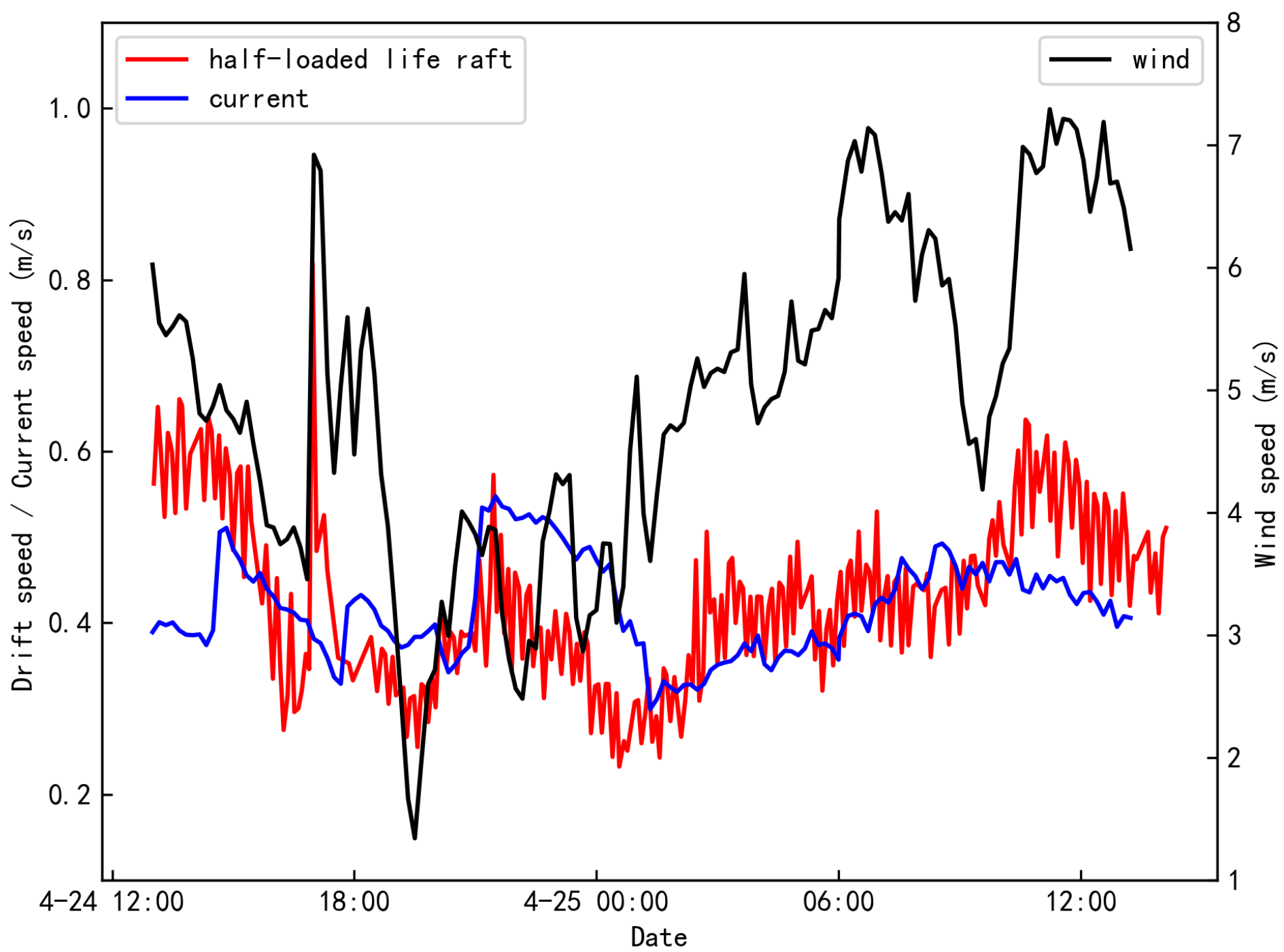
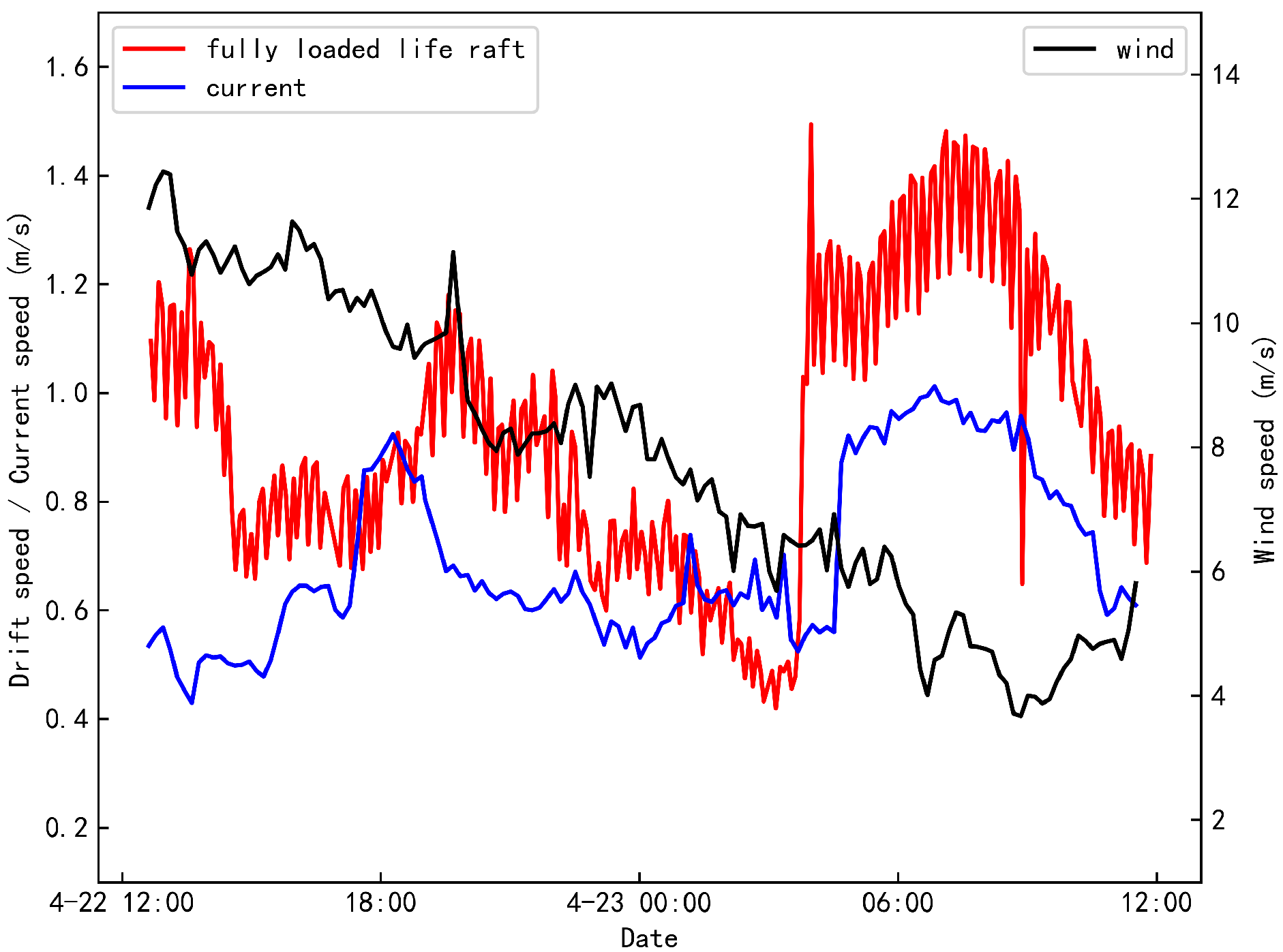
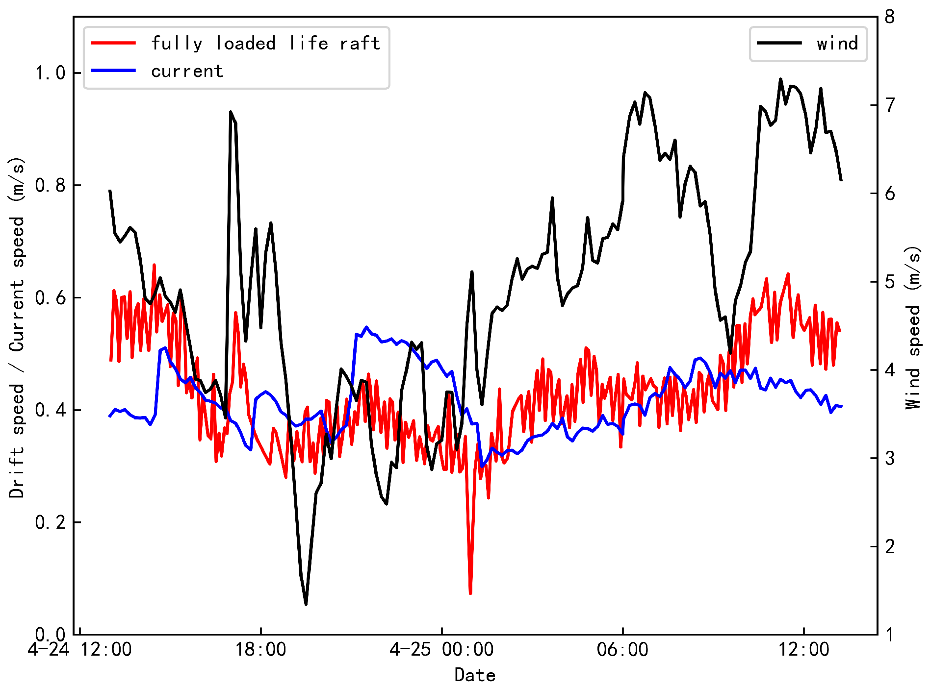
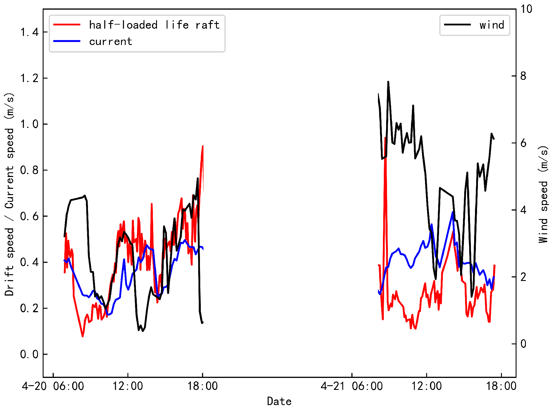
To facilitate a comprehensive visual comparative analysis of the relationships among wind speed, current speed, and the drift velocity of the experimental objects, time-series plots were constructed. In these plots, the x-axis represents time, the left y-axis denotes the scales for both target drift velocity and current speed, while the right y-axis indicates the scale for wind speed. The black line represents wind speed measured at 10 m above sea surface, the blue line indicates surface current speed, and the red line depicts the drift velocity of the experimental objects.

The variation curves of the target drift velocity, wind speed, and current speed for half-loaded life rafts under open-sea conditions are illustrated in Figure 18 and Figure 19. Similarly, Figure 20 and Figure 21 depict these variations for fully loaded life rafts. It is evident that the drift velocities of both configurations exhibit a strong correlation with the trends in current speed. Specifically, on April 23, an increase in current speed was accompanied by a corresponding rise in the drift velocity of the half-loaded life raft, indicating that in open-sea, the drift velocity of the half-loaded life raft is more significantly influenced by current speed than by wind speed. Furthermore, under identical current and wind conditions, the drift velocity of the fully loaded life raft shows greater sensitivity to changes in current speed.

The variation curves of target drift velocity, wind speed, and current speed for the half-loaded life raft within the islands and reefs region are depicted in Figure 22. The drift velocity of the half-loaded life raft exhibits a strong correlation with the trends in current speed. During the experiment conducted on April 20, the current speed initially decreased before increasing, and the drift velocity of the life raft followed this pattern closely. On April 21, the current speed peaked at 0.6 m/s while the wind speed remained relatively stable. Consequently, the drift velocity of the half-loaded life raft increased in accordance with the rise in current speed, demonstrating a consistent trend. These observations indicate that in island and reef sea areas, the drift velocity of the half-loaded life raft is predominantly influenced by current rather than wind.

The probability of wind-induced lateral drift deviation quantifies the likelihood that a floating object at sea will deviate from its original trajectory due to wind forces. Specifically, the probability of rightward deviation under lateral wind forcing is defined as the proportion of the +CWL samples relative to the total number of observations, whereas the probability of leftward deviation corresponds to the proportion of –CWL samples. This probability is influenced by multiple factors, including wind intensity, wind direction, the geometric configuration of the drifting object, and its mass distribution. Generally, stronger winds tend to increase the susceptibility of floating objects to lateral wind pressure, thereby enhancing the likelihood of course deviation.

After the removal of outliers, the total number of samples, as well as the counts of +CWL and –CWL samples obtained from the maritime drift target tracking experiments, are summarized in

Table 4. Statistical summary of crosswind occurrences and jibing frequency.

Object	Area	Sample Size	Number of +CWL Samples	Number of –CWL Samples	Jibing Frequency
Half-loaded life raft	Open sea	228	134 (58.7%)	94 (41.3%)	4.2%/h
	Islands and reefs	98	48 (49.0%)	50 (51.0%)	16.6%/h
Fully loaded life raft	Open sea	224	132 (58.9%)	92 (41.1%)	4.2%/h

. Based on the data in Table 4, the following observations can be made:

• Half-loaded life raft in open sea:
  The total number of samples is 228, of which 134 samples exhibited +CWL, accounting for 58.7%, while 94 samples exhibited –CWL, representing 41.3%. Consequently, the probability of rightward deviation due to lateral wind pressure for a half-loaded life raft is 58.7%. During approximately 48 h of open-sea observation, two jibing events were recorded, resulting in a calculated jibing frequency of 4.2%/h.
• Half-loaded life raft in the island and reef areas:
  The total number of samples is 98, of which 48 samples exhibited +CWL, constituting 49%, and 50 samples exhibited –CWL, accounting for 51%. Consequently, the probability of rightward deviation caused by lateral wind pressure for a half-loaded life raft is 49%. In this region, four jibing events were observed over a 24 h period, yielding a jibing frequency of 16.6%/h.
• Fully loaded life raft in open sea:
  The total number of samples is 224, of which 132 samples exhibited +CWL, representing 58.9%, while 92 samples exhibited –CWL, accounting for 41.1%. Consequently, the probability of rightward deviation caused by lateral wind pressure for a fully loaded life raft is 58.9%. Over a 48 h observation period, two jibing events were recorded, corresponding to a jibing frequency of 4.2%/h.

For both half-loaded and fully loaded life rafts, the probability of rightward deviation caused by lateral wind pressure is generally higher than that of leftward deviation. This indicates that under downwind conditions, the overall drift direction of these rafts tends to shift to the right. This rightward bias is likely the result of multiple factors, including geographical features that influence wind direction and speed, the effects of ocean currents, and the physical characteristics—such as shape and stability—of the drifting objects.

4.2. Establishment of AP98 Leeway Model

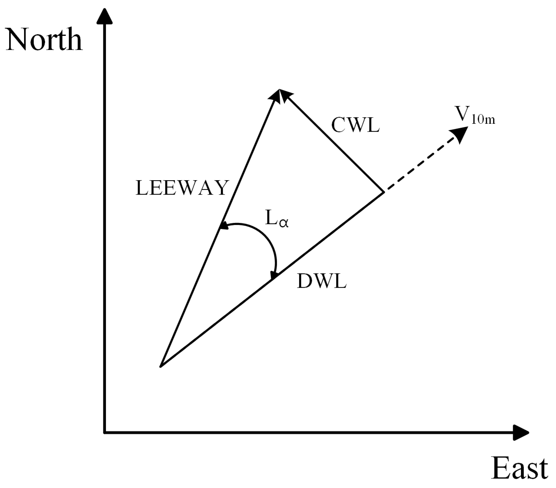
Given the complexity of the marine environment and the inherent hysteresis in the oceanic target response, this study processed experimental data at 10-min intervals by averaging the measurements over each interval. The wind-induced pressure velocity of the target was determined by subtracting the actual target’s drift velocity from the sea surface velocity. Thereafter, the wind-driven drift velocity was resolved into two orthogonal components: downwind (DWL) and crosswind (CWL). Finally, the linear correlation coefficient between the wind pressure velocity and the 10 m wind speed at the sea surface was calculated using the least squares method.

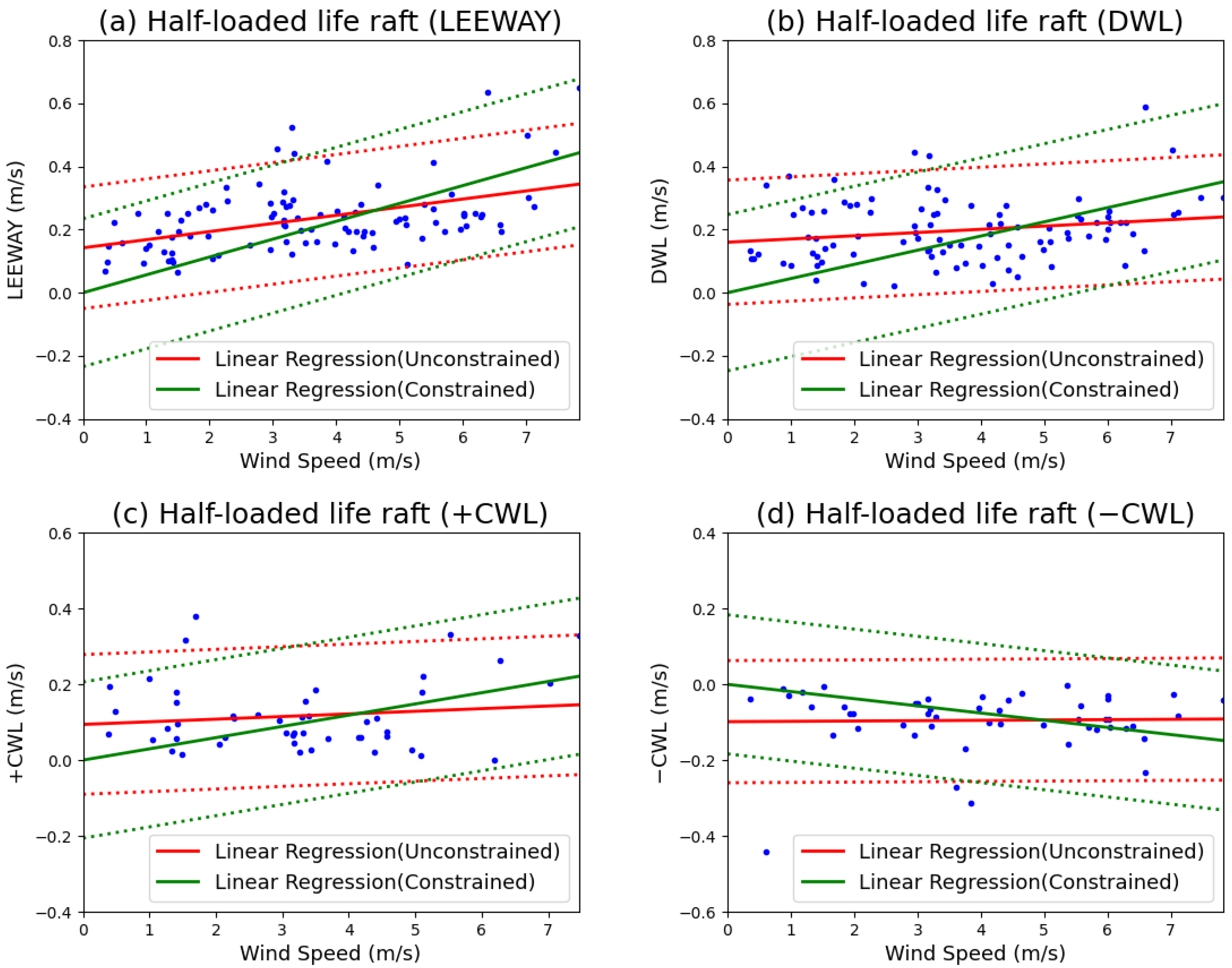
The linear regression results of the AP98 leeway model for the half-loaded life raft in open sea are illustrated in Figure 23, with the corresponding model parameter calibration results detailed in

Table 5. AP98 leeway model parameters for half-loaded life raft in open sea.

	Constrained Linear Regression		Unconstrained Linear Regression
	Slope (%)	Standard Deviation (cm/s)	Slope (%)	Intercept (cm/s)	Standard Deviation (cm/s)
Leeway	4.70	17.6	6.14	$-10.9$	17.3
DWL	4.04	17.3	5.83	$-13.6$	16.8
+CWL	2.05	9.60	2.20	$-1.22$	9.60
−CWL	$-1.79$	7.75	$-0.59$	$-6.98$	7.63

. These results demonstrate a strong linear relationship between both the downwind wind-induced drift velocity component (DWL) and the crosswind wind-induced drift velocity component (CWL) with reference to wind speed recorded at a height of 10 m over the sea surface.

From Figure 23, the following observations are made:

• The 10 m wind speed in the sample ranges from 2 to 13 m/s. The downwind component of wind-induced drift velocity ranges from −0.1 to 1 m/s. The slope obtained from unconstrained linear regression is 5.83%, with a standard deviation of 16.8 cm/s, whereas the slope obtained from constrained linear regression is 4.04%, accompanied by a standard deviation of 17.3 cm/s.
• The crosswind-induced drift velocity in the rightward direction ranges from −0.05 to 0.45 m/s. For unconstrained linear regression, the slope is 2.20%, with a standard deviation of 9.60 cm/s, whereas for constrained linear regression, the slope increases to 2.05%, with a standard deviation of 9.60 cm/s.
• The crosswind-induced drift velocity in the leftward direction ranges from −0.4 to 0.05 m/s. For unconstrained linear regression, the slope is −0.59%, with a standard deviation of 7.63 cm/s, while for constrained linear regression, the slope decreases to −1.79%, with a standard deviation of 7.75 cm/s.

In summary, superior calibration performance of the AP98 leeway model for a half-loaded life raft in open-sea conditions was achieved through the use of unconstrained linear regression. Consequently, based on the findings from the unconstrained linear regression analysis, the AP98 leeway model for the half-loaded life raft in offshore environments can be formulated as follows:

$$\left\{\begin{array}{c}\overrightarrow{L_d}=5.83\%W_{\mathrm{wind}}-13.6/100,\hfill \\ \overrightarrow{L_{c+}}=2.20\%W_{\mathrm{wind}}-1.22/100,\hfill \\ \overrightarrow{L_{c-}}=-0.59\%W_{\mathrm{wind}}-6.98/100.\hfill \end{array}\right.$$

(8)

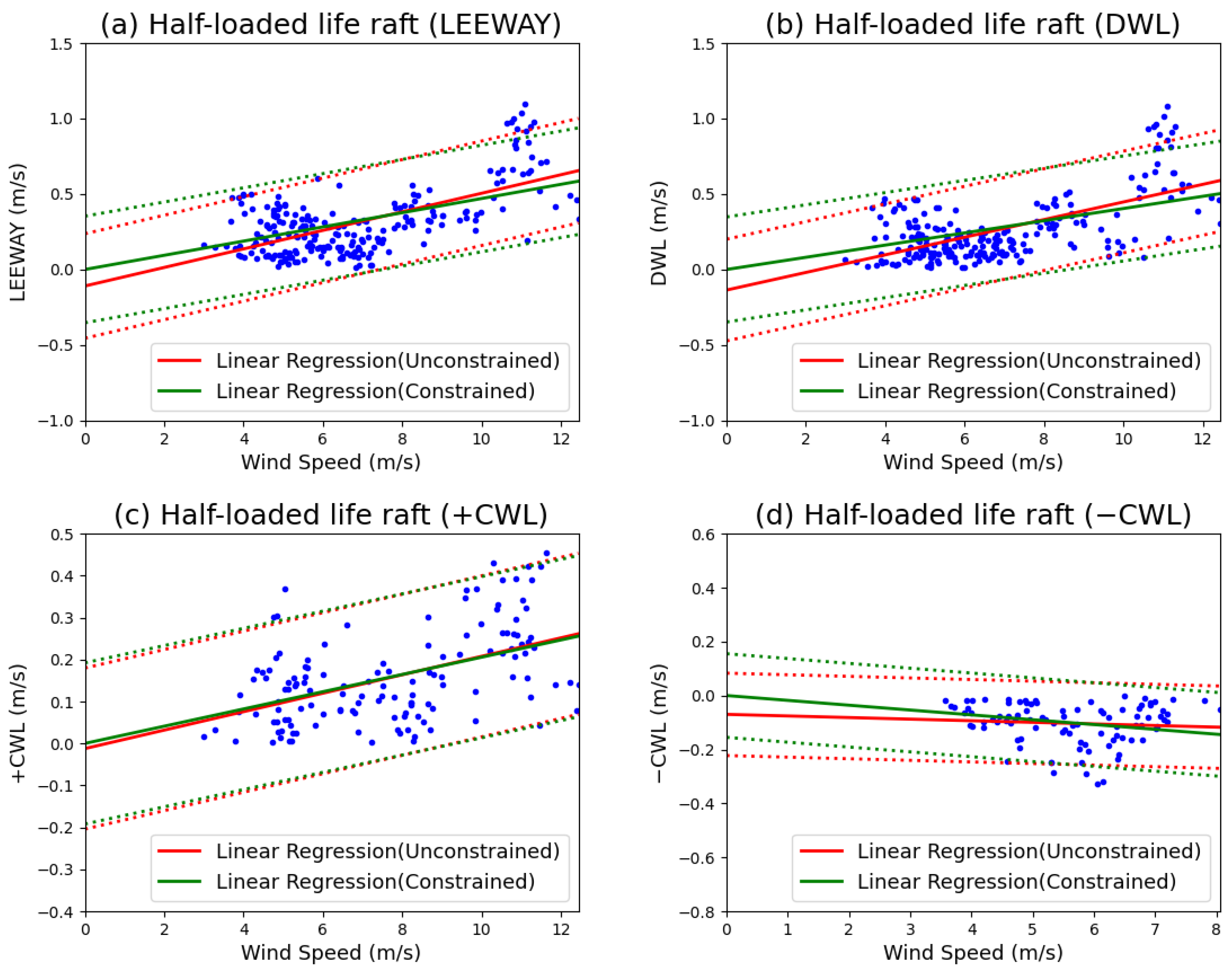
The linear regression analysis of the AP98 leeway model for the half-loaded life raft in the island and reef areas is presented in Figure 24. The corresponding model parameter calibration results are summarized in

Table 6. AP98 leeway model parameters for half-loaded life raft in island and reef areas.

	Constrained Linear Regression		Unconstrained Linear Regression
	Slope (%)	Standard Deviation (cm/s)	Slope (%)	Intercept (cm/s)	Standard Deviation (cm/s)
Leeway	5.65	11.71	2.57	14.22	9.62
DWL	4.49	12.3	1.02	15.9	9.83
+CWL	2.96	10.29	0.69	9.41	9.21
−CWL	$-1.89$	9.17	0.08	$-9.85$	8.06

. These findings indicate a robust linear relationship between both the downwind wind-induced drift velocity component (DWL) and the crosswind wind-induced drift velocity component (CWL) with the wind speed measured at 10 m above the sea surface.

From Figure 24, the following observations are made:

• The 10 m wind speed in the sample ranges from 0 m/s to 8 m/s. The downwind wind-induced drift velocity varies between 0 and 0.6 m/s. The slope obtained from unconstrained linear regression is 1.02%, with a standard deviation of 9.83 cm/s, whereas the slope obtained from constrained linear regression is 4.49%, accompanied by a standard deviation of 12.3 cm/s.
• The crosswind-induced drift velocity in the rightward direction ranges from 0 m/s to 0.4 m/s. For unconstrained linear regression, the slope is 0.69%, with a standard deviation of 9.21 cm/s, whereas for constrained linear regression, the slope increases to 2.96%, with a standard deviation of 20.29 cm/s.
• The crosswind-induced drift velocity in the leftward direction ranges from −0.43 m/s to 0 m/s. For unconstrained linear regression, the slope is 0.08%, with a standard deviation of 8.06 cm/s, while for constrained linear regression, the slope decreases to −1.89%, with a standard deviation of 9.17 cm/s.

In summary, superior calibration performance of the AP98 leeway model for a half-loaded life raft in island and reef waters was achieved through the use of unconstrained linear regression. Therefore, based on these findings, the AP98 leeway model for the half-loaded life raft in the island and reef areas can be expressed as follows:

$$\left\{\begin{array}{c}\overrightarrow{L_d}=1.02\%W_{\mathrm{wind}}+15.9/100,\hfill \\ \overrightarrow{L_{c+}}=0.69\%W_{\mathrm{wind}}+9.41/100,\hfill \\ \overrightarrow{L_{c-}}=0.08\%W_{\mathrm{wind}}-9.85/100.\hfill \end{array}\right.$$

(9)

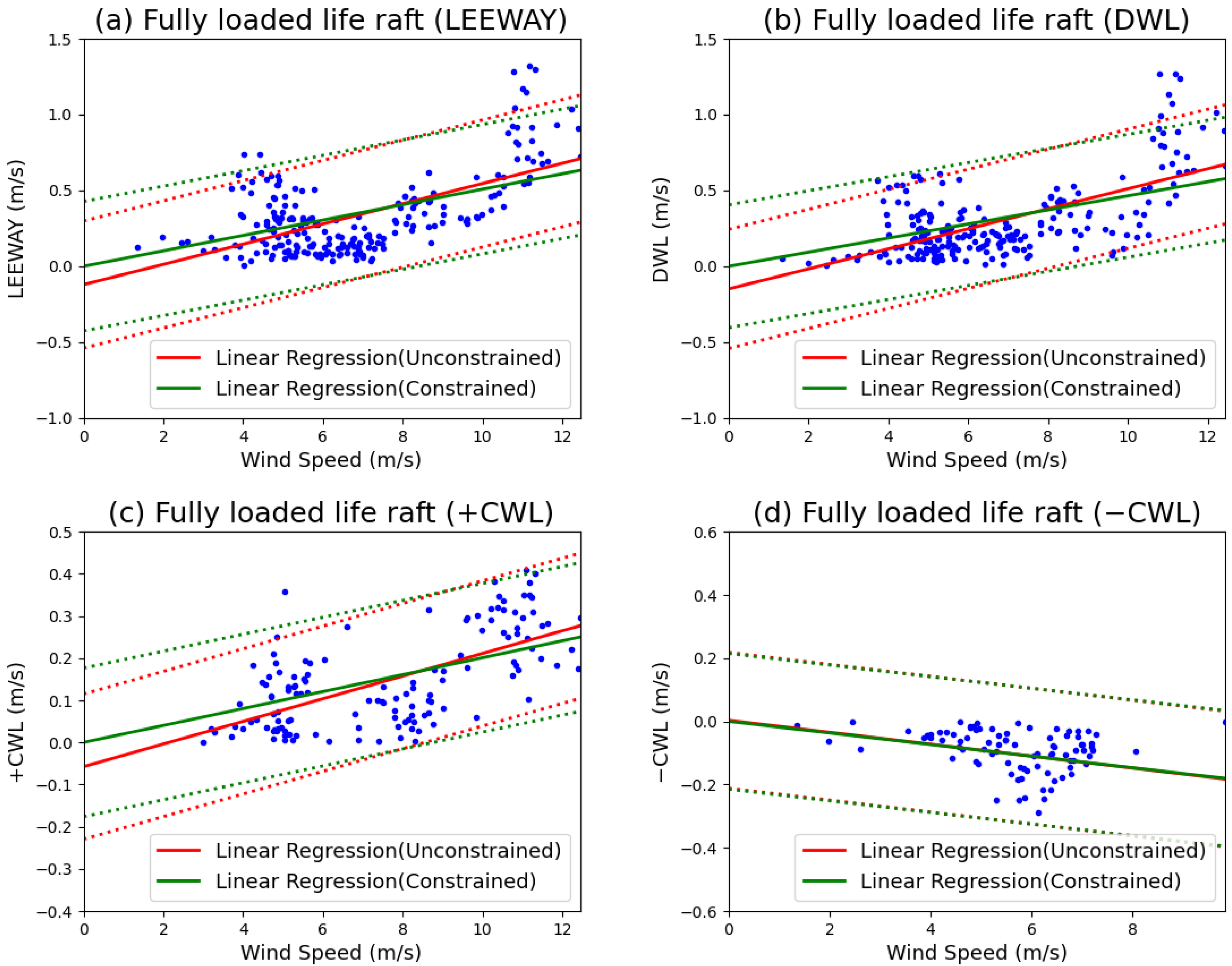
The linear regression analysis of the AP98 leeway model for fully loaded life rafts in open sea is presented in Figure 25. Detailed calibration results for the model parameters are provided in Table 7. The analysis reveals a significant linear relationship between the downwind wind-induced drift velocity component (DWL) and the crosswind wind-induced drift velocity component (CWL), both correlated with the wind speed at 10 m above sea level. Key observations from this analysis include the following:

• The 10 m wind speed in the sample ranges from 1.0 m/s to 12.5 m/s, whereas the downwind wind-induced drift velocity varies between −0.2 m/s and 1.3 m/s. The slope obtained from unconstrained linear regression is 6.60%, with a standard deviation of 19.63 cm/s. By comparison, the slope derived from constrained linear regression is 4.64%, accompanied by a slightly higher standard deviation of 20.24 cm/s.
• The crosswind-induced drift velocity in the rightward direction ranges from −0.05 m/s to 0.35 m/s. The slope derived from unconstrained linear regression is 2.68%, with a standard deviation of 8.61 cm/s, whereas the slope obtained from constrained linear regression is 2.01%, accompanied by a standard deviation of 8.81 cm/s.
• The crosswind-induced drift velocity in the leftward direction ranges from −0.4 m/s to 0 m/s. An unconstrained linear regression yields a slope of −1.88% with a standard deviation of 10.73 cm/s, while the constrained regression produces a similar slope of −1.83%, with the same standard deviation.

Table 7. AP98 leeway model parameters for fully loaded life raft in open sea.

	Constrained Linear Regression		Unconstrained Linear Regression
	Slope (%)	Standard Deviation (cm/s)	Slope (%)	Intercept (cm/s)	Standard Deviation (cm/s)
Leeway	5.08	21.3	6.66	$-12.1$	20.9
DWL	4.64	20.2	6.60	$-14.9$	19.6
+CWL	2.01	8.81	2.68	$-5.75$	8.61
−CWL	$-1.83$	10.7	$-1.88$	0.31	10.7

Table 7. AP98 leeway model parameters for fully loaded life raft in open sea.

	Constrained Linear Regression		Unconstrained Linear Regression
	Slope (%)	Standard Deviation (cm/s)	Slope (%)	Intercept (cm/s)	Standard Deviation (cm/s)
Leeway	5.08	21.3	6.66	$-12.1$	20.9
DWL	4.64	20.2	6.60	$-14.9$	19.6
+CWL	2.01	8.81	2.68	$-5.75$	8.61
−CWL	$-1.83$	10.7	$-1.88$	0.31	10.7

Figure 25. Linear regression results for fully loaded life raft in open sea. The dotted lines indicate the ±2 standard error bounds of the fitted regression lines.

Figure 25. Linear regression results for fully loaded life raft in open sea. The dotted lines indicate the ±2 standard error bounds of the fitted regression lines.

In summary, superior calibration performance of the AP98 leeway model for a fully loaded life raft in open-sea conditions was achieved through the use of unconstrained linear regression. Consequently, based on the findings from the unconstrained linear regression analysis, the AP98 leeway model for a fully loaded life raft in open-sea conditions can be formulated as follows:

$$\left\{\begin{array}{c}\overrightarrow{L_d}=6.60\%W_{\mathrm{wind}}-14.92/100,\hfill \\ \overrightarrow{L_{c+}}=2.68\%W_{\mathrm{wind}}-5.75/100,\hfill \\ \overrightarrow{L_{c-}}=-1.88\%W_{\mathrm{wind}}+0.31/100.\hfill \end{array}\right.$$

(10)

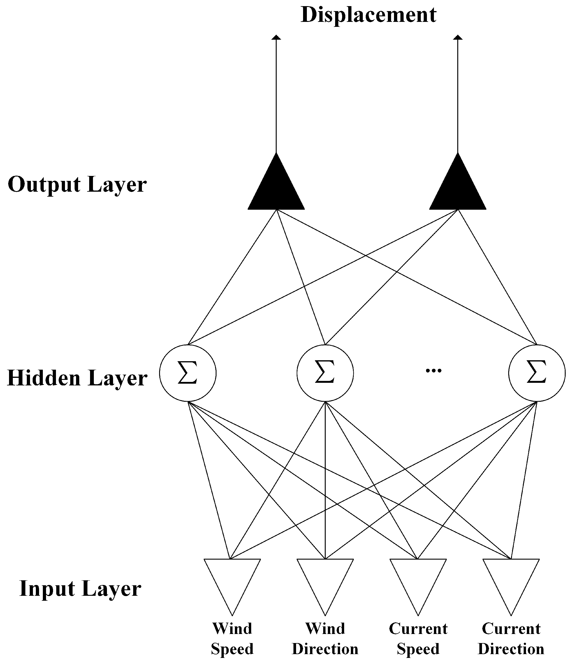
4.3. Establishment of BP Neural Network Model

This section focuses on developing a drift trajectory prediction model for maritime distress targets using a BP neural network and on performing a comparative evaluation of different target-specific models based on defined performance metrics. A comprehensive dataset consisting of 2346 data samples was compiled through maritime tracking and drift observation experiments. The dataset was initially classified according to target type and subsequently divided into training and testing subsets in a 3:1 ratio. The training set was used to fit the neural network model, while the testing set, reserved as the final validation set, was excluded from the training process to ensure an unbiased evaluation of the prediction model.

Following data filtering, analysis, and dataset partitioning, the prepared datasets were employed to train the BP neural network, yielding drift trajectory prediction models specifically tailored to various target types and maritime regions. The training process encompasses forward propagation, wherein input data pass through the network layers, undergoing transformations via weights and activation functions to produce the final outputs. The model’s output is compared with actual results to compute the prediction error, which is then propagated backward to adjust the network’s weights and minimize the error. This process employs the gradient descent optimization algorithm to determine each weight’s contribution to the error and iteratively update the weights. Training of the BP neural network involves repeated cycles of forward and backward propagation.

The objective of the training is to minimize the error between predicted outputs and actual labels, ensuring the model can effectively fit the training data and generalize well to unseen data. Several factors are critical to the training performance of the BP neural network, including the following:

• Selecting an appropriate loss function to quantify prediction error;
• Determining the network architecture and hyperparameters;
• Initializing weights appropriately to prevent suboptimal convergence;
• Choosing suitable activation functions to facilitate nonlinear transformations;
• Setting an optimal learning rate to balance the speed and stability of convergence.

During the model training process, the effectiveness of training is evaluated by monitoring the decreasing trend of error values output by the neural network in each iteration. To prevent overfitting, three-fold cross-validation is utilized. Furthermore, learning curves are employed to visualize the training performance, enabling an intuitive assessment of the training state through analysis of the plotted curves.

Optimal parameters for each model were identified through systematic manual hyperparameter tuning, considering the characteristics of the dataset and comparative analyses of model performance across various parameter configurations. The selected optimal parameters are summarized in

Table 8. Optimal parameters of models for drift targets in different sea areas.

Object	Area	Number of Neurons	Learning Rate	Number of Generations	RMSE
Half-loaded Life Raft	Open sea	1000	0.05	25,000	0.3
	Islands and reefs	1000	0.05	20,000	0.2
Fully loaded Life Raft	Open sea	900	0.04	25,000	0.36

.

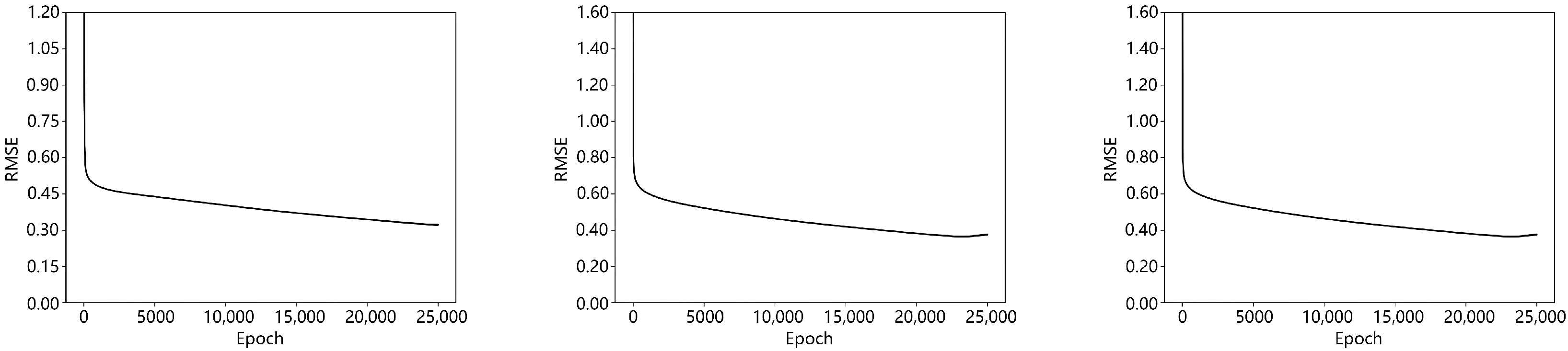
As shown in Figure 26, the training errors of the BP neural network models exhibit a consistent decreasing trend with an increasing number of training iterations across all three life raft drift scenarios. For the half-loaded life raft in open sea (left curve), the training error gradually decreases and stabilizes after approximately 25,000 iterations, with the root mean square error (RMSE) converging to around 0.3. In the island and reef scenario with a half-loaded raft (center curve), convergence is achieved slightly earlier, around 20,000 iterations, with a lower final RMSE of approximately 0.2. For the fully loaded raft in open sea (right curve), the model also demonstrates steady error reduction, plateauing at around 25,000 iterations, with a final RMSE of approximately 0.36. These results indicate effective convergence behavior under varying loading conditions and environmental contexts, with differences in RMSE reflecting the impact of drift complexity on prediction accuracy.

5. Comparison and Discussion

The establishment of drift trajectory prediction models utilizing the AP98 leeway model and the BP neural network model offers a solid technical foundation for forecasting the trajectories of maritime drifting objects. By employing these two models, this study enables the simulation of a target’s drift trajectory over a specified period through the input of initial position, wind data, current data, and the application of the Lagrangian particle tracking method.

The normalized cumulative Lagrangian value (s) is introduced as a metric to quantitatively and intuitively assess the performance of prediction models. This metric offers a precise measure of the discrepancy between predicted and actual trajectories. The formula for calculating it is given by

$$s=\sum _{i=1}^N{d}_i/\sum _{i=1}^N{l}_{oi}$$

(11)

where $d_i$ denotes the distance between the predicted and actual positions in the Lagrangian trajectory over a unit time interval, $l_{oi}$ represents the length of the corresponding segment of the actual trajectory, and N is the total number of such intervals. A smaller s-value indicates superior model performance. The s-value statistics comparing the predicted trajectories from the AP98 leeway model and the BP neural network model against the actual trajectories for various target types are summarized in

Table 9. Statistical results of s values for predicted and actual trajectories for AP98 leeway model and BP neural network model.

Object	Area	s Value for AP98 Model	s Value for BP Neural Network Model
Half-loaded life raft	Open sea	0.67	1.29
	Islands and reefs	0.29	0.35
Fully loaded life raft	Open sea	0.66	0.79

. As shown in Table 9, in open-sea conditions, the AP98 leeway model exhibits marginally better performance than the BP neural network model in predicting the drift trajectory of the half-loaded life raft. In island and reef areas, the prediction performance of both models is comparable, indicating similar levels of accuracy.

In practical scenarios, the irregular geometric structure of drifting targets leads to forces that diverge from theoretical predictions. Moreover, measurement inaccuracies and the impact of numerous random factors significantly complicate the accurate computation of drift trajectories. However, the Monte Carlo method offers an effective approach for simulating the search and rescue area of maritime distressed targets, thereby enhancing the precision of prediction outcomes. Using this method, 1000 particles are initialized at the target’s initial position. Each particle undergoes drift motion influenced by stochastic perturbations, ultimately resulting in a distribution of the final positions of these 1000 simulated particles. To incorporate the effect of crosswind-induced drift deviation (CWL), each particle is initially assigned a deflection direction—either +CWL (rightward) or –CWL (leftward)—based on the relative counts of +CWL and –CWL samples obtained from the maritime drift target tracking experiments. This probabilistic assignment reflects the empirically observed likelihood of crosswind-induced drift direction, ensuring that the simulation accounts for initial directional bias in a realistic manner. Our implementation introduces a simple jibing mechanism: each particle has a small probability of switching CWL sign at each time step. For example, particles initialized with rightward drift may change to leftward and vice versa, depending on probabilistic thresholds derived from observed behavior. This mechanism allows the simulated trajectories to reflect more realistic directional oscillations during drift, partially capturing the effect of jibing observed in real-world conditions. As a result, the simulation not only accounts for initial drift bias but also accommodates dynamic shifts in drift direction, thereby improving the fidelity of search area prediction.

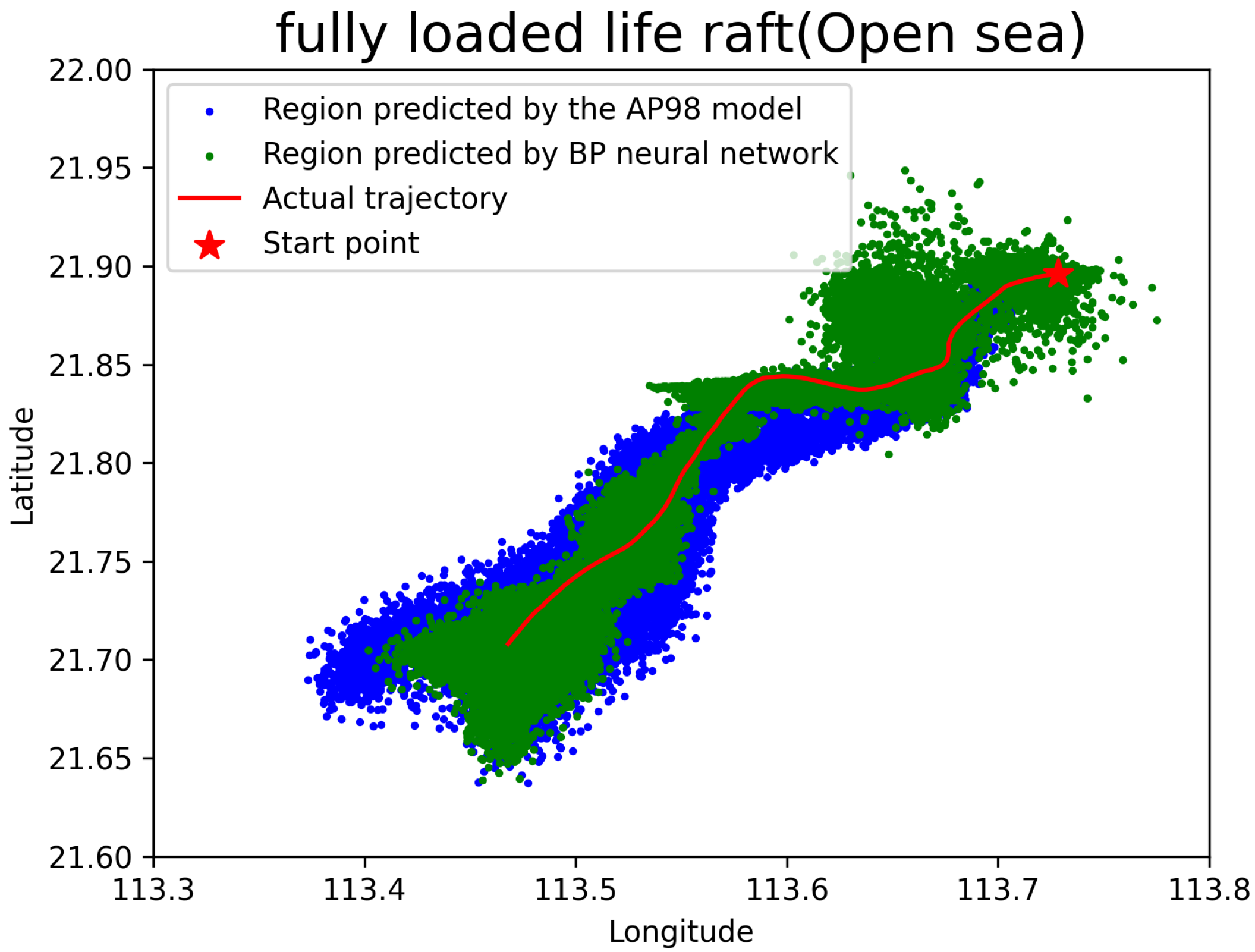
The POPC for a fully loaded life raft in the open sea, based on experimental observation data, is 58.9%. Therefore, out of 1000 simulated particles, 589 are subject to wind drift with a rightward bias, while the remaining 411 are subject to wind drift with a leftward bias. The Monte Carlo simulation results for the drift region of the fully loaded life raft in the open sea, using the AP98 leeway model, are illustrated in Figure 27.

Table 10. Average hourly deviation between predicted and actual drift positions of the fully loaded life raft in open sea (km).

Model	1H	2H	3H	4H	5H	6H	7H	8H	9H	10H	11H	12H	13H	14H	15H	16H	17H	18H	19H	Average Value
AP98	0.46	1.00	0.94	0.80	1.46	1.19	1.23	1.70	2.28	2.72	3.47	3.70	3.74	3.13	2.42	2.00	1.89	2.39	3.30	2.10
BP	1.99	3.41	2.88	1.42	2.08	1.53	1.42	1.55	1.23	1.25	1.57	1.92	2.32	2.96	1.78	2.08	1.97	2.12	1.78	1.96

presents the statistical summary of the mean distance errors calculated at each full-hour time point. At each hour, the Euclidean distances between the actual position and all 1000 simulated particle positions are computed, and the average of these distances is taken as the prediction error for that hour. The final error is obtained by averaging these hourly errors over the entire simulation period. From the figure, it is evident that the predicted results generally encompass the actual drift trajectory. Additionally, due to wind-induced crosswind drift, the prediction results based on the AP98 leeway model exhibit greater dispersion compared to the more concentrated predictions from the BP neural network model.

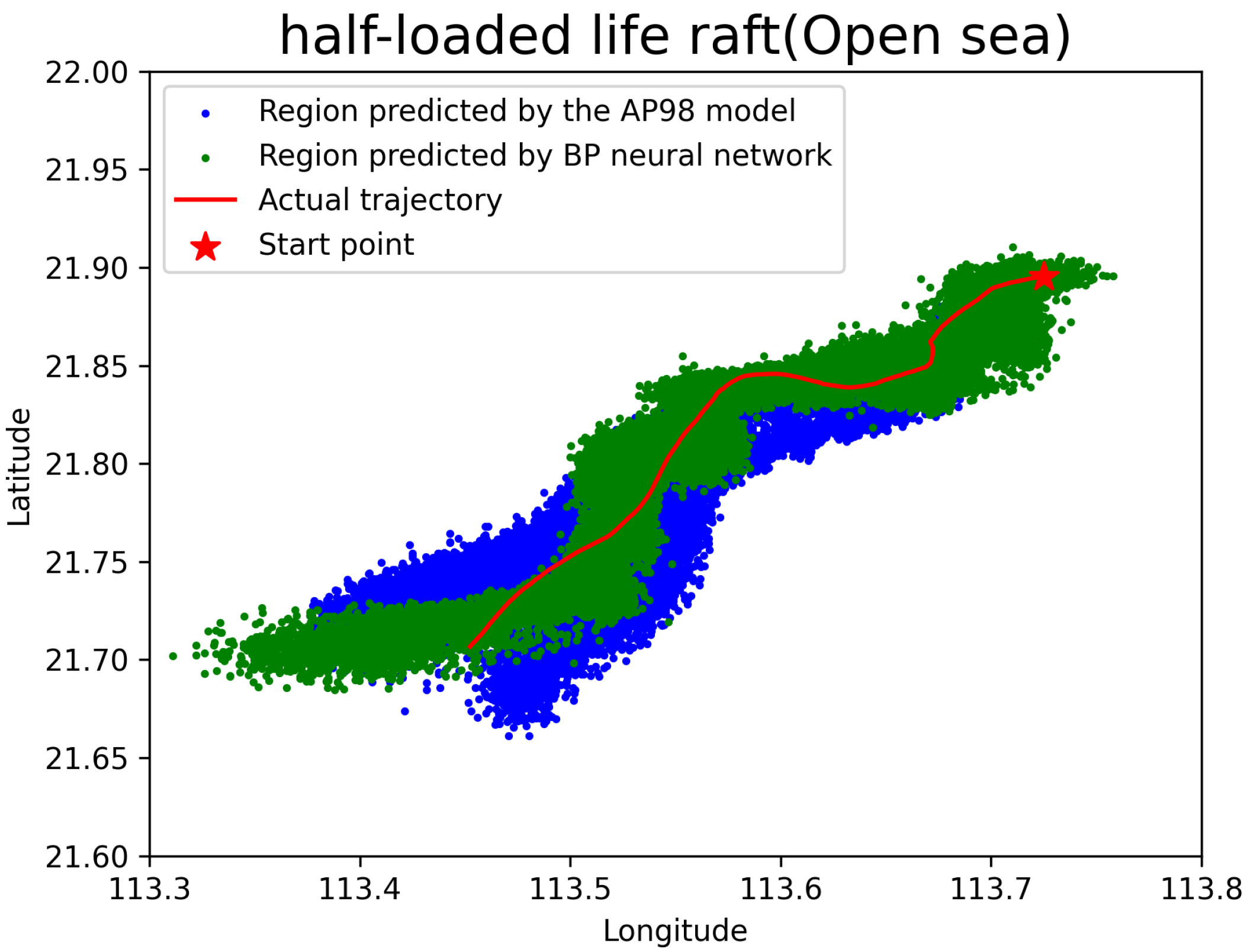
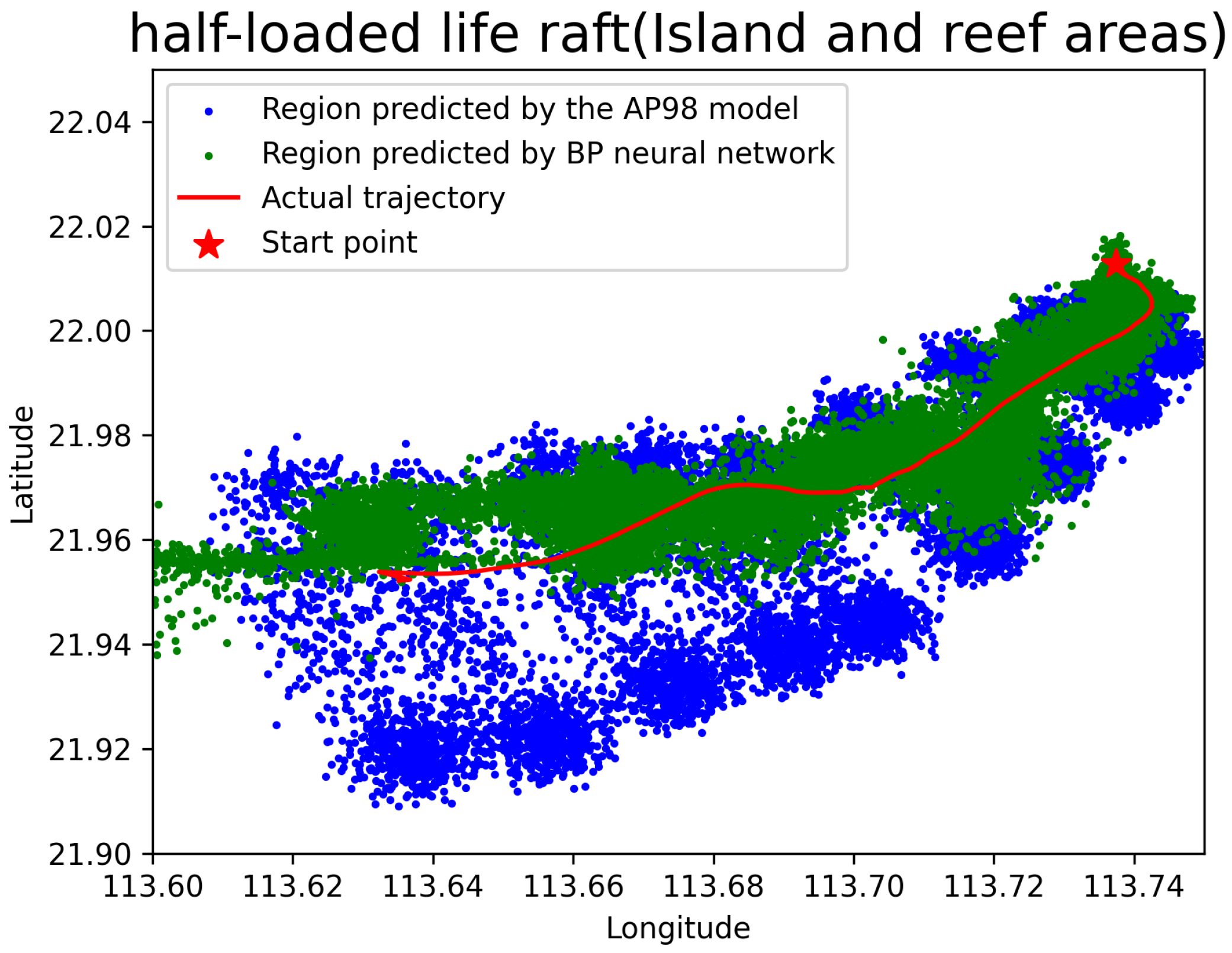
This method effectively integrates uncertainties and stochastic elements into the simulation, providing a more comprehensive and realistic prediction of potential drift areas. Such probabilistic modeling plays a critical role in improving the effectiveness of search and rescue operations by enabling broader coverage and increasing the likelihood of successful target localization. For a half-loaded life raft, the Probability of Crosswind Pressure Coefficient (POPC) derived from experimental observation data is 58.7% in offshore areas around islands and reefs and 49% in internal waters. Consequently, in open seas, 587 out of 1000 simulated particles are influenced by rightward crosswind-induced drift, while the remaining 413 particles are influenced by leftward crosswind-induced drift. In contrast, in island and reef areas, 490 out of 1,000 simulated particles experience rightward crosswind-induced drift, while the remaining 510 particles experience leftward crosswind-induced drift.

The Monte Carlo prediction results for the drift regions of the half-loaded life raft in two different sea areas, based on the AP98 leeway model and the BP neural network model, are presented in Figure 28 and Figure 29, respectively.

Table 11. Average hourly deviation between predicted and actual drift positions of the half-loaded life raft in open sea (km).

Model	1H	2H	3H	4H	5H	6H	7H	8H	9H	10H	11H	12H	13H	14H	15H	16H	17H	18H	19H	20H	21H	Average Value
AP98	0.87	1.40	1.44	2.04	2.19	2.02	2.10	2.30	2.51	2.88	3.08	2.96	2.51	2.02	1.92	2.07	2.40	2.93	3.70	4.14	4.78	2.49
BP	1.44	1.78	3.32	1.59	2.47	2.26	3.22	5.15	3.48	2.44	1.76	1.64	1.47	1.82	2.02	2.01	1.53	1.42	2.50	2.29	1.83	2.26

and

Table 12. Average hourly deviation between predicted and actual drift positions of the half-loaded life raft in island and reef waters (km).

Model	1H	2H	3H	4H	5H	6H	7H	8H	Average Value
AP98	0.49	0.67	1.43	1.71	1.88	2.17	2.50	2.56	1.68
BP	0.34	0.78	1.52	1.84	1.66	1.33	1.82	2.12	1.43

provide statistical summaries of the mean distance errors computed at each full-hour time point. For each hour, the Euclidean distances between the observed position and the 1000 simulated particle positions are calculated, and the mean of these distances represents the prediction error for that hour. The final reported value is the average of these hourly errors over the full simulation period. From the figures, it is evident that both models’ predicted drift regions encompass the actual drift trajectories. However, due to crosswind-induced lateral drift, the AP98 leeway model predicts a more dispersed drift region, reflecting a wider range of possible trajectories. In contrast, the BP neural network model predicts a more concentrated drift region, indicating a narrower and more focused set of probable drift paths.

6. Conclusions

This study presents an investigation into the drift prediction of life rafts in island and reef waters, based on field experiments conducted in the South China Sea. The drift characteristics of life rafts under varying load conditions were analyzed. Two predictive models–the AP98 leeway model and a BP neural network model–were developed and rigorously validated, with their predictive accuracies evaluated in both open-sea and island-reef environments. The experimental results indicate that the BP neural network model consistently demonstrates superior predictive performance compared to the AP98 leeway model across various maritime environments. While the AP98 model can offer reasonable predictions in open-sea conditions, its accuracy is notably inferior to that of the BP model. Particularly in complex island and reef regions—characterized by intricate hydrodynamics, narrow passages, and localized circulations—the BP model shows markedly enhanced accuracy and reduced deviation. In addition, the integration of Monte Carlo simulations into both models enhanced the robustness of the drift predictions. By incorporating stochastic perturbations into wind-induced drift coefficients and predicted displacements, the simulations effectively accounted for uncertainties inherent in both environmental conditions and model parameters. The results further demonstrate that the BP neural network model not only yields more concentrated and spatially accurate drift predictions but also exhibits lower average hourly deviation compared to the AP98 model in nearly all test cases. Overall, the BP neural network model demonstrates greater predictive accuracy than the AP98 leeway model for both half-loaded and fully loaded life rafts, regardless of maritime environment.

The experimental findings also reveal that fully loaded life rafts exhibit a greater rate of increase in drift velocity relative to current speed compared to half-loaded life rafts. This behavior is primarily attributed to the larger contact area with the water surface of fully loaded rafts, which enhances their responsiveness to current forces. Additionally, the divergence angle of wind-induced drift in the crosswind direction is greater in open-sea areas than in island and reef regions. However, the frequency of crosswind-induced turning events is lower in open-sea environments than in more complex island and reef waters. Moreover, the probability of rightward crosswind-induced turning is higher in open-sea regions, whereas leftward turning events are more frequently observed in island and reef areas. Furthermore, the drift velocities of life rafts in island and reef waters are generally lower than those observed in open-sea areas, likely due to the complex interactions between tidal currents, topography, and localized circulation patterns in these environments.

Although the present study is geographically centered on island and reef systems in the South China Sea, the employed methodology—grounded in the AP98 leeway model and validated through field observations—offers a transferable framework for drift prediction in analogous maritime settings. Nevertheless, the leeway response of drifting objects is known to be sensitive to regional wind patterns, sea states, and topographic features. As such, the direct application of the derived parameters to other geographic domains should be approached with caution. Regional recalibration based on local observational data is recommended to ensure the model’s fidelity in alternate environmental contexts.

It is important to note that the dataset employed in this study was obtained from a short-term (15-day) field experiment that covered both open-sea and island-reef regions in the South China Sea. While the spatial coverage includes different marine environments, the limited temporal scale of the data means that long-term effects such as global warming and climate change are unlikely to be reflected in the observations. As such, these factors were not explicitly incorporated into the current modeling framework. Nonetheless, we acknowledge that for long-term or climatologically oriented drift prediction studies, particularly those involving seasonal or interannual variability, it would be valuable to consider climate-induced changes in wind and current patterns. Future research could explore the integration of climate projections or multi-year observational datasets to enhance the model’s applicability under changing environmental conditions.