Design of Virtual Sensors for a Pyramidal Weathervaning Floating Wind Turbine

Abstract

This study explores virtual sensing techniques for the Eolink floating offshore wind turbine (FOWT), which features a pyramidal platform and a single-point mooring system that enables weathervaning to maximize power production and reduce structural loads. To address the challenges and costs associated with monitoring submerged components, virtual sensors are investigated as an alternative to physical instrumentation. The main objective is to design a virtual sensor of mooring hawser loads using a reduced set of input features from GPS, anemometer, and inertial measurement unit (IMU) data. A virtual sensor is also proposed to estimate the bending moment at the joint of the pyramid masts. The FOWT is modeled in OrcaFlex, and a range of load cases is simulated for training and testing. Under defined sensor sampling conditions, both supervised and physics-informed machine learning algorithms are evaluated. The models are tested under aligned and misaligned environmental conditions, as well as across operating regimes below- and above-rated conditions. Results show that mooring tensions can be estimated with high accuracy, while bending moment predictions also perform well, though with lower precision. These findings support the use of virtual sensing to reduce instrumentation requirements in critical areas of the floating wind platform.

1. Introduction

Floating offshore wind turbines (FOWTs) have undergone significant evolution in recent years, with various concepts being applied in industrial settings. To date, commercial floating wind farms include Equinor’s Hywind Tampen and Hywind Scotland, Principle Power’s Kincardine off the Scottish coast, and Ocean Winds’ WindFloat Atlantic off the coast of Portugal [1,2]. During the early stages of floating wind development, cost reduction has been identified as a key requirement for large-scale deployment. Remote monitoring remains a cost challenge in floating wind structures [3,4]. Reducing physical sensors in complex areas lowers procurement and maintenance needs, and virtual sensors offer a viable alternative [3,5].

This article is based on Eolink’s disruptive floating offshore wind turbine (FOWT) concept [6], which is primarily characterized by a single-point mooring system, distinguishing it from conventional designs that typically use multiple mooring points. Single-point moored systems have been effectively used for years in oil and gas platforms and vessels [7], and this concept has now been adapted to wind turbines to enhance power extraction and enable self-alignment. Some earlier works related to this floating wind turbine have been published. Connolly et al. [8] presented a nonlinear model using Flexcom Wind to validate experimental wave tank tests conducted with a 1:10 scale model of a full-scale 12 MW concept. The models primarily focused on the hydrodynamic behavior of the platform under both moored and non-moored (free-floating body) conditions. The results showed good agreement with various test conditions, including regular waves, random seas, and random seas with steady wind loading, with the exception of the discrepancies in pitch response, where Flexcom tended to overestimate the results. The rest of the founded studies focused on its modeling and development, and documented the configuration and performance of the first wave tank test performed with the structure [9,10]. Finally, the initial concept description can be found in the patent by Guyot [11].

When designing virtual sensors (VSs), approaches can be broadly categorized as either competitive or cooperative [12]. In wind energy research, most existing methods adopt a cooperative sensing strategy, which integrates data from multiple independent sensors or features to infer quantities that cannot be directly measured or are intended to be virtualized. Applications of virtual sensing have been demonstrated in both onshore and bottom-fixed offshore turbines. Dimitrov and Göçmen [13] used long short-term memory (LSTM) networks to estimate blade root bending moments, detect wake centers, and forecast blade tip–tower clearance. Hlaing et al. [14] presented a Bayesian neural network framework for virtual load monitoring across offshore wind farms, using data from a fully instrumented turbine to predict loads and uncertainties on others with limited sensors. Mehlan et al. [15] developed a digital twin framework combining data-driven and physics-based models for virtual sensing of aerodynamic hub loads and drivetrain bearing fatigue, using SCADA and condition monitoring system (CMS) data. Moreover, Moynihan et al. [16] employed a Gaussian process model to estimate bending moments in offshore wind turbines based on SCADA measurements.

When it comes to floating wind turbines, fewer studies are available. Among these, Gräfe et al. [17,18] employed LSTM models to estimate fairlead tensions based on wind speed measurements from a forward-looking, nacelle-mounted LiDAR. Branlard et al. [19] developed and validated a digital twin for the TetraSpar floating wind turbine to estimate aerodynamic loads, wind speed, and tower section loads for fatigue assessment, using virtual sensing and Kalman filtering. Pacheco et al. [20] proposed a digital twin approach to improve monitoring and maintenance of floating wind turbines, using open-source tools to track structural health and predict fatigue. Walker et al. [21] proposed two data-driven digital twins based on operational data from the Hywind Pilot Park—one to detect long-term drift in mooring line axial tension for structural health monitoring, and another to predict near-future tension for maintenance planning and safety. Although not applied to floating wind turbines, Sauder et al. [22] introduced a method for estimating top mooring line tensions in semi-submersible platforms using artificial neural networks.

Table 1. Summary of key virtual sensor approaches in fixed and floating offshore wind turbines.

Aspect	Key Insights
Application Areas	Gearbox and drivetrain load estimation, mooring-line tension, tower-base bending moments, converter stress, and structural fatigue monitoring.
Techniques Used	Kalman filters, linear state-space models, least-squares estimators, physics-informed machine learning, and neural networks integrated with digital twin frameworks.
Sensor Inputs	SCADA data, accelerometers, condition monitoring systems (CMS), LiDAR, GPS/inclinometers, and motion reference units (MRUs).
VS Outputs	Bearing forces, mooring tension, tower-base bending moments, remaining useful life, and early detection of anomalies.
Reported Benefits	Reduces reliance on expensive or hard-to-deploy physical sensors; enables real-time condition monitoring and predictive maintenance for floating offshore wind turbines.

summarizes the main aspects of existing virtual sensor approaches relevant to floating wind turbines.

There are other topics that have contributed to the development of this article. Regarding the supervised machine learning algorithms, in this study, we will focus on random forest and gradient boosting; their basics could be found, respectively, in [23,24]. Works related to the dynamics of floating wind turbines, different levels of accuracy in modeling techniques for floating wind turbine components, and types of mooring lines and their modeling, which served as inspiration, can be found in [25,26,27,28,29].

The contributions and novelties of this article are the development of virtual sensors for an industrial concept of a pyramidal, weathervaning floating wind turbine to monitor mooring hawser loads and mast top assembly moments using a minimal set of input features. We propose supervised machine learning algorithms and hybrid models that integrate physical constraints, trained on OrcaFlex simulation data under diverse conditions. To the best of our knowledge, this is also one of the first research articles focused on this specific floating wind turbine structure.

This paper is organized as follows. Section 2 provides a description of the operating concept of the Eolink floating wind turbine, its distinguishing features, and the possible location of physical sensors. Section 3 details the methods, including the physics-based and data-driven algorithms employed in developing the virtual sensors. Section 4 presents the methods and tools used for sensor development, together with the results obtained. Finally, Section 5 concludes the paper.

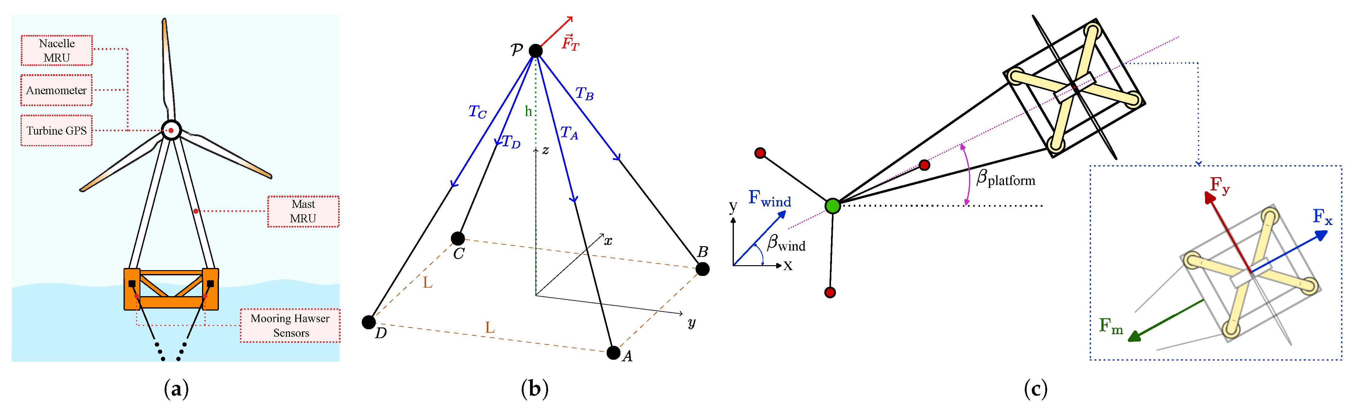
2. Eolink Floating Wind Turbine Concept

Figure 1a presents the front view of the design of Eolink’s floating wind turbine, and more detailed figures can be found in [6]. In contrast to conventional configurations that use a single tower, this design employs four distinct pillars that connect the turbine structure to the corners of the floating platform, as described in Figure 1b. As described in [8], this configuration yields a more uniform stress distribution, reduced dynamic vibration, a smaller platform footprint, and lower initial investment costs. The pyramid-shaped support base distributes the rotor’s mass evenly between bearings at both ends, enabling a lighter nacelle and the use of four slender supports instead of a single monolithic pole. At a 5-MW scale, the platform measures approximately 50 m in length and 50 m in width, with a hub height of about 100 m supporting a rotor diameter of 140 m. Furthermore, the platform’s structural robustness and hydrodynamic stability allow it to accommodate turbines exceeding 10 MW at full scale.

The turbine is engineered to naturally align with the wind via a front-mounted tether, as depicted in Figure 1c. Although wind direction and ocean currents are generally aligned in deep-water conditions, the design incorporates a dynamic ballast system capable of adjusting the turbine orientation by up to 120° to manage any misalignment. The floating platform is attached to the seabed using three anchor lines (red dots in Figure 1c), all of them connected to the rotating buoy (green dot in Figure 1c). The buoy contains all the mechanical rotating equipment necessary to achieve effective weathervaning. This system also enables load mitigation by decoupling the platform’s motion from its mooring system. In a simplified top-view representation, when the platform weathervanes to align with the wind force ($F_{\mathrm{wind}}$) coming from a direction ${\beta }_{\mathrm{wind}}$, it experiences resulting forces in the surge ($F_x$) and sway ($F_y$) directions. These forces displace the turbine from its initial position, while the mooring system provides a restoring force ($F_m$) to maintain platform stability. The available power output of the floating offshore wind turbine (FOWT) depends on its alignment with the wind direction, expressed as $P_{\mathrm{av}}=f({\beta }_{\mathrm{platform}},{\beta }_{\mathrm{wind}})$. When misaligned (i.e., ${\beta }_{\mathrm{platform}}\ne {\beta }_{\mathrm{wind}}$), the turbine produces less power than in the aligned condition (i.e., ${\beta }_{\mathrm{platform}}={\beta }_{\mathrm{wind}}$). This effect is discussed in more detail in the following sections.

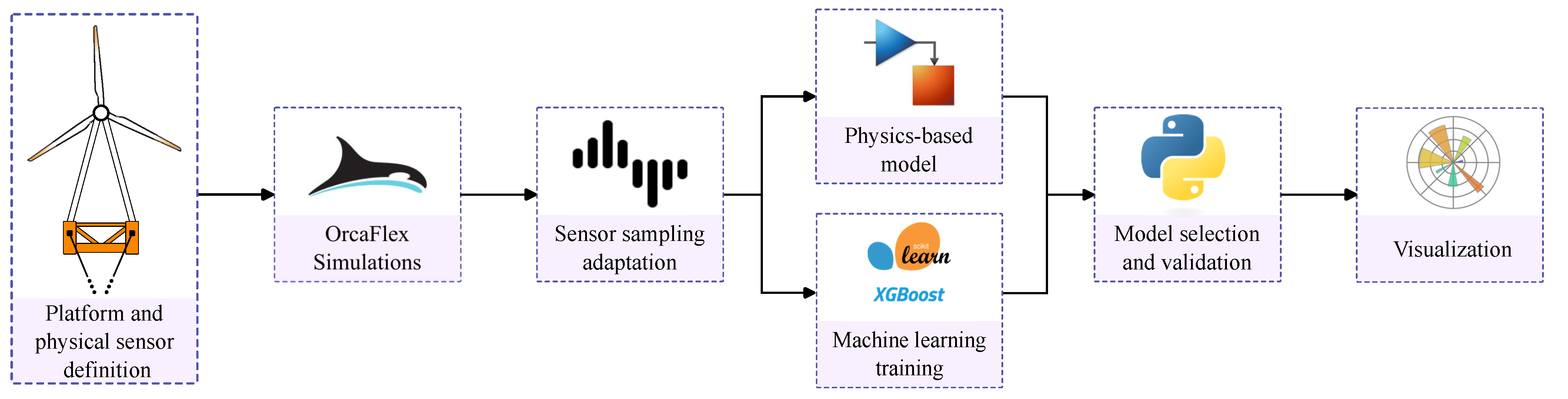
3. Methods and Design of the Virtual Sensors

3.1. Methodology

The development of virtual sensors for floating offshore wind platforms follows a structured pipeline, as illustrated in Figure 2. The process begins with the definition of the platform configuration and physical sensor layout, which provides the basis for subsequent simulation and modeling. High-fidelity dynamic responses are then generated using OrcaFlex 11.5 simulations, incorporating the relevant environmental and operational conditions. To ensure compatibility with real-world measurement systems, the synthetic data is adapted to match the sampling characteristics of the onboard physical sensors. The processed data is used to develop two parallel models—a physics-based model in Simulink and machine learning models trained with scikit-learn and xgboost. These two models are later integrated into a PIML (physics-informed machine learning) framework during the training and model selection phase, where optimal configurations are selected based on accuracy and generalization performance. Finally, the trained virtual sensor is validated against reference data, and its performance is visualized.

3.2. Assumptions of Physical Sensors Installed

In the initial phase of developing virtual sensors, the first step is to identify which physical sensor measurements can serve as effective input features. Although detailed guidelines on sensor placement for floating wind turbine designs are limited, several sensor technologies are generally assumed to be integrated into these systems. Wind speed and direction are typically measured using anemometers and/or wind LiDAR systems, while variables related to wave elevation, wave direction, current velocity, and direction can be captured by wave buoys or radar-based instruments. Structural health monitoring can be obtained by installing accelerometers to record dynamic motions and strain gauges to detect elastic deformations in key structural components. Global Positioning System (GPS) sensors are installed to precisely track the platform’s location and movement, together with inertial measurement units (IMUs) for assessing orientation and tilt. Apart from that, it is assumed that all rotor nacelle assembly (RNA) components of the wind turbine, generator, and related systems are equipped with standard sensor placements (e.g., accelerometers for vibration monitoring, temperature sensors for thermal regulation, etc.). The used system and its associated sampling frequencies are presented in

Table 2. Sampling frequencies of the sensors used in the study.

Physical Sensor	Sample Frequency	Unit
Anemometer	1	Hz
GPS	1	Hz
Mooring Tension	5	Hz
Mast/Nacelle MRU	10	Hz
Wave-Current Data	Constant	–

.

3.3. Load Cases in OrcaFlex and Data Analysis

Table 3. Summary of simulated load cases used in the dynamic analysis with OrcaFlex.

Case	Turbine Condition	Wind Model	Wave Model	Current Model	Misalignment
1	Operational	Turbulent 7 m/s	$H_s$ = 1.0 m, $T_p$ = 5 s	Constant 0.1 m/s	No
2	Operational	Turbulent 11 m/s	$H_s$ = 2.5 m, $T_p$ = 6 s	Constant 0.2 m/s	Yes
3	Operational	Turbulent 15 m/s	$H_s$ = 3.5 m, $T_p$ = 7.5 s	Constant 0.2 m/s	No
4	Operational	Turbulent 9 m/s	$H_s$ = 1.8 m, $T_p$ = 5.5 s	Constant 0.1 m/s	No
5	Operational	Turbulent 13 m/s	$H_s$ = 3.0 m, $T_p$ = 7 s	Constant 0.2 m/s	Yes
6	Operational	Dir. change at 9 m/s	$H_s$ = 2.0 m, $T_p$ = 5.5 s	Constant 0.1 m/s	Yes
7	Operational	Dir. change at 13 m/s	$H_s$ = 3.0 m, $T_p$ = 7 s	Constant 0.2 m/s	Yes
8	Operational	Step gust to 25 m/s	$H_s$ = 4.0 m, $T_p$ = 8 s	Constant 0.3 m/s	No
9	Idling (Storm)	Steady 25 m/s	$H_s$ = 6.0 m, $T_p$ = 10 s	Constant 0.6 m/s	Yes
10	Parked (Survival)	Extreme wind (50-year)	$H_s$ = 8.0 m, $T_p$ = 12 s	Constant 0.9 m/s	Yes
11	Parked (Survival)	No wind	$H_s$ = 10.0 m, $T_p$ = 15 s	Constant 0.9 m/s	No

summarizes the load cases defined for the dynamic analysis performed with OrcaFlex at full scale. These cases include different turbine states, such as operational, idling, and parked (survival), under varying environmental conditions. Wind inputs include steady, turbulent, directional-change, and step-gust conditions, with mean speeds ranging from below-rated conditions up to extreme 50-year return values. Wave conditions are described by significant wave height ($H_s$) and peak period ($T_p$), covering realistic mild to severe sea states consistent with wind intensity. Currents are modeled as steady and unidirectional, with magnitudes ranging from 0.1 m/s to 0.9 m/s, aligned with each case’s severity. Selected cases include wind–wave–current misalignment to evaluate its influence on the system’s dynamic response.

First, to determine which measurements can serve as inputs for the design of the virtual sensors, we need to identify the correlated variables. The correlations were calculated using the Spearman correlation method. Figure 3 shows the five most correlated features for each desired target. Note that the strongest correlation coefficients are those closest to 1 or −1.

As can be seen in the green lower side box, the force in the right hawser exposes the highest correlation with the forces in the other hawser, as can be easily understood. However, this variable will not be taken into account, since we are neglecting the installation of a physical sensor there. Next, we can see correlations with wind speed and direction, as these factors directly influence the aerodynamic loads on the wind turbine. As wind speed increases, so does the magnitude of the force transmitted through the turbine through the floater into the mooring system, giving a reaction. Similarly, changes in wind direction alter the distribution of these forces along the hawsers. Additionally, surging exhibits a high correlation, followed by the swaying of the structure. The presence of these mooring-related features is expected, especially in surging, as observed in other floating wind substructures.

On the other hand, the variables most correlated to the bending moment at the top of the pyramidal wind structure are depicted in the purple upper-side box. Aerodynamic thrust tends to appear since it directly generates bending and torsional forces, while the load transmitted through the masts adds to these moments. The forces in the upwind masts appear, as expected, to be linked to the forces at the connection between the substructure and the nacelle. The platform pitch probably appears due to altering the effective load distribution, affecting the lever arm of these forces. Additionally, the appearance of control parameters such as blade pitch and rotor speed is believed to be related to the need to adjust aerodynamic loads and regulate power, thereby influencing the overall moment at the top.

Following these two findings, a simplified scheme of the virtual sensors is introduced in Figure 4. We propose the following objectives: The first objective is to design a virtual sensor (VS1) for one of the hawsers in the mooring system, aiming to avoid the installation of sensors underwater. The input features for this sensor include wind speed, wind direction, and, if needed, surge, as elements of $X_3$. Since the forces are highly correlated, the output of the first virtual sensor ($F_{\mathrm{hawser}1}$) is later used to calculate the tension in the other hawser ($F_{\mathrm{hawser}2}$). In this way, the sensor estimates the force in both of the mooring hawsers. The last objective is to develop another virtual sensor (VS3) to estimate the top masts’ bending moment ($B{M}_{\mathrm{masts}}$) based on aerodynamic thrust forces, platform pitch dynamics, and the torque. Additionally, the inclusion of control parameters such as pitch angle and rotor angular velocity will be evaluated in a subsequent phase.

Although the virtual sensors presented here are designed using supervised machine learning models trained on a wide range of the floating platform’s behaviors, it is important to note that a method for integrating physics-based constraints into the supervised machine learning models will be introduced later in this paper, to avoid relying just on data-driven algorithms and to enable comparisons. Therefore, let us firstly introduce the main equations defining the dynamics of the platform, and later, the supervised machine learning algorithms used.

3.4. Physics Relations for PIML Integration

The simplified model used in the physics-informed algorithms includes key environmental loads and mooring constraints acting on the floating offshore wind turbine (FOWT). As previously discussed and depicted in Figure 1, the platform exhibits weathervaning behavior and must be modeled with six degrees of freedom (6DOF): surge, sway, heave, roll, pitch, and yaw. Two hawsers connect selected columns of the platform to a buoy, which is anchored to the seabed using three mooring lines. The environmental loads considered include aerodynamic forces from wind, hydrodynamic forces from waves and steady currents, and hydrostatic restoring forces resulting from buoyancy and gravity.

The platform dynamics are governed by the Newton–Euler equations, incorporating added mass and hydrodynamic damping from OrcaWave, along with restoring forces derived from hydrostatics and the mooring system. The equations can be expressed in a generalized coordinate system, where $\mathbf{q}=\left[\begin{array}{c}\mathit{x};\mathsf{\eta }\end{array}\right]$ is the generalized position vector, including translational ($\mathit{x}$) and rotational ($\mathsf{\eta }$) coordinates, and $\dot{\mathbf{q}}=\left[\begin{array}{c}\dot{\mathit{x}};\mathsf{\omega }\end{array}\right]$ is the generalized velocity vector. The system’s dynamics are governed by a generalized mass-inertia matrix, added mass, damping, and restoring forces. The equation of motion is as follows:

$$(\mathbf{M}+\mathbf{A})\ddot{\mathbf{q}}+\mathbf{B}\dot{\mathbf{q}}+\mathbf{C}\mathbf{q}+\left[\begin{array}{c}0\\ \omega \times \left((\mathbf{I}+{\mathbf{A}}_{\theta })\omega \right)\end{array}\right]=\mathbf{\tau }$$

(1)

where $\mathbf{M}$ is the global mass-inertia matrix, $\mathbf{A}$ is the added mass and added inertia matrix, $\mathbf{B}$ represents hydrodynamic and rotational damping, and $\mathbf{C}$ is the restoring force and moment matrix. The nonlinear gyroscopic term $\omega \times \left((\mathbf{I}+{\mathbf{A}}_{\theta })\omega \right)$ appears only in the rotational part of the equation. The generalized external force vector is given by the aerodynamic, hydrodynamic, and mooring forces and moments:

$$\mathbf{\tau }=\left[\begin{array}{c}{\mathbf{F}}_{\mathrm{aero}}+{\mathbf{F}}_{\mathrm{hydro}}+{\mathbf{F}}_{\mathrm{m}}\\ {\mathbf{M}}_{\mathrm{aero}}+{\mathbf{M}}_{\mathrm{hydro}}+{\mathbf{M}}_{\mathrm{m}}.\end{array}\right]$$

(2)

The aerodynamic loads depend on the exposed surfaces of the structure and the relative alignment between the platform and the wind. For each of the j structural components, the aerodynamic force and moment contributions are modeled as follows:

$$\begin{array}{cc}\hfill {\mathbf{F}}_{aero,j}& =0.5{\rho }_a{C}_{D,j}{A}_{e,j}{U}^2{\mathbf{n}}_j,\hfill \end{array}$$

(3)

$$\begin{array}{cc}\hfill {\mathbf{M}}_{aero,j}& =0.5{\rho }_a{C}_{M,j}{A}_{e,j}{U}^2{\mathbf{r}}_{a,j},\hfill \end{array}$$

(4)

where ${\rho }_a$ is the air density, $C_{D,j}$ and $C_{M,j}$ are the drag and moment coefficients for component j, $A_{e,j}$ is its effective projected area (which is a function of the platform’s orientation relative to the wind), ${\mathbf{n}}_j$ is the unit vector in the effective wind direction for component j, and ${\mathbf{r}}_{a,j}$ is the lever arm from the center of gravity (CG) to the center of force application on component j. The aerodynamic coefficients $C_{D,j}$ and $C_{M,j}$ vary depending on the flow regime and angle of attack ${\alpha }_j$. For the different components (e.g., rotor, masts, etc.), these coefficients are functions of different Reynolds numbers, ${\mathrm{Re}}_j=f({\rho }_a,U,L_j,{\mu }_a)$, where $L_j$ is a characteristic length of the component and ${\mu }_a$ is the air’s dynamic viscosity. The angle of attack ${\alpha }_j$ is the angle between the wind direction and the reference axis of the component. Changes in ${\alpha }_j$ alter the pressure distribution over the surface, influencing both drag and lift forces.

The mast’s structure has been modeled as a pyramidal truss subjected to a horizontal wind load (relative to the prevailing wind direction) applied by the turbine at the top node. The equilibrium of the structure is determined by decomposing the forces into components along the coordinate axes, using unit vectors to represent the direction of each mast and its corresponding force. These forces are balanced at the top node, where the turbine’s thrust force is applied. The internal forces along the masts are treated as axial forces, and the structure is assumed to be in a state of static equilibrium with no external moments except for the applied wind force. Following the scheme introduced in Figure 1b, each mast connects the top node, given by $\mathcal{P}=(0,0,h)$, to a base node of the square-shaped floater. Given a side length $L_m=\parallel {\overrightarrow{r}}_i\parallel =\sqrt{2a^2+h^2}$, let $a=L_m/2$ and define the base nodes as $A=(a,a,0)$, $B=(-a,a,0)$, $C=(-a,-a,0)$, $D=(a,-a,0)$, so the vectors from the top node $\mathcal{P}$ to the base nodes are

$${\overrightarrow{r}}_A=\left(\begin{array}{c}a\\ a\\ -h\end{array}\right),{\overrightarrow{r}}_B=\left(\begin{array}{c}-a\\ a\\ -h\end{array}\right),{\overrightarrow{r}}_C=\left(\begin{array}{c}-a\\ -a\\ -h\end{array}\right),{\overrightarrow{r}}_D=\left(\begin{array}{c}a\\ -a\\ -h\end{array}\right).$$

(5)

while the unit vectors along the masts are defined by ${\mathbf{u}}_i={\overrightarrow{r}}_i/L_m$ being $i=A,B,C,D$. Following the scheme in Figure 1b, and assuming that the thrust force of the wind turbine, given by Equation (9) is applied at $\mathcal{P}$ and acts in the positive x-direction, the wind load vector becomes ${\mathbf{F}}_w=(F_{\mathrm{T}},0,0)$. Next, let $T_i$ be the internal force in the mast joining $\mathcal{P}$ to node i (with positive values indicating tension). Then, the equilibrium at the top node $\mathcal{P}$ is given by

$${\mathbf{F}}_w+\sum _{i=A}^D{T}_i{\mathbf{u}}_i=\mathbf{0}.$$

(6)

Since at each base node i, the reaction is given by the force transmitted through the corresponding mast, ${\mathbf{R}}_i=T_i{\mathbf{u}}_i$, structure is given by

$${\mathbf{F}}_w+\sum _{i=A}^D{\mathbf{R}}_i=\mathbf{0}.$$

(7)

Moreover, taking moments about the origin into account yields

$${\mathbf{r}}_{\mathcal{P}}\times {\mathbf{F}}_w+\sum _{i=A}^D{\mathbf{r}}_i\times {\mathbf{R}}_i=\mathbf{0},$$

(8)

where ${\mathbf{r}}_{\mathcal{P}}$ is the position vector of the top node $\mathcal{P}$.

Finally, for the rotor, we considered that the thrust force, determined at the height of the top of the masts h as depicted in Figure 1, is influenced by the platform’s pitching rate, ${\dot{\theta }}_p$. This yields

$$F_T=0.5{\rho }_a\pi R^2{C}_T\left({\displaystyle \frac{{\omega }_{r}R}{U_r}},\beta \right){(U-h{\dot{\theta }}_p)}^2,$$

(9)

where $\rho$ is the air density, R denotes the rotor diameter, $C_T$ denotes the thrust coefficient, which is a function of the tip speed ratio (characterized by the rotor speed ${\omega }_r$) and the blade pitch angle $\beta$. Since the floating platform does not apply active yaw control, yawing is achieved exclusively through adjustments in blade pitch. Note that the same strategy is also employed in the OrcaFlex model. Generator torque control is employed to regulate the turbine’s rotational speed, ensuring a stable power output, which in fact depends on both wind speed and platform misalignment as

$$P_{av}=0.5{\rho }_a{\mathcal{C}}_p\left(\alpha \right)A{U}^{3}cos(\Delta \beta ).$$

(10)

where $\Delta \beta ={\beta }_{\mathrm{platform}}-{\beta }_{\mathrm{wind}}$, as depicted in Figure 1c.

The hydromechanics analysis was carried out to evaluate the forces and moments applied to the floating platform in all six degrees of freedom (surge, sway, heave, pitch, roll, and heave). In general, hydromechanics can be split into hydrostatics and hydrodynamics. Hydrostatics, such as buoyancy forces, contribute to restoring forces that let the structure float upright. On the other hand, hydrodynamics are mainly influenced by the dynamic wave environment and are used to calculate the forces impacting the structure. As this is a reduced-order model, the submerged and surface-piercing parts are simplified as cylindrical slender columns, enabling the use of Morison’s equation. Considering the columns’ geometry, directional effects of waves and their relative local velocity, the hydrodynamic force on the arc length s of a submerged part was calculated as follows:

$$d{\mathbf{F}}_{hydro}\left(s\right)=0.5{\rho }_w{C}_D\left(s\right)D\left(s\right)\left|\mathbf{u}\left(s\right)\right|\mathbf{u}\left(s\right)ds+{\rho }_w{C}_M\left(s\right){\displaystyle \frac{\pi D{\left(s\right)}^2}{4}}{\displaystyle \frac{d\mathbf{u}\left(s\right)}{dt}}ds,$$

(11)

where ${\rho }_w$ is the water density, $C_D\left(s\right)$ and $C_M\left(s\right)$ are local drag and inertia coefficients, $D\left(s\right)$ is the local diameter of the element, and $\mathbf{u}\left(s\right)$ is the local velocity due to waves with its associated direction. Integrating Equation (11) over the wet surface gives the total wave-induced force. The hydromechanics analysis was conducted in OrcaFlex, and the results were extracted using look-up tables for the development of the virtual sensors. Finally, each mooring line, whether a hawser from the platform to the buoy or an anchor line from the buoy to the seabed, is assumed to follow a static catenary profile. The position vector along the mooring line part i is given by

$${\mathbf{r}}_i\left(s\right)={\left[\begin{array}{cc}{x}_i\left(s\right)& z_i\left(s\right)\end{array}\right]}^{\mathsf{T}},i=1,\dots ,5,$$

(12)

where s denotes the arc length, $x_i\left(s\right)$ denotes the horizontal coordinate, and $z_i\left(s\right)$ denotes the vertical coordinate (with $z>0$ defined downward). The local equilibrium is expressed as follows:

$${\displaystyle \frac{d}{ds}}{\mathbf{T}}_i\left(s\right)+{\rho }_{i}g{\mathbf{e}}_z=\mathbf{0},$$

(13)

with ${\mathbf{T}}_i\left(s\right)={\left[\begin{array}{cc}{T}_{x,i}\left(s\right)& T_{z,i}\left(s\right)\end{array}\right]}^{\mathsf{T}}$ being the tension vector, ${\rho }_i$ the linear mass density, g the gravitational acceleration, and ${\mathbf{e}}_z={\left[\begin{array}{cc}0& 1\end{array}\right]}^{\mathsf{T}}$ the vertical unit vector. Assuming a constant horizontal tension $T_{0,i}$ at the connection point, and an initial inclination ${\theta }_i$, the catenary profile is given by

$$z_i\left(x\right)={\displaystyle \frac{T_{0,i}sin{\theta }_i}{{\rho }_{i}g}}cosh\left({\displaystyle \frac{{\rho }_{i}g}{T_{0,i}sin{\theta }_i}}x\right)-{\displaystyle \frac{T_{0,i}sin{\theta }_i}{{\rho }_{i}g}}.$$

(14)

At the catenary anchor leg mooring, the resultant forces from the two hawsers ($i=1,2$) and the three anchor lines ($i=3,4,5$) must counterbalance the environmental loads acting on the platform, ${\mathbf{F}}_{env}^{\left(p\right)}$ as

$$\sum _{i=1}^5{\mathbf{T}}_i+{\mathbf{F}}_{env}^{\left(p\right)}=\mathbf{0},$$

(15)

where each line’s force is given by ${\mathbf{T}}_i=T_{0,i}{\left[\begin{array}{cc}cos{\theta }_i& sin{\theta }_i\end{array}\right]}^{\mathsf{T}}$. Based on the previous relation, the two hawsers connecting the platform at attachment points ${\mathbf{r}}_1^{\left(p\right)}$ and ${\mathbf{r}}_2^{\left(p\right)}$ will define the total net mooring force draw in Figure 1c and the resulting moment about the center of gravity (CG) as

$$\begin{array}{cc}\hfill {\mathbf{F}}_m& ={\mathbf{T}}_1+{\mathbf{T}}_2,\hfill \end{array}$$

(16)

$$\begin{array}{cc}\hfill {\mathbf{M}}_m& ={\mathbf{r}}_1^{\left(p\right)}\times {\mathbf{T}}_1+{\mathbf{r}}_2^{\left(p\right)}\times {\mathbf{T}}_2.\hfill \end{array}$$

(17)

The previous relation is valid for the operation of the platform when it is aligned with the wind. In the case of misalignment, a correction is applied to the surge, sway, and yaw components of ${\mathbf{F}}_m$ and ${\mathbf{M}}_m$ as a function of ${\beta }_{\mathrm{platform}}$ and ${\beta }_{\mathrm{wind}}$, similar to Equation (10).

3.5. Supervised and Physics-Informed Machine Learning

This study applies two supervised learning techniques—random forest (RF) and gradient boosting—specifically using the XGBoost implementation. Both models are ensemble-based and operate by aggregating the predictions of multiple decision trees. They are well-suited for scenarios involving non-linear relationships, moderate data sizes, and limited computational resources. In practice, both methods are readily accessible through Python 3.11 libraries such as scikit-learn and xgboost, offering efficient training procedures, built-in cross-validation, and compatibility with common data preprocessing pipelines.

Random forest constructs a set of M decision trees, each trained on a randomly resampled subset of the original training data. The final prediction for a sample x is calculated by averaging the outputs of all trees:

$$f\left(x\right)={\displaystyle \frac{1}{M}}\sum _{m=1}^M{f}_m\left(x\right),$$

(18)

where $f_m\left(x\right)$ represents the output of the m-th tree. This method reduces overfitting by decreasing the variance of individual learners.

Gradient boosting is implemented via XGBoost, a widely used and optimized framework that enhances the traditional boosting algorithm by introducing regularization and efficient tree construction strategies [24]. In this method, models are trained sequentially, with each new tree correcting the residual errors of the existing ensemble. Let $\mathcal{L}(y,\widehat{y})$ be a convex and differentiable loss function that quantifies the difference between the observed target y and the predicted value $\widehat{y}$. The prediction at iteration t is updated as follows:

$${\widehat{y}}_i^{\left(t\right)}={\widehat{y}}_i^{(t-1)}+\eta g_t\left(x_i\right),$$

(19)

where $\eta$ is the learning rate and $g_t\left(x\right)$ is the decision tree fitted to the pseudo-residuals, defined as follows:

$$r_i^{\left(t\right)}=-{\left.{\displaystyle \frac{\partial \mathcal{L}(y_i,{\widehat{y}}_i)}{\partial {\widehat{y}}_i}}\right|}_{{\widehat{y}}_i={\widehat{y}}_i^{(t-1)}}.$$

(20)

This iterative approach allows the model to improve its predictive accuracy while managing complexity through built-in regularization.

In addition to purely data-driven modeling, a physics-informed machine learning approach is implemented to incorporate prior physical knowledge into the virtual sensing framework. The reduced-order physics-based model implemented in Simulink is used to generate approximate estimates of the target quantity, denoted as $y_{\mathrm{ph},i}$. These estimates are not used as direct labels, but rather serve as a reference for enforcing physical consistency. Since the employed machine learning models are ensemble-based and non-differentiable, the physics-based term cannot be directly incorporated into a gradient-based loss function. Instead, the PIML integration is realized by constructing an augmented training process in which both the measured output $y_i$ and the physics-based output $y_{\mathrm{ph},i}$ are used to evaluate the model’s consistency. Specifically, after initial training using standard supervised learning on available data, the predicted output ${\widehat{y}}_i$ is compared against both the ground truth and the physics-based reference. A composite evaluation metric is defined as

$${\mathcal{L}}_{\mathrm{total}}=\sum _{i=1}^n\left[\mathcal{L}(y_i,{\widehat{y}}_i)+\lambda {\mathcal{L}}_{\mathrm{ph}}({\widehat{y}}_i,y_{\mathrm{ph},i})\right],$$

(21)

where $\mathcal{L}(y_i,{\widehat{y}}_i)$ denotes the data-driven prediction error, ${\mathcal{L}}_{\mathrm{ph}}({\widehat{y}}_i,y_{\mathrm{ph},i})$ quantifies the deviation from the Simulink-based physics estimate, and $\lambda \in [0,1]$ controls the relative importance of the physics term. This formulation is applied during model selection and tuning rather than during training itself. By incorporating the physics output as an auxiliary consistency check, the framework helps identify models that not only fit the data well but also remain physically plausible.

4. Results

To assess the performance of the proposed approach, the results are presented based on the workflow illustrated in Figure 2 and the load cases described in Table 3. The analysis was conducted using an OrcaFlex output dataset containing 46 features and 156,009 entries, providing sufficient data for the application of supervised machine learning techniques. The input time series for wind and wave conditions were generated using TurbSim and the JONSWAP spectrum, respectively.

For the machine learning models, hyperparameter optimization was performed using automated grid and random search methods combined with k-fold cross-validation. This process was used to identify suitable values for maximum tree depth, minimum samples per split, the number of estimators, and learning rate. Subsequent sensitivity analyses were carried out to evaluate the influence of these parameters on model performance. Final parameter values were selected based on their ability to minimize cross-validated error metrics. The corresponding results are presented in this section. It should be noted that the study focuses on specific time intervals influenced by varying environmental conditions, which are particularly relevant for this type of technology.

Section 4 is divided into two main parts. Section 4.1 presents the mooring hawser forces, including both VS1 and VS2 outputs. This analysis considers different environmental conditions and turbine operating states, including below-rated and near-rated wind speeds. Section 4.2 addresses the bending moment response, evaluated under wind conditions near the rated operating point. Each subsection provides the necessary structure for understanding the performance of the corresponding virtual sensor.

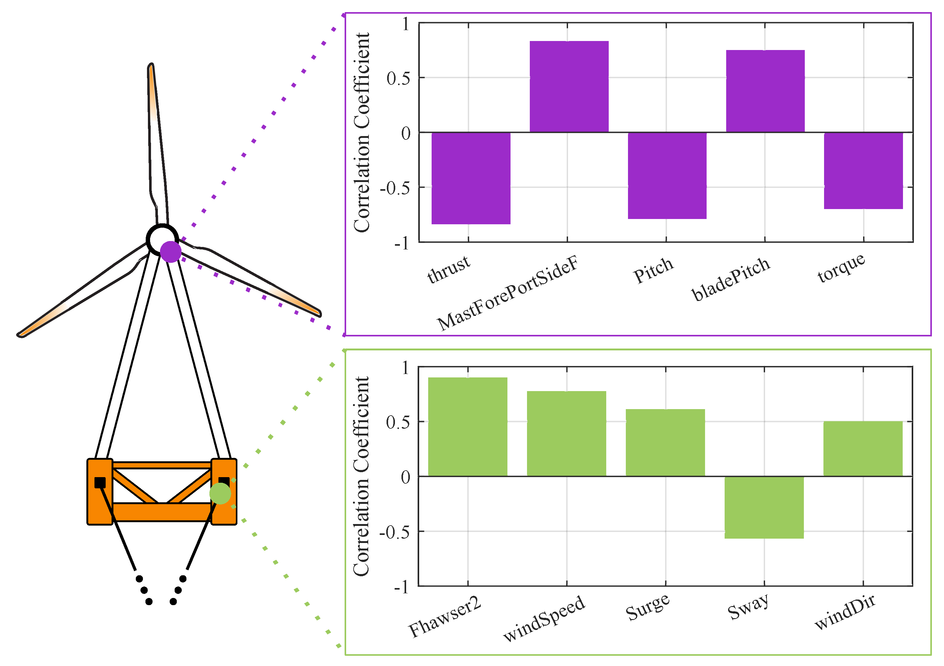
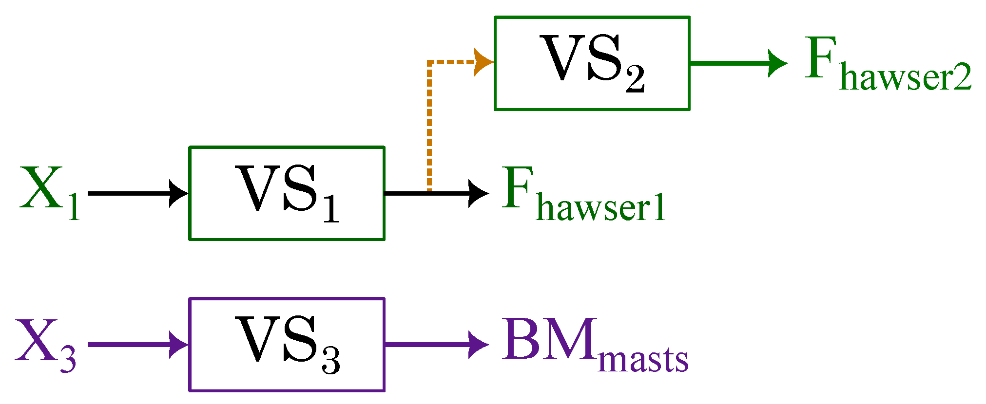
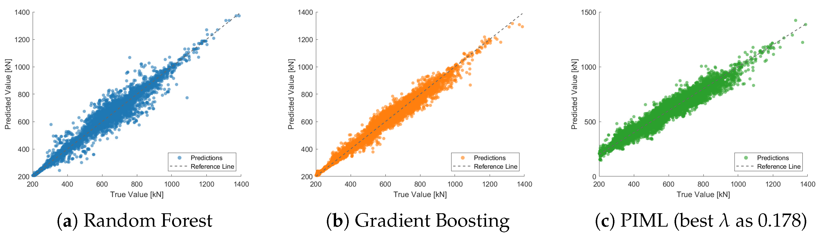
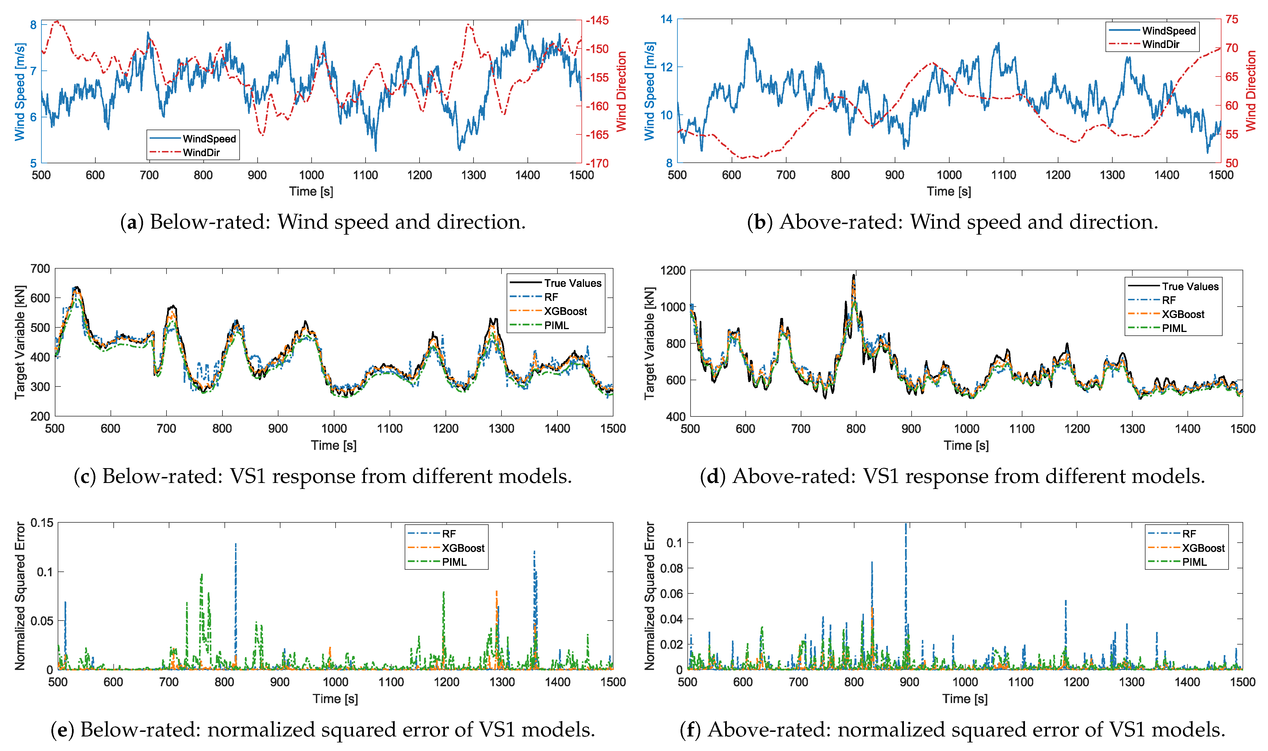
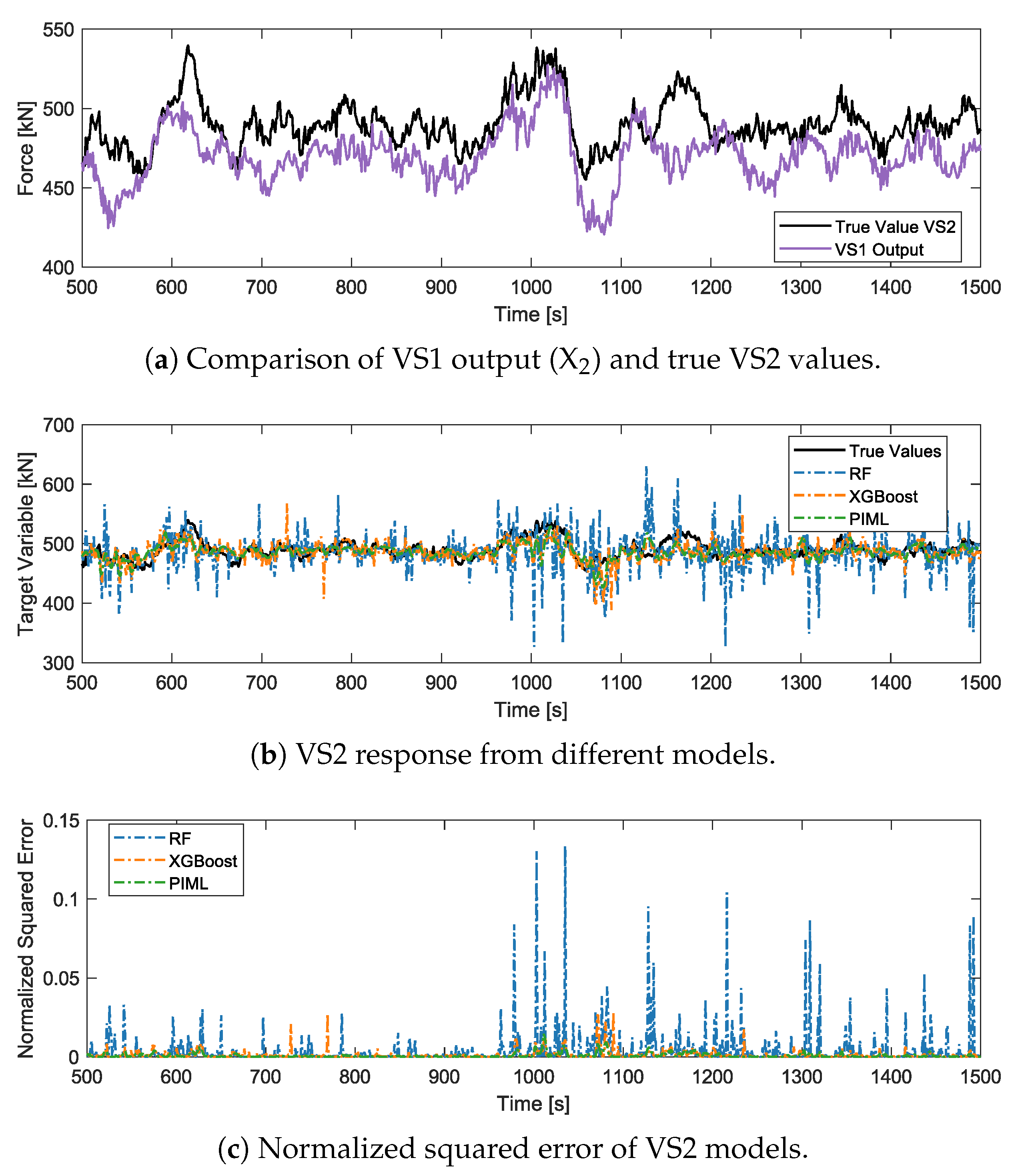
4.1. Mooring Hawsers

This subsection presents the results from the virtual sensors associated with the mooring hawsers, VS1 and VS2. Specifically, we first evaluate predictions for the right mooring hawser, designated as VS1 and shown in Figure 3. The tests are conducted under below-rated conditions, incorporating a progressive and varying wind direction change, combined with misaligned wave and current conditions. This scenario was selected because varying wind directions significantly influence the weathervaning behavior and, consequently, the performance of the mooring system. The analysis begins with the assessment of regression results to quantify the accuracy of each prediction algorithm. Subsequently, time series data are presented to evaluate the performance of the VS1 model in the time domain under two distinct scenarios—one under rated conditions and the other under above-rated conditions.

The initial evaluation of the virtual sensor performance for the mooring hawsers was conducted under aligned wind, wave, and current conditions, with environmental directions from the west. Figure 5 illustrates the regression results obtained after training virtual sensor 1 (VS1) using three machine learning methods to predict tensions in hawser 1. Specifically, subfigure (a) shows the random forest predictions, subfigure (b) presents the gradient boosting (XGBoost) algorithm results, and subfigure (c) displays outcomes from the physics-informed machine learning (PIML) model, optimized with $\lambda =0.178$.

Model performance was evaluated using mean squared error (MSE), root mean squared error (RMSE), mean absolute error (MAE), and the coefficient of determination ($R^2$).

Among the tested models, XGBoost exhibited the highest predictive accuracy, with an MSE of 275.81, RMSE of 16.61, MAE of 12.65, and an $R^2$ value of 0.9815. The PIML approach demonstrated strong performance as well, ranking second with an MSE of 380.44, RMSE of 19.50, MAE of 13.31, and $R^2$ of 0.9783. The random forest method showed comparatively lower accuracy, yielding an MSE of 753.25, RMSE of 27.45, MAE of 19.91, and an $R^2$ of 0.9668. The high $R^2$ values across all models indicate robust predictive capabilities using the selected inputs of

Table 4. Characteristics of the input vectors for each virtual sensor.

Input Vector	Variables	Sample Frequency	Output
X1	Wind Speed Signal	1 Hz	Fhawser1
	Latitude/Longitude	1 Hz
	Platform Surge	10 Hz
X2	Fhawser1	5 Hz	Fhawser2
X3	Wind Speed Signal	1 Hz	BMmasts
	Torque	1 Hz
	Platform Pitch	10 Hz

, validating the effectiveness of the selected input variables and machine learning techniques for accurately estimating tensions in mooring hawsers. Figure 6 shows the time series validation of virtual sensor VS1 under two operational scenarios—below-rated conditions (left column) and above-rated conditions (right column). Each column contains three subplots—wind speed and direction (top row), model predictions and reference tensions (middle row), and normalized squared error of each model (bottom row). A 1000-s interval is displayed in each subplot.

Under below-rated conditions (Figure 6a,c,e), the average wind speed is approximately 7 m/s, predominantly from the west with a mean direction of −155°. Under above-rated conditions (Figure 6b,d,f), the wind speed increases to an average of 11 m/s, predominantly from the northeast at an average direction of 60°.

The middle plots (Figure 6c,d) compare the predicted tensions from the random forest (RF), gradient boosting (XGBoost), and physics-informed machine learning (PIML) models against the OrcaFlex reference data (black line). All three models closely track the reference data across both operating conditions.

The lower plots (Figure 6e,f) depict the normalized squared error (NSE) for each model. XGBoost exhibits the lowest error consistently across both scenarios. The PIML model also performs effectively, although it occasionally exhibits higher error peaks. In general, random forest shows the largest deviations, especially during transient events. Time series results validate the accuracy of the virtual sensor models in estimating hawser tensions under varying environmental conditions.

Figure 7 presents the regression scores for virtual sensor 2 (VS2), designed to predict tensions in the second mooring hawser. Figure 7a–c illustrate the performance of the random forest, XGBoost, and PIML methods, respectively. For the PIML model, the optimal $\lambda$ was determined to be 0.674, indicating substantial reliance on physics-based modeling components. The regression plots highlight the differences in predictive performance. The random forest method (Figure 7a) displays significant dispersion from the reference line, reflected by a relatively low $R^2$ (0.8132), high MSE (6078.44), RMSE (77.96), and MAE (37.60). This suggests that purely data-driven methods have limitations in accurately capturing complex dynamics when input variables are scarce. In contrast, the PIML model (Figure 7c) achieves an improved accuracy with a higher $R^2$ (0.9342), and significantly lower MSE (2790.91), RMSE (47.21), and MAE (30.24). Gradient boosting performs moderately between these extremes, showing better results than random forest but slightly inferior compared to the PIML method.

Figure 8 provides the insights by analyzing these models through time series predictions. Figure 8a presents the force output from VS1 (used here as input for VS2, see Table 4), against the true VS2 tensions obtained from OrcaFlex. The discrepancy between the two series indicates distinct dynamics between the hawsers. Thus, relying exclusively on data-driven models, which may inadvertently incorporate signals from a related but dynamically different hawser (such as VS1), can lead to erroneous predictions.

Figure 8b compares the predicted time series from each modeling approach against true tension values. The random forest model notably misinterprets the dynamics, exhibiting errors when transient changes occur, as shown between 1000 and 1100 s. Figure 8c, displaying normalized squared errors, further emphasizes these inaccuracies. The hybrid PIML model significantly reduces these errors by incorporating physics-based corrections, as evidenced by fewer and smaller peaks in its error signal.

These analyses demonstrate that, despite data-driven models such as random forest and gradient boosting performing strongly for certain applications, PIML approaches are particularly beneficial when input data is limited or potentially misleading. The optimal higher value of $\lambda$ (0.674) confirms the PIML model’s increased reliance on the physics-based component, improving its robustness and accuracy in complex prediction tasks involving coupled but distinct dynamic systems.

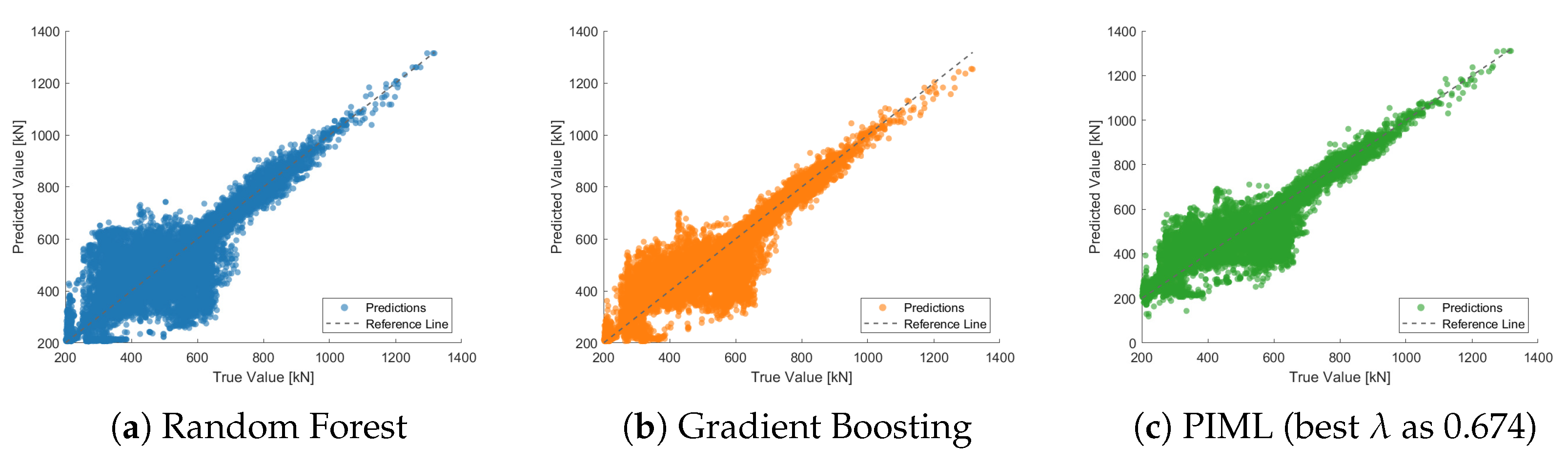
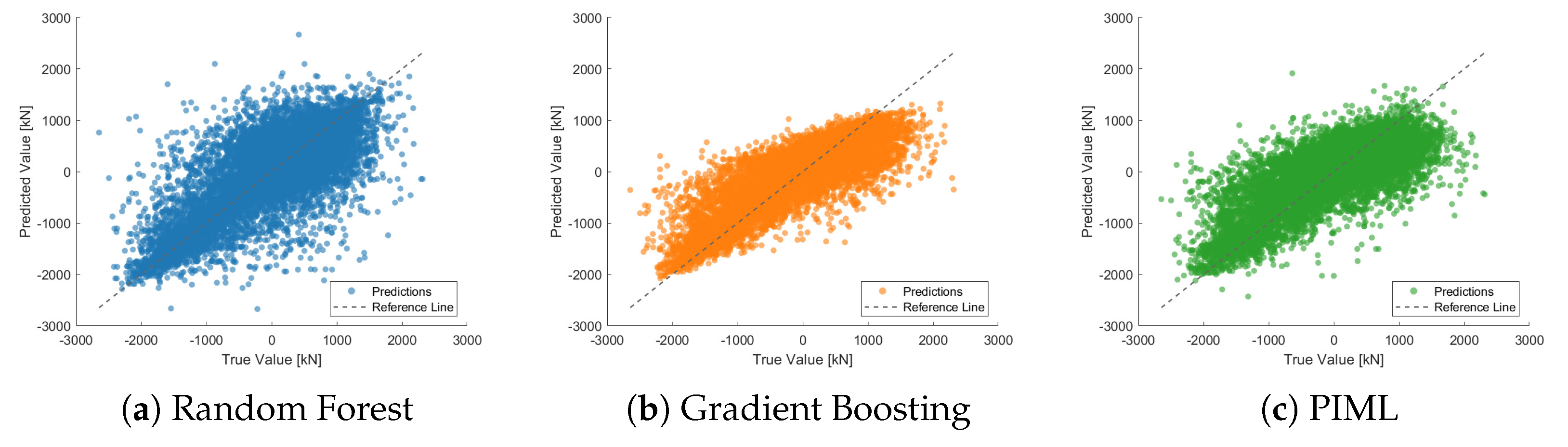
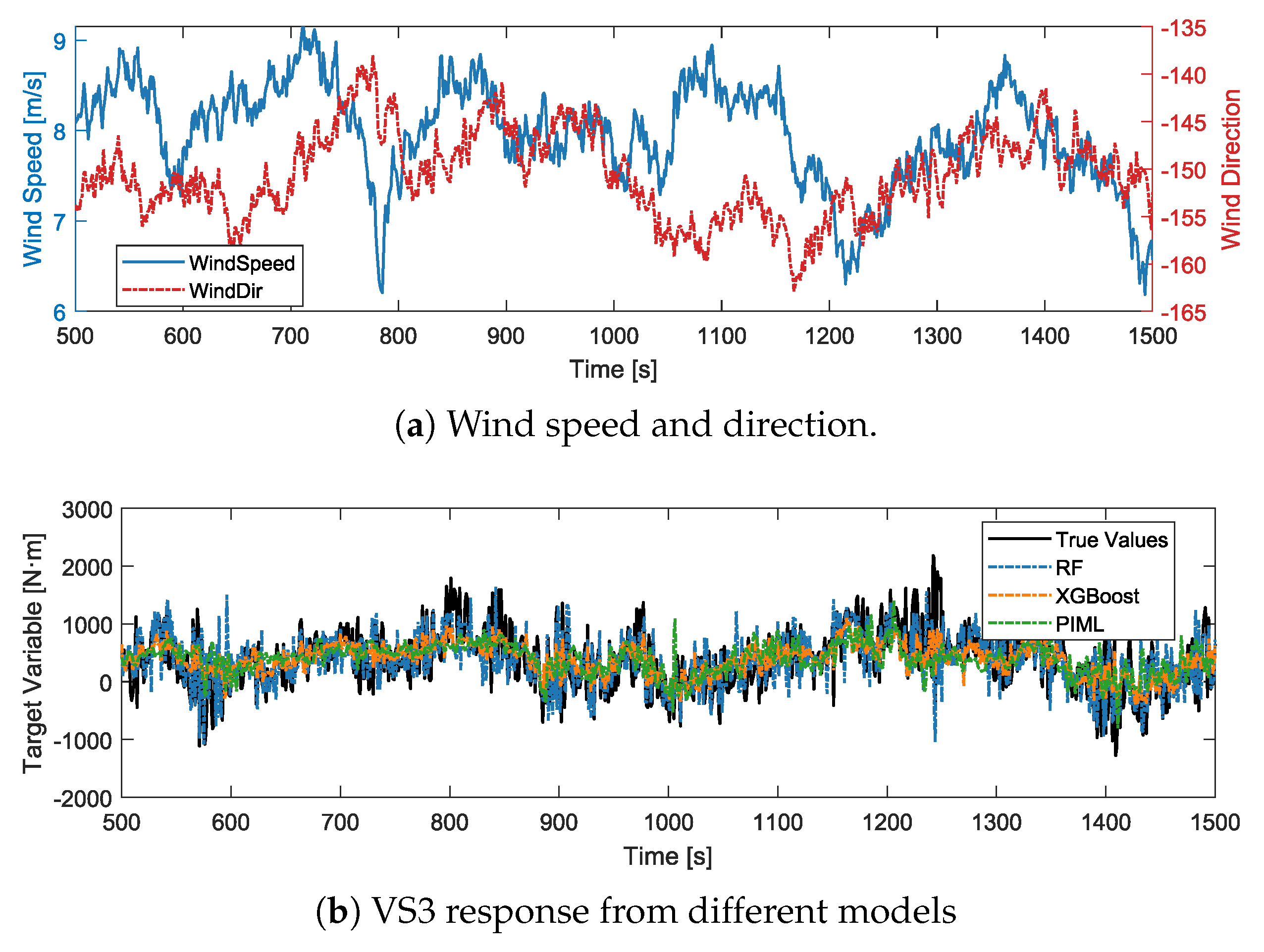
4.2. Mast Joint Bending Moment

The final subsection presents the results for the virtual sensor developed to estimate the bending moment at the top joint of the upwind mast, based solely on wind and turbine-related measurements. As in the previous case, only the XGBoost and PIML models are considered to compare purely data-driven predictions with those that incorporate physical constraints. The estimation uses wind speed, thrust, rotational speed (omega), and platform pitch as input features. The PIML model is formulated based on Equations (8) and (9). Figure 9 shows the regression results after training the virtual sensors, and Figure 10 displays the corresponding time series over a 300-s interval.

The random forest model achieved an $R^2$ score of 0.630, while XGBoost and the PIML model obtained scores of 0.791 and 0.747, respectively. Although the inclusion of basic physics-based relationships improved performance compared to the RF model, the overall accuracy remains limited. Estimating this response appears to be more difficult than in previous cases, potentially due to the absence of structural information such as vibration measurements, which are often used in related work to infer bending moments (e.g., [16]). Future studies should examine the effect of including such measurements.

5. Conclusions

This study investigated virtual sensor development for the Eolink weathervaning floating wind turbine relying on a single-point mooring system. Virtual sensors were proposed as a means to reduce reliance on physical sensors in cases where direct measurement is expected to be difficult or costly. Three virtual sensors were developed using supervised machine learning (random forest and XGBoost) and a physics-informed machine learning (PIML) approach, trained on OrcaFlex simulation data under varying conditions. The first virtual sensor estimated the force in one mooring hawser using environmental and motion inputs, demonstrating strong performance across algorithms. The second virtual sensor, estimating force in the other hawser based only on the output of the first, demonstrated improved accuracy using the PIML model compared to purely data-driven methods. The third sensor, targeting bending moments at the top joint assembly, showed lower accuracy, likely due to missing inputs related to mast accelerations or vibrations and the limitations of the simplified physics model. Overall, the results obtained using synthetic OrcaFlex data suggest that virtual sensing could be a viable approach to reduce the need for physical instrumentation in complex areas of the studied floating wind turbine, thereby providing a foundation for real-world applications.

References

1. Edwards, E.C.; Holcombe, A.; Brown, S.; Ransley, E.; Hann, M.; Greaves, D. Evolution of floating offshore wind platforms: A review of at-sea devices. Renew. Sustain. Energy Rev. 2023, 183, 113416. [Google Scholar] [CrossRef]
2. del Pozo Gonzalez, H.; Kallinger, M.D.; Rapha, J.I.; Domínguez-García, J.L. Modern Floating Wind Energy Technologies. In Energy Systems Integration for Multi-Energy Systems: From Operation to Planning in the Green Energy Context; Springer: Berlin/Heidelberg, Germany, 2025; pp. 295–316. [Google Scholar]
3. Ciuriuc, A.; Rapha, J.I.; Guanche, R.; Domínguez-García, J.L. Digital tools for floating offshore wind turbines (FOWT): A state of the art. Energy Rep. 2022, 8, 1207–1228. [Google Scholar] [CrossRef]
4. Kang, J.; Sun, L.; Soares, C.G. Fault Tree Analysis of floating offshore wind turbines. Renew. Energy 2019, 133, 1455–1467. [Google Scholar] [CrossRef]
5. Liu, Y.; Zhang, J.M.; Min, Y.T.; Yu, Y.; Lin, C.; Hu, Z.Z. A digital twin-based framework for simulation and monitoring analysis of floating wind turbine structures. Ocean Eng. 2023, 283, 115009. [Google Scholar] [CrossRef]
6. Éolink. Our Concept—Éolink. 2025. Available online: https://eolink.fr/en/our-concept/ (accessed on 26 February 2025).
7. Bernitsas, M.M.; Papoulias, F.A. Stability of single point mooring systems. Appl. Ocean Res. 1986, 8, 49–58. [Google Scholar] [CrossRef]
8. Connolly, A.; Guyot, M.; Le Boulluec, M.; Héry, L.; O’Connor, A. Fully coupled aero-hydro-structural simulation of new floating wind turbine concept. In Proceedings of the International Conference on Offshore Mechanics and Arctic Engineering, Madrid, Spain, 17–22 June 2018; American Society of Mechanical Engineers: New York, NY, USA, 2018; Volume 51975, p. V001T01A027. [Google Scholar]
9. Doisenbant, G.; Le Boulluec, M.; Scolan, Y.M.; Guyot, M. Numerical and experimental modeling of offshore wind energy capture: Application to reduced scale model testing. Wind. Eng. 2018, 42, 108–114. [Google Scholar] [CrossRef]
10. Guyot, M.; De Mourgues, C.; Le Bihan, G.; Parenthoine, P.; Templai, J.; Connolly, A.; Le Boulluec, M. Experimental offshore floating wind turbine prototype and numerical analysis during harsh and production events. In Proceedings of the International Conference on Offshore Mechanics and Arctic Engineering, Glasgow, Scotland, 9–14 June 2019; American Society of Mechanical Engineers: New York, NY, USA, 2019; Volume 59353, p. V001T02A004. [Google Scholar]
11. Guyot, M. Floating Wind Turbine Structure. U.S. Patent 9,976,540, 22 May 2018. [Google Scholar]
12. Martin, D.; Kühl, N.; Satzger, G. Virtual sensors. Bus. Inf. Syst. Eng. 2021, 63, 315–323. [Google Scholar] [CrossRef]
13. Dimitrov, N.; Göçmen, T. Virtual sensors for wind turbines with machine learning-based time series models. Wind. Energy 2022, 25, 1626–1645. [Google Scholar] [CrossRef]
14. Hlaing, N.; Morato, P.G.; Santos, F.d.N.; Weijtjens, W.; Devriendt, C.; Rigo, P. Farm-wide virtual load monitoring for offshore wind structures via Bayesian neural networks. Struct. Health Monit. 2024, 23, 1641–1663. [Google Scholar] [CrossRef]
15. Mehlan, F.C.; Keller, J.; Nejad, A.R. Virtual sensing of wind turbine hub loads and drivetrain fatigue damage. Forsch. Im Ing. 2023, 87, 207–218. [Google Scholar] [CrossRef]
16. Moynihan, B.; Tronci, E.M.; Hughes, M.C.; Moaveni, B.; Hines, E. Virtual sensing via Gaussian Process for bending moment response prediction of an offshore wind turbine using SCADA data. Renew. Energy 2024, 227, 120466. [Google Scholar] [CrossRef]
17. Gräfe, M.; Özinan, U.; Cheng, P.W. Lidar-based virtual load sensors for mooring lines using artificial neural networks. Proc. J. Phys. Conf. Ser. 2023, 2626, 012036. [Google Scholar] [CrossRef]
18. Gräfe, M.; Pettas, V.; Dimitrov, N.; Cheng, P.W. Machine-learning-based virtual load sensors for mooring lines using simulated motion and lidar measurements. Wind Energy Sci. 2024, 9, 2175–2193. [Google Scholar] [CrossRef]
19. Branlard, E.; Jonkman, J.; Brown, C.; Zhang, J. A digital twin solution for floating offshore wind turbines validated using a full-scale prototype. Wind Energy Sci. 2024, 9, 1–24. [Google Scholar] [CrossRef]
20. Pacheco-Blazquez, R.; Garcia-Espinosa, J.; Di Capua, D.; Pastor Sanchez, A. A digital twin for assessing the remaining useful life of offshore wind turbine structures. J. Mar. Sci. Eng. 2024, 12, 573. [Google Scholar] [CrossRef]
21. Walker, J.; Coraddu, A.; Collu, M.; Oneto, L. Digital twins of the mooring line tension for floating offshore wind turbines to improve monitoring, lifespan, and safety. J. Ocean Eng. Mar. Energy 2022, 8, 1–16. [Google Scholar] [CrossRef]
22. Sauder, T.; Mainçon, P.; Lone, E.; Leira, B.J. Estimation of top tensions in mooring lines by sensor fusion. Mar. Struct. 2022, 86, 103309. [Google Scholar] [CrossRef]
23. Denil, M.; Matheson, D.; De Freitas, N. Narrowing the gap: Random forests in theory and in practice. In Proceedings of the International Conference on Machine Learning, PMLR, Beijing, China, 22–24 June 2014; pp. 665–673. [Google Scholar]
24. Friedman, J.H. Stochastic gradient boosting. Comput. Stat. Data Anal. 2002, 38, 367–378. [Google Scholar] [CrossRef]
25. Patryniak, K.; Collu, M.; Coraddu, A. Rigid body dynamic response of a floating offshore wind turbine to waves: Identification of the instantaneous centre of rotation through analytical and numerical analyses. Renew. Energy 2023, 218, 119378. [Google Scholar] [CrossRef]
26. González, H.D.P.; Domínguez-García, J.L. Non-centralized hierarchical model predictive control strategy of floating offshore wind farms for fatigue load reduction. Renew. Energy 2022, 187, 248–256. [Google Scholar] [CrossRef]
27. Hall, M. Generalized Quasi-Static Mooring System Modeling with Analytic Jacobians. Energies 2024, 17, 3155. [Google Scholar] [CrossRef]
28. Mahfouz, M.Y.; Cheng, P.W. Effect of mooring system stiffness on floating offshore wind turbine loads in a passively self-adjusting floating wind farm. Renew. Energy 2025, 238, 121823. [Google Scholar] [CrossRef]
29. del Pozo Gonzalez, H.; Domínguez-García, J.L.; Gomis-Bellmunt, O. Structural motion control of waked floating offshore wind farms. Ocean Eng. 2024, 293, 116709. [Google Scholar] [CrossRef]
Figure 1. (a) Front view of the Eolink pyramidal single-point moored platform, showing the locations of the possible physical sensors. (b) Description of the moments in the pyramidal mast’s structure, and (c) top view of the angles formed by the system to align the direction of the wind force (Fwind). The zoom resumes the force in surge (Fx) and sway (Fy), while (Fm) denotes the mooring force.
Jmse 13 01411 g001
Figure 2. Workflow for virtual sensor development.
Jmse 13 01411 g002
Figure 3. Front view of the Eolink pyramidal single-point moored platform, showing the locations of the desired virtual sensors and statistics of the five most correlated variables obtained using Spearman correlation. The virtual sensor for the forces in one of the hawsers (violet upper-side box) and the statistics of the five most correlated variables related to the force in the mast fore port side, assembled at the top point (green lower-side box).
Jmse 13 01411 g003
Figure 4. A simplified scheme of the input–output of the developed virtual sensors.
Jmse 13 01411 g004
Figure 5. Regression scores of virtual sensor 1 (VS1) for force in hawser 1.
Jmse 13 01411 g005
Figure 6. Virtual sensor 1 (VS1) results for force in hawser 1. (a,b) Wind speed and direction. (c,d) Machine learning predictions compared with true values. (e,f) Hybrid model predictions compared with physics-based and true values. Left column: Hawser 1. Right column: Hawser 2.
Jmse 13 01411 g006
Figure 7. Regression scores of virtual sensor 2 (VS2) for force in hawser 2.
Jmse 13 01411 g007
Figure 8. Virtual Sensor 2 (VS2) results for the force in hawser 2. Sub-figures show: (a) regression scores using random forest; (b) regression scores using the hybrid model with best λ = 0.674 ; and (c) time series responses comparing true values (black), random forest output, and hybrid output.
Jmse 13 01411 g008
Figure 9. Regression scores of virtual sensor 3 (VS3) for top mast joint bending moment.
Jmse 13 01411 g009
Figure 10. Virtual sensor 3 (VS3) results for the top masts bending moment.
Jmse 13 01411 g010