Influence of Intense Internal Waves Traveling Along an Acoustic Path on Source Holographic Reconstruction in Shallow Water

Abstract

This paper studies how intense internal waves (IIWs) affect the holographic reconstruction of the sound field generated by a moving source in a shallow-water environment. It is assumed that the IIWs propagate along the acoustic path between the source and the receiver. The presence of IIWs introduces inhomogeneities into the waveguide and causes significant mode coupling, which perturbs the received sound field. This paper proposes the use of holographic signal processing (HSP) to eliminate perturbations in the received signal caused by mode coupling due to IIWs. Within the HSP framework, we examine the interferogram (the received sound intensity distribution in the frequency–time domain) and the hologram (the two-dimensional Fourier transform of the interferogram) of a moving source in the presence of space–time inhomogeneities caused by IIWs. A key finding is that under the influence of IIWs, the hologram is divided into two regions that correspond to the unperturbed and perturbed components of the sound field. This hologram structure enables the extraction and reconstruction of the interferogram corresponding to the unperturbed field as it would appear in a shallow-water waveguide without IIWs. Numerical simulations of HSP application under the realistic conditions of the SWARM’95 experiment were carried out for stationary and moving sources. The results demonstrate the high efficiency of holographic reconstruction of the unperturbed sound field. Unlike matched field processing (MFP), HSP does not require prior knowledge of the propagation environment. These research results advance signal processing methods in underwater acoustics by introducing efficient HSP methods for environments with spatiotemporal inhomogeneities.

1. Introduction

In recent years, there has been a growing interest among scientists in applying interferometric signal processing (ISP) techniques to the field of underwater acoustics. ISP relies on the stable characteristics of interference patterns produced by broadband acoustic fields in shallow-water waveguides [1,2]. For a comprehensive overview of ISP methodologies, readers are directed to key foundational studies such as [3,4,5]. Several studies have applied ISP to various practical tasks. For instance, in works [6,7], ISP techniques are used to estimate waveguide-invariant parameters. The study [8] demonstrates how ISP can be applied to weak signals, with signal enhancement achieved through array beamforming. In [9], ISP is used for seabed classification based on acoustic signals generated by passing vessels. A method for estimating the range to a source in shallow water using ISP is proposed in [10]. A range-independent invariant estimation approach based on ISP is explored in [11]. Furthermore, ref. [12] applies ISP to interpret interference fringes in terms of eigenray (or eigenbeam) arrival times. Finally, ISP has been adapted for deep-sea passive sonar applications in [13,14], demonstrating its versatility across different underwater acoustic environments.

One of the most promising approaches in interferometric signal processing (ISP) is known as holographic signal processing (HSP) [15,16]. The fundamental physical and mathematical principles of hologram generation were first presented in [15]. Within the HSP framework, a quasi-coherent integration of sound intensity in the frequency–time domain results in the formation of an interferogram $I(\omega ,t)$ [16]. To analyze the accumulated intensity distribution, a two-dimensional Fourier transform (2D-FT) is applied to $I(\omega ,t)$. The resulting transform is referred to as the Fourier hologram, or simply the hologram, and is denoted as $F(\tau ,\tilde{\nu })={\mathcal{F}}_{2D}\left\{I(\omega ,t)\right\}$. The hologram $F(\tau ,\tilde{\nu })$ concentrates the acoustic energy represented in $I(\omega ,t)$ into localized focal regions that arise due to the interference of different modes.

During the initial development of HSP, it was assumed that waveguide parameters remained constant in space and time. However, acoustic signal propagation in practical scenarios often occurs in waveguides affected by hydrodynamic disturbances. The application of HSP to a stationary source under real-world conditions was first explored experimentally in [17,18,19,20]. These studies demonstrated that hydrodynamic perturbations of the waveguide distort the interferogram $I(\omega ,t)$ and enlarge the focal regions in the resulting hologram $F(\tau ,\tilde{\nu })$. In the presence of inhomogeneities, the hologram $F(\tau ,\tilde{\nu })$ can be represented as a superposition of two components: one corresponding to the unperturbed waveguide and one arising from the perturbations. This two-component structure was used in [17,18,19,20] to interpret experimental data from the SWARM’95 experiment [21,22,23]. The observed waveguide inhomogeneities during the SWARM’95 experiment were primarily caused by intense internal waves (IIWs) [21,22,23], a widespread hydrodynamic phenomenon in the ocean [24,25,26]. In the SWARM’95 experiment, two acoustic paths were used, which were formed by a single source and two spatially separated vertical receiving arrays. The first acoustic path was oriented at a small angle to the wavefront of IIWs. The presence of IIW structures induces a pronounced horizontal refraction of the acoustic rays. In our previous paper [27], we analyzed the variations in the hologram structure of a moving source in cases of significant horizontal refraction of sound rays due to IIWs. In the SWARM’95 experiment, the second acoustic path was oriented across the wavefront of the IIWs. With this orientation, the IIWs propagated along the acoustic path between the source and receiver. In this case, the IIWs did not cause horizontal refraction but rather led to significant scattering of sound energy between acoustic modes. In other words, they induced mode coupling. This phenomenon was not considered in our previous paper [27]. However, understanding the features of hologram structure variations caused by significant mode coupling due to IIWs is crucial for developing HSP. Therefore, the current paper is dedicated to analyzing this phenomenon.

This paper aims to study the influence of intense internal waves (IIWs) on the holographic reconstruction of a moving source sound field in shallow water in the presence of IIWs traveling along the acoustic path between the source and the receiver, which cause significant coupling between acoustic modes. This study is based on numerical simulations that consider mode coupling induced by internal wave activity. Within this framework, we examine the interferogram (the received sound intensity distribution in the frequency–time domain) and the hologram (2D-FT of the interferogram) of moving sources in the presence of space–time inhomogeneities caused by intense internal waves. One of the paper’s key findings is that under the influence of internal waves, the hologram is divided into two distinct regions corresponding to the unperturbed and perturbed components of the sound field, respectively. This structure allows us to extract and reconstruct the interferogram corresponding to the unperturbed field as it would appear in a shallow-water waveguide without internal waves. The paper also provides an estimate of the error associated with holographic reconstruction using HSP.

Our research relies on numerical simulations of sound field propagation in three-dimensional (3D) inhomogeneous shallow-water waveguides. The structure of the sound field can be significantly affected by 3D inhomogeneities in the propagation medium due to sound scattering by IIWs. Modeling broadband, low-frequency sound fields in these 3D environments requires significant computational resources and often necessitates advanced numerical methods and high-performance computing platforms to ensure physically realistic results. There are five principal groups of numerical approaches for simulating sound field propagation in inhomogeneous shallow-water waveguides [28]: 3D Helmholtz equation (3DHE) models [29,30,31]; 3D parabolic equation (3DPE) models [32,33,34,35,36,37,38]; 3D ray-based (3DR) models [39,40,41]; vertical modes and 2D modal parabolic equation (VMMPE) models [27,42,43,44,45]; and vertical coupled modes with horizontal rays (VCMHR) models [46,47,48,49,50,51,52,53,54,55,56,57,58,59].

Our research focuses on the low-frequency sound field within two frequency bands: 100–120 Hz and 300–320 Hz. We assume that the spatial inhomogeneities of the shallow-water waveguide are generated by IIW inhomogeneities propagating along the acoustic path between the source and the receiver. These inhomogeneities, induced by IIWs, lead to strong scattering effects. Of the five modeling approaches mentioned, the VCMHR model is the most suitable for our scenario. It is well-adapted to low-frequency sound propagation in a shallow-water waveguide with IIWs. The VCMHR model accurately incorporates boundary conditions and captures the essential physics of vertical mode coupling due to environmental variability. In contrast, 3D models are generally better suited to high-frequency scenarios and fail to adequately describe mode coupling at low frequencies in shallow water. Although the 3DHE and 3DPE methods provide high-fidelity solutions, they are computationally prohibitive in this context due to the complexity of the 3D problem. VMMPE models, on the other hand, effectively handle horizontal refraction but lack sufficient capability for mode coupling, a key process in our paper. Therefore, we selected the VCMHR framework as the most appropriate numerical tool for simulating sound field propagation under the influence of IIWs.

In our study, we model the shallow-water waveguide with spatial and temporal variability induced by IIWs. A central assumption of the simulation is that the speed of acoustic wave propagation (∼1500 m/s) is considerably higher than the motion speed of the source (∼0.5–5 m/s) and the propagation speed of IIWs (∼0.5–1 m/s). We apply the “frozen environment” approximation [41,60], which posits that the acoustic medium remains effectively static while the signal propagates from the source to the receiver.

The holographic processing approach developed in our work is an effective alternative to the well-established matched field processing (MFP) technique [61,62,63,64,65]. Although MFP is widely used in underwater acoustics, its practical application is limited by several critical constraints. Specifically, MFP methods require highly detailed and accurate knowledge of the propagation environment, including a precise characterization of the water column and the properties of the sea bottom [61,62]. However, these requirements often prove difficult to satisfy in real-world scenarios, particularly in shallow-water waveguides. The method’s performance is notably vulnerable to model mismatch due to incomplete or inaccurate environmental data. These issues are especially pronounced in shallow-water environments where reliable bathymetric and geoacoustic information is typically scarce or absent. Dynamic processes such as internal waves, tides, and stratification variability introduce significant temporal fluctuations in the sound–speed profile. Consequently, the effectiveness of conventional MFP can be severely compromised in such complex, time-varying conditions [63,64]. In contrast, the proposed holographic method is more robust in the face of environmental uncertainty and can operate effectively. It can even operate in the absence of prior knowledge about the waveguide, offering a promising solution for real-time, adaptive acoustic sensing applications in challenging marine environments [65].

The numerical implementation of the simulation used in our study has been validated multiple times against various experimental datasets, including SWARM’95, ASIAEX’01, and SHALLOW WATER’06. In particular, we validated our numerical implementation while processing and analyzing experimental data obtained from the SWARM’95 experiment [23]. Additionally, the HSP developed in the paper was verified using SWARM’95 data [17,18,19,20]. Studies based on SWARM’95 data demonstrate that the source-generated hologram splits into two components in the presence of IIWs: one corresponds to the waveguide without internal waves; the other results from perturbations caused by IIW activity [17,18,19,20]. Unfortunately, it was not possible to assess the accuracy of source interferogram reconstruction in the absence of IIW during the experiment, as such data were unavailable. Therefore, the research presented in this paper is a significant step forward in developing the HSP approach. The numerical simulations conducted in this study enable a comparative analysis of the original and reconstructed source interferograms.

This paper is organized into six sections. After the introduction in Section 1, Section 2 describes the 3D model of a shallow-water waveguide in the presence of IIWs traveling along an acoustic path. Next, in Section 3, we derive the mathematical model of the interferogram $I(\omega ,t)$ and, in Section 4, the hologram $F(\tau ,\tilde{\nu })$ of a moving source in a shallow-water waveguide with significant mode coupling caused by IIWs. We develop an algorithm for the numerical calculation of the interferogram and hologram of a moving source. It is based on a set of differential equations for the mode amplitudes. This algorithm takes into account the mode coupling caused by IIWs propagating along the acoustic path between the source and receiver. In Section 5, we analyze the results of the numerical modeling of the interferogram $I(\omega ,t)$ and hologram $F(\tau ,\tilde{\nu })$ of a broadband sound source in a shallow-water waveguide in the presence of IIWs causing significant mode coupling. The numerical modeling considers the influence of IIWs on the interferogram $I(\omega ,t)$ and hologram $F(\tau ,\tilde{\nu })$ of the source sound field for two cases of source parameters. The first case involves a stationary acoustic path between the source and the receiver (non-moving source). The second case involves a non-stationary acoustic path (i.e., a moving source). To compare the numerical modeling results for both cases in the presence of IIWs, the initial data for the simulations are chosen to be the same. The influence of IIWs on holographic reconstruction error is analyzed. The results are summarized in Section 6 of this paper.

2. Waveguide Model in the Presence of IIWs

The waveguide model in IIWs propagating along the acoustic path is presented in Section 2, which consists of two parts. The first part, Section 2.1, describes the shallow-water waveguide model with inhomogeneities due to IIWs. Section 2.2 examines the model of IIWs and its parameters.

2.1. Waveguide Model with Inhomogeneities Due to IIWs

In this section, we present the three-dimensional model of the shallow-water waveguide used in our study (see Figure 1). The waveguide is defined in a Cartesian coordinate system $(X,Y,Z)$ and modeled as a water layer with spatially and temporally varying sound speed $c(\mathbf{r},z,t)$ and density $\rho (\mathbf{r},z,t)$. Here, $\mathbf{r}=(x,y)$ denotes the horizontal position vector. The water column is bounded above by the free surface at $z=0$ and below by the sea bottom at $z=H$.

The density and refractive index of the seabed are given by ${\rho }_b$ and $n_b(1+\mathrm{i}\varkappa )$, respectively [41,60], where $\varkappa$ is the attenuation factor, defined as $\varkappa =\chi c_b/\left(54.6f\right)$. In this expression, $\chi$ represents the bottom loss coefficient, $c_b$ is the acoustic velocity in the bottom layer, and f is the sound frequency.

The spatiotemporal variation of the sound speed within the water column can be expressed as

$$c(\mathbf{r},z,t)=\overline{c}\left(z\right)+\tilde{c}(\mathbf{r},z,t),$$

(1)

where $\overline{c}\left(z\right)$ is the background sound speed profile in the absence of internal wave activity, and $\tilde{c}(\mathbf{r},z,t)$ accounts for the perturbations induced by internal inertia waves (IIWs).

Based on Equation (1), the squared refractive index in the water column is given by

$$n^2(\mathbf{r},z,t)={\overline{n}}^2\left(z\right)+{\tilde{n}}^2(\mathbf{r},z,t),$$

(2)

where ${\overline{n}}^2\left(z\right)$ is the unperturbed refractive index profile, and ${\tilde{n}}^2(\mathbf{r},z,t)$ is the fluctuation component caused by IIWs. Following the formulation in [26,43], the perturbation term can be described as

$${\tilde{n}}^2(\mathbf{r},z,t)=-2Q{N}^2\left(z\right)\zeta (\mathbf{r},z,t),$$

(3)

where $Q\approx 2.4{\mathrm{s}}^2/\mathrm{m}$ is a water-specific physical constant, $N\left(z\right)={\left(-{\displaystyle \frac{g}{\rho }}{\displaystyle \frac{d\rho }{dz}}\right)}^{1/2}$ is the buoyancy frequency, and $\zeta (\mathbf{r},z,t)$ denotes the vertical displacements within the water column induced by IIWs.

2.2. IIWs Parameters

In this section, we present a space–time model of IIWs $\zeta (\mathbf{r},z,t)$ and their parameters. According to the predominance of the first gravity mode [24,25,26], vertical displacements within the water column induced by IIWs can be expressed as follows:

$$\zeta (\mathbf{r},z,t)={\Phi }_1\left(z\right){\zeta }_0(\mathbf{r},t),$$

(4)

where ${\Phi }_1\left(z\right)$ denotes the eigenfunction of the first gravity mode, normalized at depth $z_0$: ${\Phi }_1\left(z_0\right)=1$. According to [24,25,26], the gravity modes ${\Phi }_n\left(z\right)$ and their corresponding dispersion characteristics ${\Omega }_n\left(K\right)$ represent the eigenfunctions and eigenvalues of the following Sturm–Liouville problem:

$${\displaystyle \frac{d^2{\Phi }_n\left(z\right)}{d{z}^2}}+\left({\displaystyle \frac{N^2\left(z\right)}{{\Omega }_n^2\left(K\right)}}-1\right)K^2{\Phi }_n\left(z\right)=0,{\Phi }_n\left(0\right)={\Phi }_n\left(H\right)=0.$$

(5)

The gravity modes ${\Phi }_n\left(z\right)$ satisfy the following normalization condition [24,25,26]:

$${\int }_0^H{N}^2\left(z\right){\Phi }_n\left(z\right){\Phi }_m\left(z\right)dz={\delta }_{nm},$$

(6)

where ${\delta }_{nm}$ is the Kronecker delta. For typical stratifications on the continental shelf, the function $\Phi \left(z\right)$ depends weakly on the frequency and the wave number. In Equation (4), $\zeta (\mathbf{r},z,t)={\zeta }_0(x,y,t)$ are the vertical displacements in the waveguide water layer due to IIWs at a depth $z_0$ in the thermocline water layer.

According to [24,25,26], we can represent IIWs as a sequence of internal solitons (IS), which are soliton-like solutions of the Korteweg–de Vries (KdV) equation:

$${\displaystyle \frac{\partial {\zeta }_0}{\partial t}}+u{\displaystyle \frac{\partial {\zeta }_0}{\partial x}}+a{\zeta }_0{\displaystyle \frac{\partial {\zeta }_0}{\partial x}}+b{\displaystyle \frac{{\partial }^3{\zeta }_0}{\partial x^3}}=0.$$

(7)

The parameters of Equation (7) are determined by the stratification of the water layer:

$$a={\displaystyle \frac{3u}{2}}{\int }_0^H{\left({\displaystyle \frac{d\Phi }{dz}}\right)}^{3}dz/{\int }_0^H{\left({\displaystyle \frac{d\Phi }{dz}}\right)}^{2}dz,$$

(8)

$$b={\displaystyle \frac{u}{2}}{\int }_0^H{\Phi }^{2}dz/{\int }_0^H{\left({\displaystyle \frac{d\Phi }{dz}}\right)}^{2}dz,u={\displaystyle \frac{\Omega \left(K\right)}{K}}$$

(9)

Given the selected geometry of the problem (see Figure 2), the vertical displacement ${\zeta }_0(\mathbf{r},t)$ in the water layer of the waveguide can be represented as follows:

$${\zeta }_0(\mathbf{r},t)=\sum _{n=1}^N{B}_n{sech}^2\left[{\displaystyle \frac{x-D_n-u_{n}t}{{\eta }_n}}\right],$$

(10)

where N denotes the number of internal solitons (IS) in the train, $B_n$ is the amplitude of the n-th soliton, $u_n$ is the propagation speed, $D_n$ is the initial horizontal displacement, and ${\eta }_n$ is the width of the soliton.

IIWs are a widespread phenomenon in the ocean. They are trains of short-period vertical displacements of water layers. They are described as trains of IS that propagate to the shelf coast. IIWs are caused by internal tides [24,25,26]. The parameters of IIWs are presented in

Table 1. Parameters of IIWs.

Parameter	Value
Train length	$L\sim 3$–5 km
Count of internal solitons	$N\sim 4$–7
Traveling velocity	$u_n\sim 0.5$–1 m/s
Internal soliton amplitude	$B_n\sim 10$–30 m
Internal soliton width	${\eta }_n\sim 100$–200 m
Interval between solitons	$D_n\sim 300$–500 m
Curvature radius of wave front	$R\sim 15$–25 km

in accordance with the experimental data [21,22,24,25,26]. These parameters lead to specific acoustic phenomena due to IIWs. The study in [43] demonstrates that IIWs traveling across the acoustic path between the source and receiver significantly influence the horizontal refraction of acoustic rays propagating at small angles relative to the IIW wavefronts. Consequently, the resulting dynamic waveguides in the horizontal plane align nearly parallel to the IIW fronts. The impact of this acoustic phenomenon on the holographic structure generated by a moving source was examined in detail in our previous paper [60]. Conversely, IIWs propagating along the acoustic path between the source and receiver induce strong coupling between acoustic modes. This mode coupling results in a redistribution of sound energy across the modes, altering the balance of modal amplitudes within the sound field structure. The following sections of the paper analyze how these effects influence the process of source holographic reconstruction.

The “vertical modes and horizontal rays” approach shows that horizontal dynamic waveguides are selective for sound modes. The structure of horizontal rays differs for different sound modes. The structure of the horizontal rays of the sound modes also depends on frequency, as shown in [43]. The resonance-like form of this frequency dependence is evident in the propagation of broadband sound signals.

3. Structure of the Source Interferogram Due to IIWs

This section presents the model of the source interferogram in the presence of IIWs propagating along the acoustic path. It consists of three parts. The first part (Section 3.1) describes the sound field model in a waveguide with IIWs, using the vertical modes and horizontal rays approximation framework. Section 3.2 presents the mode coupling approach to account for the sound field due to inhomogeneities caused by IIWs. Section 3.3 considers the structure of the interferogram of a broadband source moving in a waveguide in the presence of IIWs.

3.1. Sound Field Model in a Waveguide with IIWs

Within the framework of the vertical modes and horizontal rays approximation, the complex acoustic field in a shallow waveguide influenced by IIWs, which is described by Equations (1)–(10), can be expressed as follows, cf. [41,42,43,60]:

$$p(\mathbf{r},z,\omega ,t)=\sum _{m=0}^M{P}_m(\mathbf{r},\omega ,t){\varphi }_m(z,\omega ),$$

(11)

Here, $\mathbf{r}=(x,y)$ denotes the horizontal position vector of the source, $P_m$ represents the amplitude of the m-th mode, and ${\varphi }_m(z,\omega )$ denotes the vertical structure (mode shape) of the corresponding acoustic mode in a waveguide unaffected by IIWs. The complex horizontal wavenumber of each mode is given by ${\overline{\xi }}_m\left(\omega \right)={\overline{h}}_m(\mathbf{r},\omega ,t)+\mathrm{i}{\overline{\gamma }}_m(\mathbf{r},\omega ,t)$, where ${\overline{h}}_m$ and ${\overline{\gamma }}_m$ are its real and imaginary parts, respectively. The summation extends to M, the total number of modes considered. As a result, the acoustic pressure field p depends on the angular frequency $\omega =2\pi f$. The eigenfunctions ${\varphi }_m(z,\omega )$ and the complex wavenumbers ${\overline{\xi }}_m$ are obtained by solving the associated Sturm–Liouville eigenvalue problem with boundary conditions corresponding to a free surface and a bottom, cf. [41,60]:

$${\displaystyle \frac{d^2{\varphi }_m(\omega ,z)}{d{z}^2}}+k^2{\overline{n}}^2\left(z\right){\varphi }_m(\omega ,z)={\overline{\xi }}_m^2{\varphi }_m(\omega ,z),$$

(12)

$${\varphi }_m(\omega ,z){|}_{z=0}=0,{\varphi }_m(\omega ,z){|}_{z=H}+g\left({\overline{\xi }}_m\right){\displaystyle \frac{d{\varphi }_m(\omega ,z)}{dz}}{|}_{z=H}=0,$$

(13)

where

$$g\left({\xi }_m\right)=\eta /\sqrt{{\overline{\xi }}_m^2-k^2{n}_b^2(1+\mathrm{i}\varkappa )}.$$

(14)

The functions ${\varphi }_m(\omega ,z)$ are orthonormalized:

$${\int }_0^H{\varphi }_l{\varphi }_{m}dz+\eta {\int }_H^{\infty }{\varphi }_l{\varphi }_{m}dz={\delta }_{ml},$$

(15)

where ${\delta }_{ml}$ is the Kronecker delta symbol.

3.2. Coupling Modes Due to IIWs

Let us consider the coupled-mode approach [41,46,47,48,49,50,51] to take into account the scattering of the sound field Equation (11) induced by the inhomogeneities of the water layer caused by IIWs. In the mode amplitude $P_m(\mathbf{r},\omega ,t)$, we isolate the factor corresponding to cylindrical spreading:

$$P_m(\mathbf{r},\omega ,t)={\displaystyle \frac{C_m(\mathbf{r},\omega ,t)}{\sqrt{{\overline{h}}_{m}r}}},$$

(16)

where $C_m(\mathbf{r},\omega ,t)$ denotes the mode amplitude without the cylindrical spreading factor, and ${\overline{h}}_m$ is the real part of the mode horizontal wavenumber. The horizontal range between the source and the receiver is r. This representation explicitly factors out the geometric spreading term $1/\sqrt{r}$, which dominates the range dependence in the shallow-water waveguide under consideration.

Under the forward-scattering approximation, the Helmholtz equation for the sound field reduces to a first-order system of ordinary differential equations that describes the evolution of coupled mode amplitudes $C_m(r,\omega ,t)$:

$${\displaystyle \frac{d{C}_m(r,\omega ,t)}{dr}}=\mathrm{i}\sum _{l=1}^M\left({\overline{\xi }}_m{\delta }_{ml}+{\mu }_{ml}(r,\omega ,t)\right)C_l(r,\omega ,t).$$

(17)

Here, the complex mode horizontal wavenumber is defined as ${\overline{\xi }}_m\left(\omega \right)={\overline{h}}_m(\mathbf{r},\omega ,t)+\mathrm{i}{\overline{\gamma }}_m(\mathbf{r},\omega ,t)$. The mode coupling coefficients due to IIWs are ${\mu }_{ml}(r,\omega ,t)$:

$${\mu }_{ml}(r,\omega ,t)={\displaystyle \frac{k^2}{2\sqrt{{\overline{h}}_m{\overline{h}}_l}}}{\int }_0^H{\varphi }_m(\omega ,z){\tilde{n}}^2(\mathbf{r},z,t),{\varphi }_l(\omega ,z)dz.$$

(18)

Thus, the problem of simulating the sound field in an inhomogeneous, shallow-water waveguide with IIWs can be reduced to determining the waveguide modes without IIWs (see Equations (12)–(15)) and solving the system of differential equations for the coupling mode amplitudes (see Equations (17) and (18)). This system of differential equations must be supplemented with an initial source condition. For a point omnidirectional source located at the coordinates $r=r_0$ and $z=z_0$, this condition takes the form $C_m(0,\omega ,t)={\varphi }_m(\omega ,z_0)$, up to a constant factor.

The numerical solution of Equations (17) and (18) has the following matrix form:

$$\mathbf{C}(r+\Delta r,\omega ,t)=exp\left\{\mathrm{i}\mathbf{M}(r,\omega ,t)\Delta r\right\}\mathbf{C}(r,\omega ,t).$$

(19)

Here, $\mathbf{C}(r,\omega ,t)=\left\{C_m(r,\omega ,t)\right\}$ is the vector of the mode amplitudes; $\mathbf{C}\left(0\right)=\left\{C_m(0,\omega ,t)\right\}$ is the vector of initial amplitude values. The matrix of mode coupling coefficients $\mathbf{M}(r,\omega ,t)$ has the following form:

$$\mathbf{M}(r,\omega ,t)=\left\{{\overline{\xi }}_m(r,\omega ){\delta }_{nm}+{\mu }_{nm}(r,\omega ,t)\right\}.$$

(20)

3.3. Interferogram Structure of a Moving Source in the Presence of IIWs

In the “vertical modes and horizontal rays approximation” framework, Equation (11), the interferogram $I(\omega ,t)$ of the moving source in the frequency–time domain $(\omega ,t)$ can be written as:

$$\begin{array}{cc}\hfill I(\omega ,t)& =\sum _m\sum _n{A}_m(\omega ,t)A_n^{*}(\omega ,t)exp\left[\mathrm{i}{\overline{h}}_{mn}\left(\omega \right)(x_0-vt)\right]\hfill \\ \hfill & =\sum _m\sum _n{I}_{mn}(\omega ,t),m\ne n,\hfill \end{array}$$

(21)

where ${\overline{h}}_{mn}\left(\omega \right)={\overline{h}}_m\left(\omega \right)-{\overline{h}}_n\left(\omega \right)$. Here, $I_{mn}(\omega ,t)$ is the partial interferogram due to interference of m-th and n-th modes, $A_m(\omega ,t)$ is the amplitude of the $m$-th acoustic mode ($A_m(\omega ,t)=P_m(\omega ,t){\varphi }_m(z,\omega )exp(-\mathrm{i}{\overline{h}}_{m}r)$), $x_0$ is the initial source coordinate at time $t_0=0$, t is the current time, and v is the velocity of the moving source. The superscript “*” denotes the complex conjugate value. The condition $m\ne n$ means that the mean value has been removed from the interferogram $I(\omega ,t)$.

4. Structure of the Source Hologram Due to IIWs

In this section, we examine the holographic representation of a moving acoustic source in the presence of IIWs interactions. To extract holographic features, we apply a 2D-FT to the interferogram $I(\omega ,t)$ from Equation (21) in the joint frequency–time domain $(\omega ,t)$. This yields the hologram $F(\tau ,\tilde{\nu })$ in the following form:

$$\begin{array}{cc}\hfill F(\tau ,\tilde{\nu })& =\sum _m\sum _n{\int }_0^{\Delta t}{\int }_{{\omega }_1}^{{\omega }_2}{I}_{mn}(\omega ,t)exp\left[\mathrm{i}(\tilde{\nu }t-\omega \tau )\right]dtd\omega \hfill \\ \hfill & =\sum _m\sum _n{F}_{mn}(\tau ,\tilde{\nu }),\hfill \end{array}$$

(22)

where $\tau$ is the time lag and $\tilde{\nu }=2\pi \nu$ is the angular frequency in the hologram domain. The quantity $F_{mn}(\tau ,\tilde{\nu })$ corresponds to the modal interference between the m-th and n-th acoustic modes. The frequency integration is performed over the range ${\omega }_1={\omega }_0-\Delta \omega /2$ to ${\omega }_2={\omega }_0+\Delta \omega /2$. Here, $\Delta \omega$ is the bandwidth of the signal, ${\omega }_0$ is the central (reference) frequency, and $\Delta t$ is the duration of the observation. To further simplify the analysis, we use a linearized approximation of modal dispersion:

$${\overline{h}}_m\left(\omega \right)={\overline{h}}_m\left({\omega }_0\right)+{\displaystyle \frac{d{\overline{h}}_m}{d\omega }}{|}_{\omega ={\omega }_0}(\omega -{\omega }_0).$$

(23)

Assuming that the frequency dependence of the modal amplitudes, $P_m$, and the spectral content of the sound field vary slowly compared to the rapid phase oscillations of the term $exp\left[\mathrm{i}{h}_m\left(\omega \right)(x_0+vt)\right]$, the expression for the partial hologram in Equation (22) can be rewritten in a simplified form:

$$\begin{array}{cc}{F}_{mn}(\tau ,\tilde{\nu })=\hfill & A_m\left({\omega }_0\right)A_n^{*}\left({\omega }_0\right)\Delta \omega \Delta texp\left[\mathrm{i}{\Phi }_{mn}(\tau ,\tilde{\nu })\right]\hfill \\ & \hfill \times {\displaystyle \frac{sin\left\{\left[x_0{\displaystyle \frac{\mathrm{d}{\overline{h}}_{mn}\left({\omega }_0\right)}{\mathrm{d}\omega }}-\tau \right]{\displaystyle \frac{\Delta \omega }{2}}\right\}sin\left\{\left[v{\overline{h}}_{mn}\left({\omega }_0\right)+\tilde{\nu }\right]{\displaystyle \frac{\Delta t}{2}}\right\}}{\left[x_0{\displaystyle \frac{\mathrm{d}{\overline{h}}_{mn}\left({\omega }_0\right)}{\mathrm{d}\omega }}-\tau \right]{\displaystyle \frac{\Delta \omega }{2}}\left[v{\overline{h}}_{mn}\left({\omega }_0\right)+\tilde{\nu }\right]{\displaystyle \frac{\Delta t}{2}}}},\end{array}$$

(24)

where ${\Phi }_{mn}(\tau ,\tilde{\nu })$ is the phase of the $F_{mn}(\tau ,\tilde{\nu })$—partial hologram

$${\Phi }_{mn}(\tau ,\tilde{\nu })=\left({\displaystyle \frac{\tilde{\nu }\Delta t}{2}}-\tau {\omega }_0\right)+{\overline{h}}_{mn}\left({\omega }_0\right)\left({\displaystyle \frac{\Delta t}{2}}v+x_0\right).$$

(25)

It is important to note that Equation (24) is derived under the assumption that $x_0\gg v\Delta t$. In the $(\tau ,\tilde{\nu })$ domain, the hologram $F(\tau ,\tilde{\nu })$ is concentrated within two compact regions that appear as focal spots. These regions are positioned as follows:

• The I and III quadrants if the source moves toward the receiver ($v<0$);
• The II and IV quadrants if the source moves away from the receiver ($v>0$).

The distribution $F(\tau ,\tilde{\nu })$ contains $M-1$ distinct focal spots, each of which is located at the coordinates $({\tau }_{\mu },{\tilde{\nu }}_{\mu })$ along a straight line defined by the equation $\tilde{\nu }=\tilde{\epsilon }\tau$. The index $\mu =1,2,\dots ,M-1$ enumerates the focal spots. Each spot at $({\tau }_{\mu },{\tilde{\nu }}_{\mu })$ represents a location where the maxima of $M-\mu$ partial holograms constructively interfere. The slope $\tilde{\epsilon }=2\pi \epsilon$ of this line can also be expressed as $\tilde{\epsilon }=-\delta \omega /\delta t$. Here, $\delta \omega$ is the shift in frequency corresponding to the peak of the interference pattern over the time interval $\delta t$.

The dimensions of each focal spot along the $\tau$ and $\tilde{\nu }$ axes are identical for all spots and independent of their total count. These dimensions are given by:

$$\delta \tau ={\displaystyle \frac{4\pi }{\delta \omega }},\delta \tilde{\nu }={\displaystyle \frac{4\pi }{\delta t}}.$$

(26)

The initial distance and radial velocity of the source can be determined for the focal spot nearest to the origin of the hologram plane using the following expressions from [16]:

$$\dot{v}=-k_v{\tilde{\nu }}_1,{\dot{x}}_0=k_x{\tau }_1,$$

(27)

where

$$k_v=(M-1){\left(h_{1M}\left({\omega }_0\right)\right)}^{-1},k_x=(M-1){\left(\mathrm{d}{h}_{1M}\left({\omega }_0\right)/\mathrm{d}\omega \right)}^{-1}.$$

(28)

Unlike the actual source parameters, the values estimated through processing are denoted with an overdot. The holographic signal processing technique is implemented as follows. During the total observation window $\Delta t$, the interferogram $I(\omega ,t)$ is constructed by quasi-coherently summing J statistically independent realizations of the received signal. Each realization has a duration of $t_1$ and is separated from the others by a time gap of $t_2$. This is performed over the frequency range of $\Delta \omega$. The number of realizations is given by:

$$J={\displaystyle \frac{\Delta t}{t_1+t_2}}.$$

(29)

To ensure statistical independence between realizations, the condition $t_2>2\pi /\Delta \omega$ must be satisfied. Then, the constructed interferogram $I(\omega ,t)$ is transformed using 2D-FT, resulting in the hologram $F(\tau ,\tilde{\nu })$ corresponding to the moving source in the waveguide environment.

In general, the spatial–spectral structure of the hologram $F(\tau ,\tilde{\nu })$ differs significantly from that of the original interferogram $I(\omega ,t)$. Nevertheless, a one-to-one correspondence exists between them: the hologram $F(\tau ,\tilde{\nu })$ uniquely represents the content of the interferogram $I(\omega ,t)$. Thus, applying an inverse 2D-FT to $F(\tau ,\tilde{\nu })$ allows for the complete reconstruction of the initial interferogram $I(\omega ,t)$.

5. Numerical Simulation Results

This section discusses the outcomes of numerical simulations concerning the interferogram $I(\omega ,t)$ and the hologram $F(\tau ,\tilde{\nu })$ for a broadband acoustic source in a shallow-water waveguide. The simulations account for intense internal waves (IIWs), which induce mode coupling. The simulation examines the effects of IIWs on the interferogram and hologram of the source’s acoustic field under two different source configurations. The first scenario uses a fixed source–receiver geometry (i.e., a stationary source), and the second uses a dynamic configuration with a moving source. To enable meaningful comparisons of the effects of IIWs in both scenarios, the simulations use identical initial parameters.

Section 5 is divided into three subsections. Section 5.1 details the characteristics of the shallow-water waveguide and the parameters of the acoustic source. Section 5.2 presents the modeling results for the stationary source case. Section 5.3 provides an analysis of the results for the moving source configuration.

5.1. Shallow-Water Waveguide and Sound Field Parameters

The waveguide model used in the simulation is based on parameters representative of the SWARM’95 experiment, conducted off the coast of New Jersey in 1995 [21,22]. In the numerical calculations, the sound speed profile $c\left(z\right)$ is adopted according to observational data collected in the experimental area between 18:00 and 20:00 GMT on 4 August 1995 [21].

Numerical modeling is carried out for the acoustic parameters of a shallow-water waveguide (see

Table 2. Acoustic parameters of shallow-water waveguide.

Parameter	$\mathbf{\Delta }{\mathit{f}}_1=100$–120 Hz	$\mathbf{\Delta }{\mathit{f}}_2=300$–320 Hz
Bottom refractive index	$n_b=0.84(1+\mathrm{i}0.03)$	$n_b=0.84(1+\mathrm{i}0.05)$
Bottom density	${\rho }_b=1.8$ g/cm3	${\rho }_b=1.8$ g/cm3
Mode count	$M=4$	$M=10$

). Two frequency bands are considered: $\Delta f_1=100$–120 Hz and $\Delta f_2=300$–320 Hz. For the first frequency band $\Delta f_1$, the bottom refractive index is $n_b=0.84(1+\mathrm{i}0.03)$, the bottom density is ${\rho }_b=1.8$ g/cm³, and the mode count is $M=4$. For the second frequency band $\Delta f_2$, the bottom refractive index is $n_b=0.84(1+\mathrm{i}0.05)$, the bottom density is ${\rho }_b=1.8$ g/cm³, and the mode count is $M=10$. The initial range is $x_0=10$ km between the source and the receiver. The depth of the source is $z_s=12.5$ m. The depth of the receiver is $z_q=35$ m. The source spectrum is uniform. Sound pulses are recorded periodically at an interval of 5 s. The sampling frequency is $0.25$ Hz. The observation time is $T=20$ min.

In the first frequency band $\Delta f_1=100$–120 Hz, the sound field consists of $M=4$ propagating modes. The parameters of the sound field mode, $h_m\left({\omega }_0\right)$ and their frequency derivatives ${\displaystyle \frac{d{h}_m\left({\omega }_0\right)}{d\omega }}$, are presented in

Table 3. Sound field mode parameters ($\Delta f_1=100$–120 Hz).

m-th Mode	${\mathit{h}}_{\mathit{m}}$, m−1	$({\mathit{dh}}_{\mathit{m}}/\mathit{d}\mathit{\omega })\times {10}^4$, (m/s)−1
1	0.4635	6.762
2	0.4557	6.808
3	0.4450	6.901
4	0.4310	7.091

. As can be seen, $h_m\left({\omega }_0\right)\sim 0.43$–$0.46$ m⁻¹ and ${\displaystyle \frac{d{h}_m\left({\omega }_0\right)}{d\omega }}\sim 6.7·{10}^4$–$7.1·{10}^4$ (m/s)⁻¹.

In the second frequency band, $\Delta f_2=300$–320 Hz, the sound field consists of $M=10$ propagating modes. The parameters of the sound field mode, $h_m\left({\omega }_0\right)$ and their frequency derivatives ${\displaystyle \frac{d{h}_m\left({\omega }_0\right)}{d\omega }}$, are presented in

Table 4. Sound field mode parameters ($\Delta f_2=300$–320 Hz).

m-th Mode	${\mathit{h}}_{\mathit{m}}$, m−1	$({\mathit{dh}}_{\mathit{m}}/\mathit{d}\mathit{\omega })\times {10}^4$, (m/s)−1
1	1.312	6.751
2	1.307	6.761
3	1.300	6.781
4	1.292	6.797
5	1.282	6.808
6	1.273	6.815
7	1.263	6.831
8	1.252	6.875
9	1.240	6.970
10	1.225	7.057

. As can be seen in Table 4, $h_m\left({\omega }_0\right)\sim 1.2$–$1.3$ m⁻¹ and ${\displaystyle \frac{d{h}_m\left({\omega }_0\right)}{d\omega }}\sim 6.7\times {10}^4$–$7.1\times {10}^4$ (m/s)⁻¹.

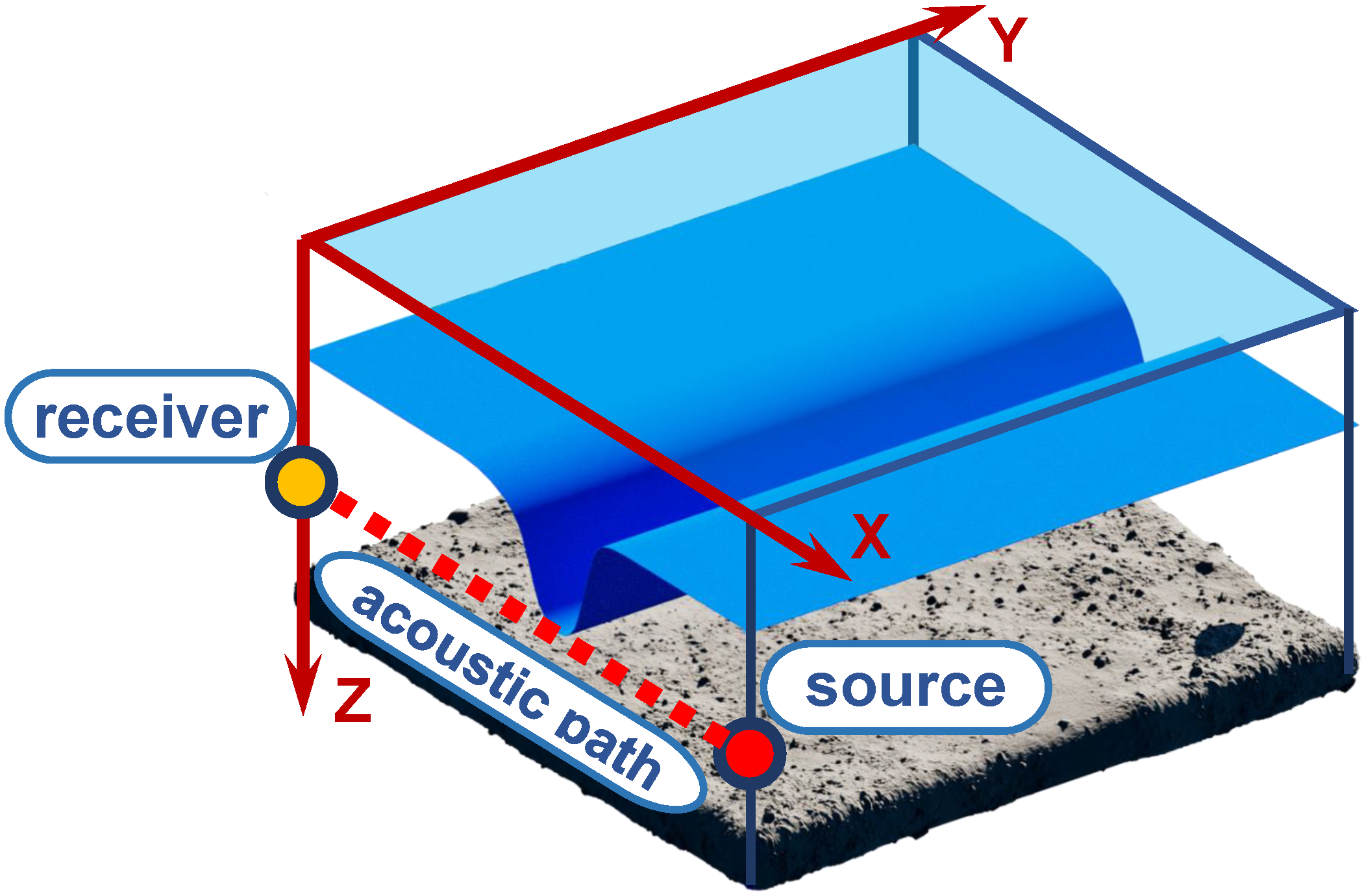
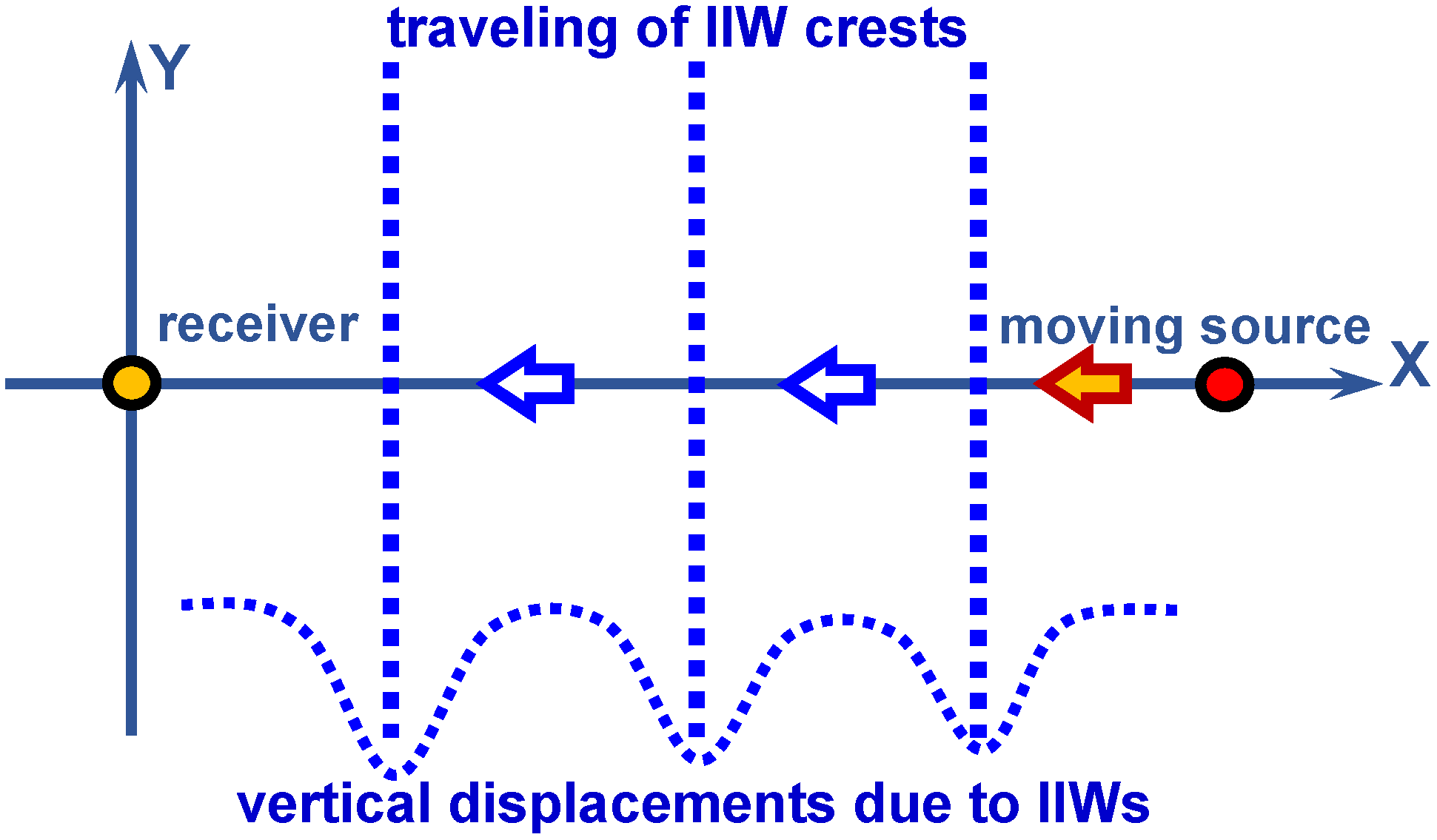
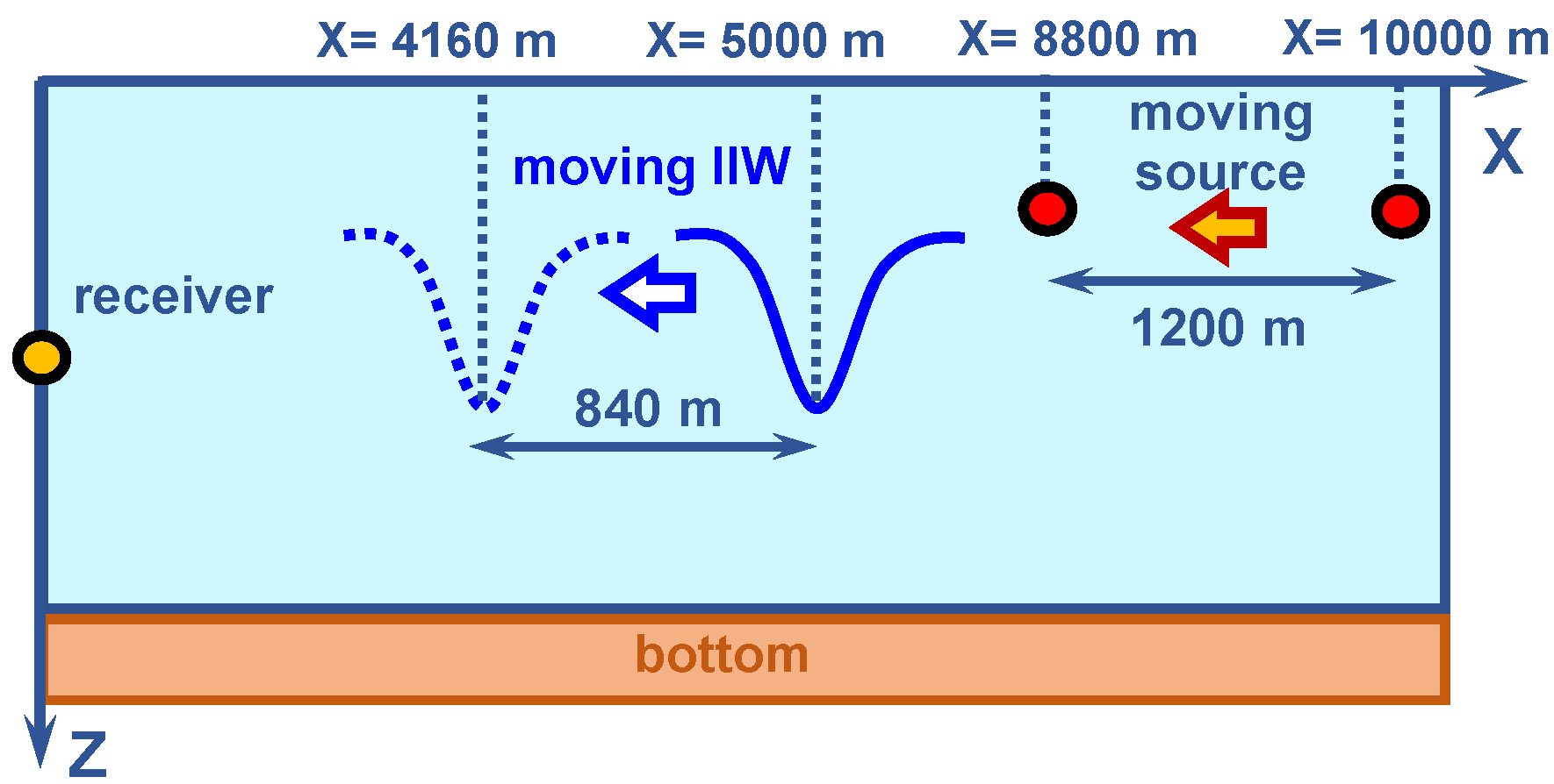
The geometries of the numerical simulations are shown in Figure 1 and Figure 2. IIWs travel along the acoustic path connecting the source and receiver. The internal soliton parameters are presented in

Table 5. Internal soliton parameters.

Parameter	Value
Amplitude	$B_n=15$ m
Width	${\eta }_n=150$ m
Velocity	$u_n=0.7$ m/s
Wavefront	$R=\infty$

. The amplitude is $B_n=15$ m, the width is 150 m, and the velocity is $u_n=0.7$ m/s. The wavefront is plane ($R=\infty$).

5.2. Results of Numerical Simulation—First Case: Non-Moving Source ($v=0$ m/s)

Consider the results of the numerical model for the first case, which is a non-moving source ($v=0$ m/s). The source–receiver range is $x_0=10$ km. The source depth is $z_s=12.5$ m. The receiver depth is $z_q=35$ m. The source spectrum is uniform. The sound pulses are recorded periodically at an interval of 5 s. The sampling frequency is $0.25$ Hz. The observation time is $T=20$ min. We consider the two frequency bands: $\Delta f_1=100$–120 Hz (Table 1) and $\Delta f_2=300$–320 Hz (Table 2).

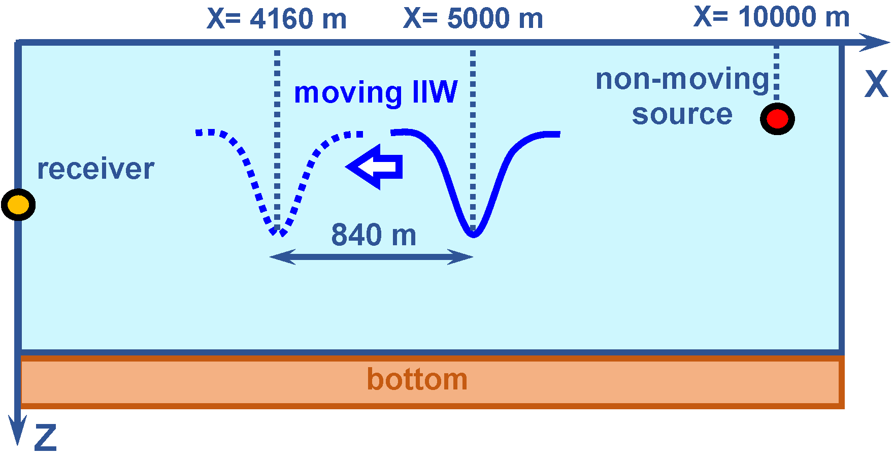
The numerical simulation model is shown in Figure 3. It is assumed that the intense internal waves (IIWs) are traveling along the acoustic path with a velocity of $u_n=0.7$ m/s from the source to the receiver. The IIWs are displaced by $\Delta x=840$ m during the $T=20$ min observation period. The initial position of the IIWs is $x=5000$ m. The final position of the IIWs is $x=4160$ m.

The outcomes of the numerical simulations are presented in Figure 4, Figure 5, Figure 6, Figure 7, Figure 8, Figure 9 and Figure 10. Figure 4 and Figure 5 illustrate the interferogram $I(f,t)$ and the corresponding hologram $F(\tau ,\tilde{\nu })$ in the absence of IIWs. Figure 4 represents the frequency band $\Delta f_1=100$–120 Hz, while Figure 5 refers to the frequency band $\Delta f_2=300$–320 Hz. The interferogram $I(f,t)$ is characterized by vertical, spatially localized fringes. The holographic representation $F(\tau ,\tilde{\nu })$ features focal points aligned along the horizontal axis, which is typical for a stationary (non-moving) sound source. As the frequency increases, both the structural complexity of $I(f,t)$ and the number of focal points in $F(\tau ,\tilde{\nu })$ grow. This effect is due to the greater number of propagating acoustic modes at higher frequencies (see Table 3 and Table 4).

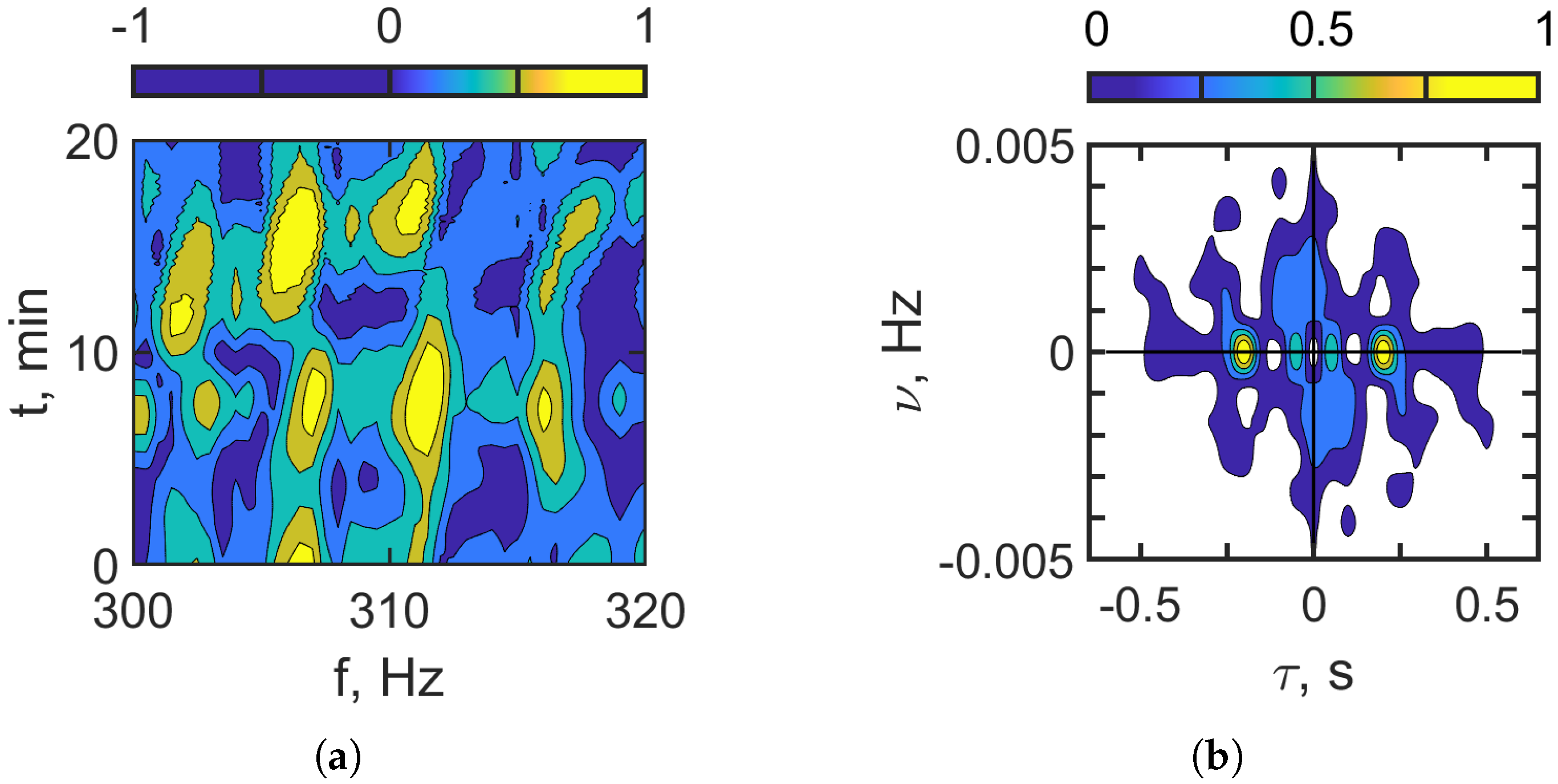
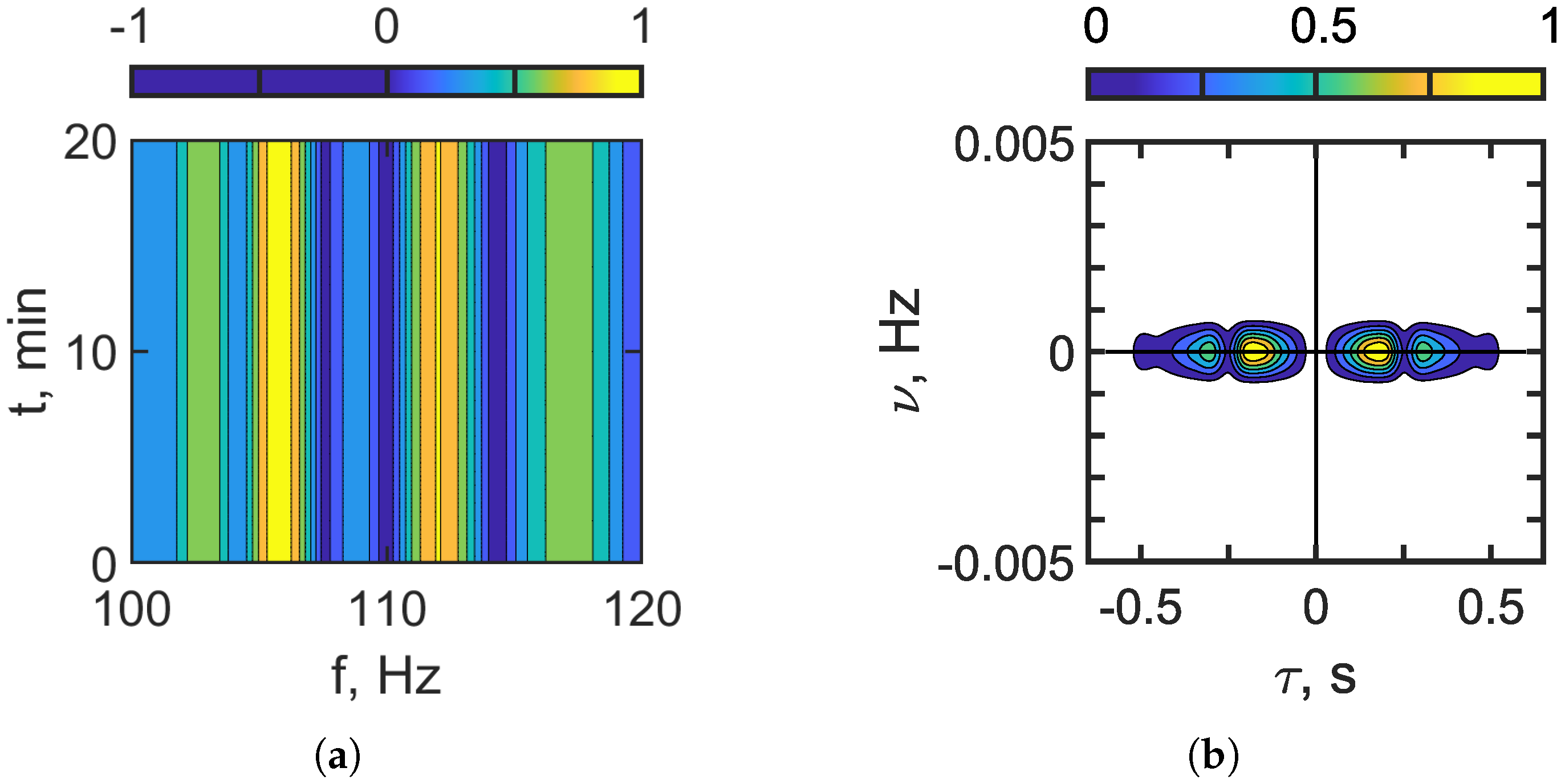
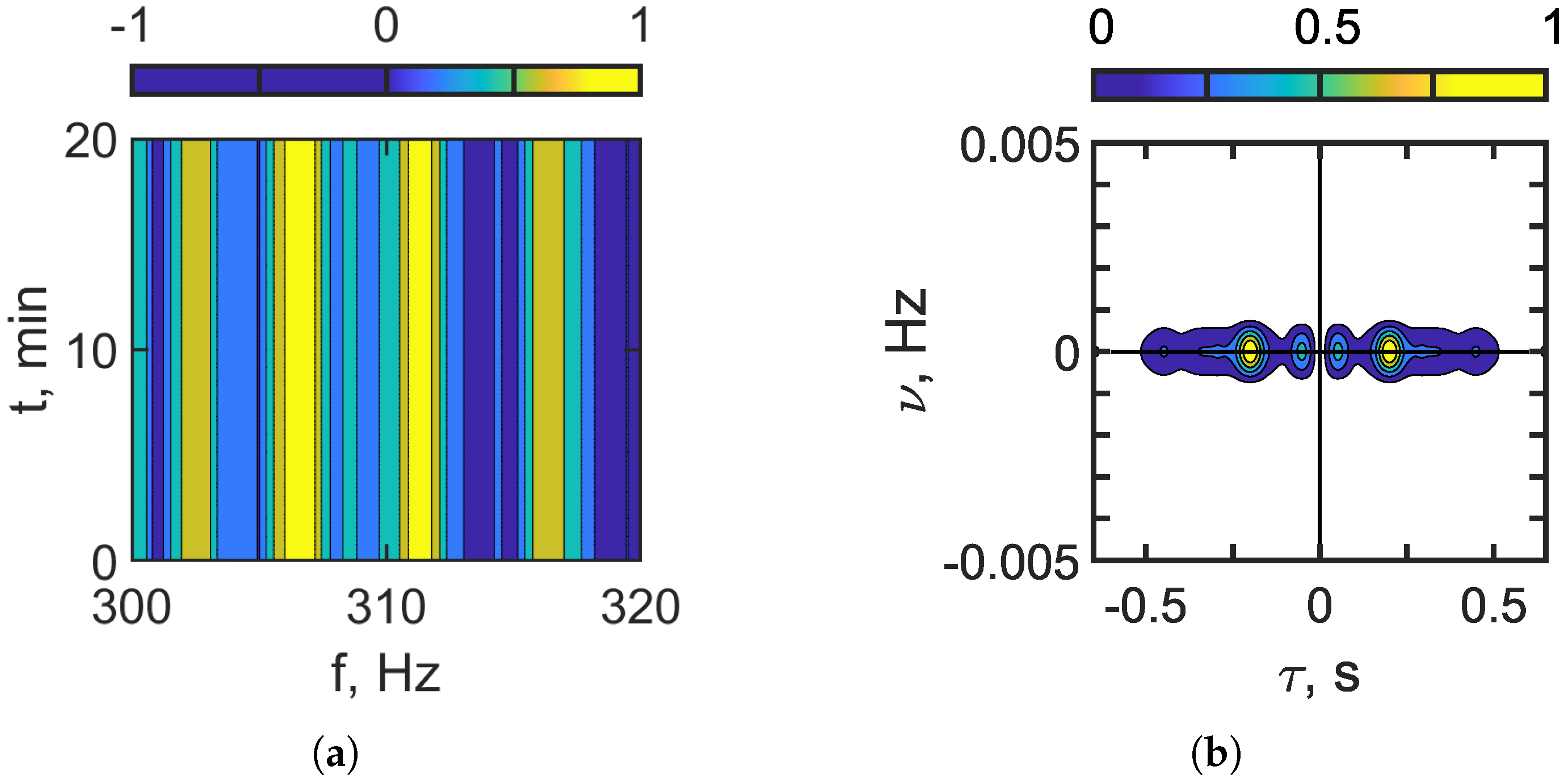
Figure 6 and Figure 7 show the interferogram $I(f,t)$ and the hologram $F(\tau ,\tilde{\nu })$ in the presence of IIWs. It is assumed that the IIWs travel along the acoustic path from the source to the receiver. Figure 6 corresponds to the frequency band $\Delta f_1=100$–120 Hz, and Figure 7 corresponds to $\Delta f_2=300$–320 Hz. In the lower-frequency range $\Delta f_1=100$–120 Hz, where mode coupling due to IIWs is weak, the resulting interferogram is dominated by vertically localized fringes (Figure 6a), which are characteristic of a shallow-water waveguide in the absence of IIWs. As the frequency increases to $\Delta f_2=300$–320 Hz, the effects of mode coupling caused by IIWs become more pronounced. The contribution of mode coupling to the sound field intensifies, resulting in the formation of horizontally localized fringes (Figure 7a). Consequently, the structure of the interferogram $I(f,t)$ becomes more complex.

Two types of focal spots appear in the hologram domain (see Figure 6b and Figure 7b). The focal spots that correspond to the vertical fringes of the interferogram $I(f,t)$, i.e., the shallow-water waveguide without IIWs, are concentrated along the time axis $\tau$. The focal spots that correspond to the horizontal fringes, i.e., the result of mode coupling due to IIWs, are concentrated along the frequency axis $\tilde{\nu }$. Outside of these focal spots, the spectral density is almost completely suppressed. Under natural conditions, an internal wave train (IIWT) consists of multiple internal solitons with varying parameters, which leads to a blurring of the distinct structure in both the interferogram $I(f,t)$ and the hologram $F(\tau ,\tilde{\nu })$. The arrangement of focal spots in the hologram $F(\tau ,\tilde{\nu })$ makes it possible to separate the component corresponding to the undisturbed waveguide from the component of the sound field that is perturbed by IIWs.

Figure 6. Interferogram $I(f,t)$ (a). Hologram $F(\tau ,\tilde{\nu })$ (b). Frequency band: $\Delta f_1=$ 100–120 Hz. Non-moving source: $v=0$ m/s. IIWs are present ($B_n=15$ m, $u_n=0.7$ m/s).

Figure 6. Interferogram $I(f,t)$ (a). Hologram $F(\tau ,\tilde{\nu })$ (b). Frequency band: $\Delta f_1=$ 100–120 Hz. Non-moving source: $v=0$ m/s. IIWs are present ($B_n=15$ m, $u_n=0.7$ m/s).

Figure 7. Interferogram $I(f,t)$ (a). Hologram $F(\tau ,\tilde{\nu })$ (b). Frequency band: $\Delta f_2=$ 300–320 Hz. Non-moving source: $v=0$ m/s. IIWs are present ($B_n=15$ m, $u_n=0.7$ m/s).

Figure 7. Interferogram $I(f,t)$ (a). Hologram $F(\tau ,\tilde{\nu })$ (b). Frequency band: $\Delta f_2=$ 300–320 Hz. Non-moving source: $v=0$ m/s. IIWs are present ($B_n=15$ m, $u_n=0.7$ m/s).

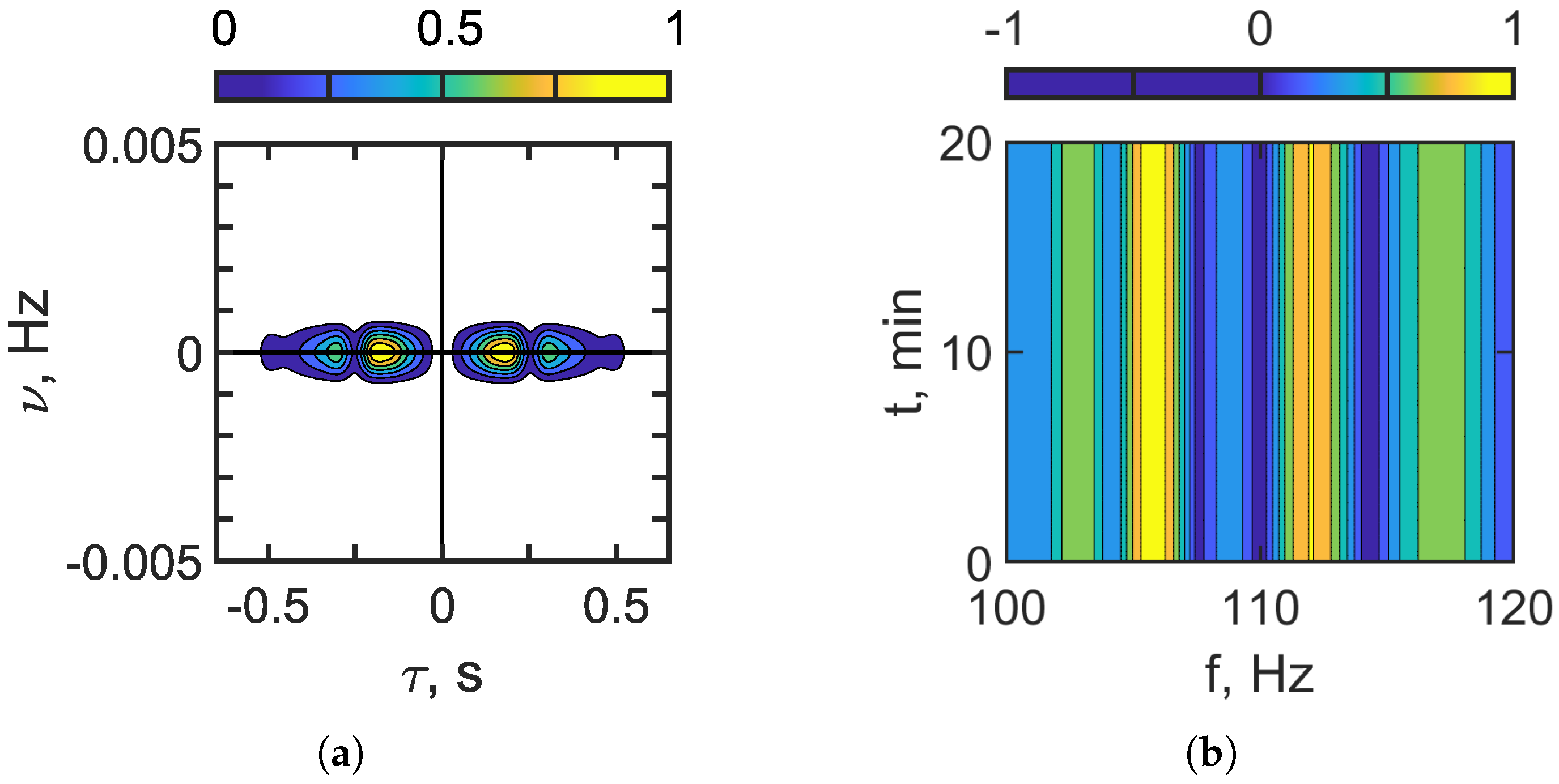
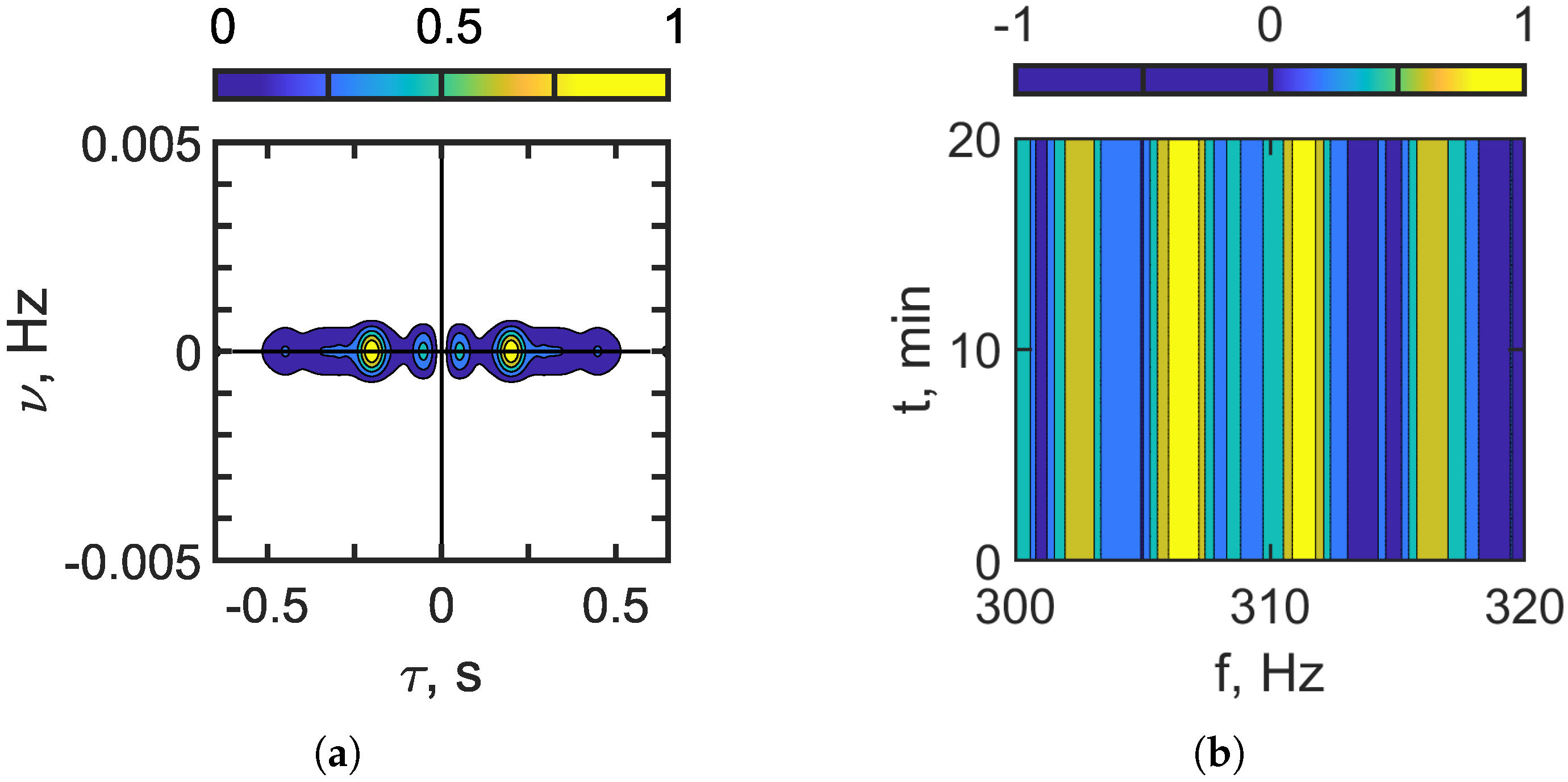
Figure 8 and Figure 9 present the results of applying a filter to the hologram to isolate the focal spots aligned horizontally in Figure 6 and Figure 7, followed by an inverse 2D Fourier transform (2D-FT) to obtain the corresponding interferograms. These interferograms and holograms (Figure 8 and Figure 9) closely resemble those representing the undisturbed waveguide scenario (without IIWs), as shown in Figure 4 and Figure 5. A comparison reveals that the positions and structures of the focal spots remain consistent between the original and reconstructed holograms. 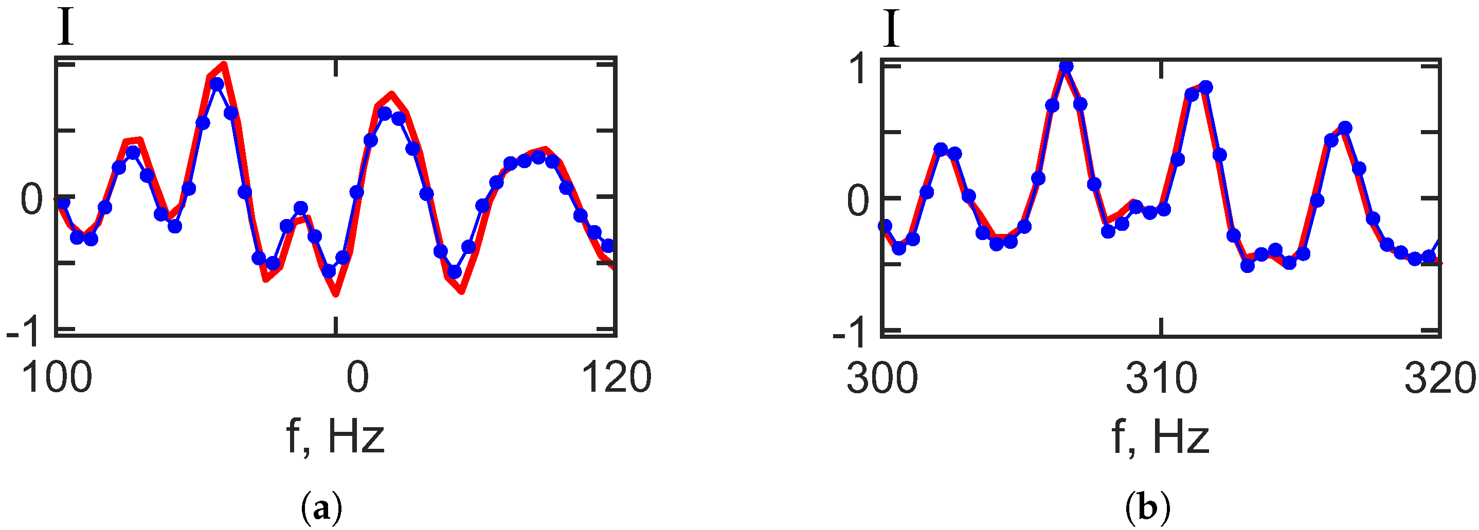Figure 10 provides further evidence by comparing one-dimensional slices of the two-dimensional interferograms $I(f,t)$ at a fixed time $t_0=0$ min. The red curve represents the case without IIWs, and the blue curve represents the case with IIWs, highlighting the similarity and confirming the effectiveness of the separation method.

Figure 8. Filtered hologram $F(\tau ,\tilde{\nu })$ (a). Filtered interferogram $I(f,t)$ (b). Frequency band: $\Delta f_1=$ 100–120 Hz. Non-moving source: $v=0$ m/s. IIWs are present ($B_n=15$ m, $u_n=0.7$ m/s).

Figure 8. Filtered hologram $F(\tau ,\tilde{\nu })$ (a). Filtered interferogram $I(f,t)$ (b). Frequency band: $\Delta f_1=$ 100–120 Hz. Non-moving source: $v=0$ m/s. IIWs are present ($B_n=15$ m, $u_n=0.7$ m/s).

Figure 9. Filtered hologram $F(\tau ,\tilde{\nu })$ (a). Filtered interferogram $I(f,t)$ (b). Frequency band: $\Delta f_2=$ 300–320 Hz. Non-moving source: $v=0$ m/s. IIWs are present ($B_n=15$ m, $u_n=0.7$ m/s).

Figure 9. Filtered hologram $F(\tau ,\tilde{\nu })$ (a). Filtered interferogram $I(f,t)$ (b). Frequency band: $\Delta f_2=$ 300–320 Hz. Non-moving source: $v=0$ m/s. IIWs are present ($B_n=15$ m, $u_n=0.7$ m/s).

Figure 10. Interferogram $I(f,t)$ slice ($t_0=0$ min) reconstructed by holographic filtering: (a) frequency band—$\Delta f_1=$ 100–120 Hz and (b) frequency band—$\Delta f_2=$ 300–320 Hz. Non-moving source: $v=0$ m/s. Red curve—IIWs are absent. Blue curve—IIWs are present ($B_n=15$ m, $u_n=0.7$ m/s).

Figure 10. Interferogram $I(f,t)$ slice ($t_0=0$ min) reconstructed by holographic filtering: (a) frequency band—$\Delta f_1=$ 100–120 Hz and (b) frequency band—$\Delta f_2=$ 300–320 Hz. Non-moving source: $v=0$ m/s. Red curve—IIWs are absent. Blue curve—IIWs are present ($B_n=15$ m, $u_n=0.7$ m/s).

The interferogram reconstruction error is estimated using the dimensionless quantity:

$$d={\displaystyle \frac{{\sum }_{j=1}^J\left|I_1\left(f_j\right)-I_2\left(f_j\right)\right|}{{\sum }_{j=1}^J\left|I_1\left(f_j\right)\right|}},$$

(30)

where $I_1\left(f\right)$ and $I_2\left(f\right)$ are the initial and reconstructed 1D interferograms, respectively. The interferogram reconstruction error values for the frequency bands $\Delta f_1=$ 100–120 Hz and $\Delta f_2=$ 300–320 Hz are presented in

Table 6. Interferogram reconstruction error values.

No.	$\mathbf{\Delta }{\mathit{f}}_1=100$–120 Hz	$\mathbf{\Delta }{\mathit{f}}_2=300$–320 Hz
1.	$d_1=0.014$	$d_2=0.074$
2.	$J=80$	$J=80$

.

The numerical modeling outcomes for the frequency band $\Delta f_2=300$–320 Hz are consistent with those obtained for the lower frequency range $\Delta f_1=100$–120 Hz. These results demonstrate that the proposed approach can separate the sound field into two components: one associated with the undisturbed waveguide and one resulting from the influence of IIWs. Consequently, it is possible to reconstruct the interferogram of the unperturbed waveguide even when the source is stationary and IIWs are present.

5.3. Results of Numerical Simulation—Second Case: Moving Source ($v=1$ m/s)

Consider the results of the numerical model for the second case, which involves a moving source ($v=1$ m/s). Initially, at $t_0=0$ min, the distance between the source and the receiver is set to $x_0=10$ km. The source is positioned at a depth of $z_s=12.5$ m, and the receiver is located at $z_q=35$ m. A uniform spectrum is assumed for the acoustic source. Each emitted sound pulse has a duration of $t_1=4$ s, with a sampling frequency of $0.25$ Hz. The interval between consecutive pulses is $t^{*}=5$ s, which includes a $t_2=1$ s pause after each pulse ($t^{*}=t_1+t_2$). The total observation time is $\Delta T=20$ min. Two frequency ranges are analyzed: $\Delta f_1=100$–120 Hz (Table 1) and $\Delta f_2=300$–320 Hz (Table 2).

The numerical simulation model is illustrated in Figure 11. It is assumed that IIWs propagate along the acoustic path from the source to the receiver at a velocity of $u_n=0.7$ m/s. During the observation period of $T=20$ min, the IIWs travel a distance of $\Delta x=840$ m. Their initial position is $x=5000$ m, and by the end of the observation period, they reach $x=4160$ m. During the same 20 min interval, the acoustic source moves horizontally along the x-axis toward the receiver at a constant speed of $v=1$ m/s, covering a distance of $\Delta x=1200$ m. The source’s initial location is $x=\mathrm{10,000}$ m, and its final position is $x=8800$ m.

Figure 12 and Figure 13 present the interferogram $I(f,t)$ and the corresponding hologram $F(\tau ,\tilde{\nu })$ for a moving source in the absence of intense internal waves (IIWs). Figure 12 illustrates the case for the frequency band $\Delta f_1=100$–120 Hz, Figure 13 refers to the frequency band $\Delta f_2=300$–320 Hz. The interferograms $I(f,t)$ are characterized by localized, slanted fringes. In the hologram domain, $F(\tau ,\tilde{\nu })$, the energy is concentrated in a series of focal spots in the I and III quadrants. As the frequency increases, both the complexity of the interferogram and the number of focal spots in the hologram grow, similar to the behavior observed with a non-moving source.

In the hologram domains in Figure 12b and Figure 13b, dashed lines are shown. These dashed lines indicate the region where the focal spots of the sound field in shallow water without IIWs are concentrated. The linear dimensions of this region are approximately $\delta \tau \approx 0.15$ s, $\delta \nu \approx 0.002$ Hz, which agrees with the theoretical focal spot dimension estimates, Equation (26): $\delta \tau =0.1$ s, $\delta \nu =0.0017$ Hz. The interferogram and hologram parameters for the case of a moving source and the absence of IIWs are presented in

Table 7. Interferogram and hologram structure parameters. Estimation of source parameters.

No.	$\mathbf{\Delta }{\mathit{f}}_1=100$–120 Hz	$\mathbf{\Delta }{\mathit{f}}_2=300$–320 Hz
1.	$\delta f/\delta t\approx -0.016$ s−2	$\delta f/\delta t\approx -0.035$ s−2
2.	${\tau }_1=1.0\times {10}^{-1}$ s	${\tau }_1=3.8\times {10}^{-1}$ s
3.	${\nu }_1=1.71\times {10}^{-3}$ Hz	${\nu }_1=2.0\times {10}^{-3}$ Hz
4.	$\dot{v}=0.99$ m/s	$\dot{v}=1.3$ m/s
5.	${\dot{x}}_0=9.1$ km	${\dot{x}}_0=11.1$ km

for the frequency bands: $\Delta f_1=100$–120 Hz and $\Delta f_2=300$–320 Hz.

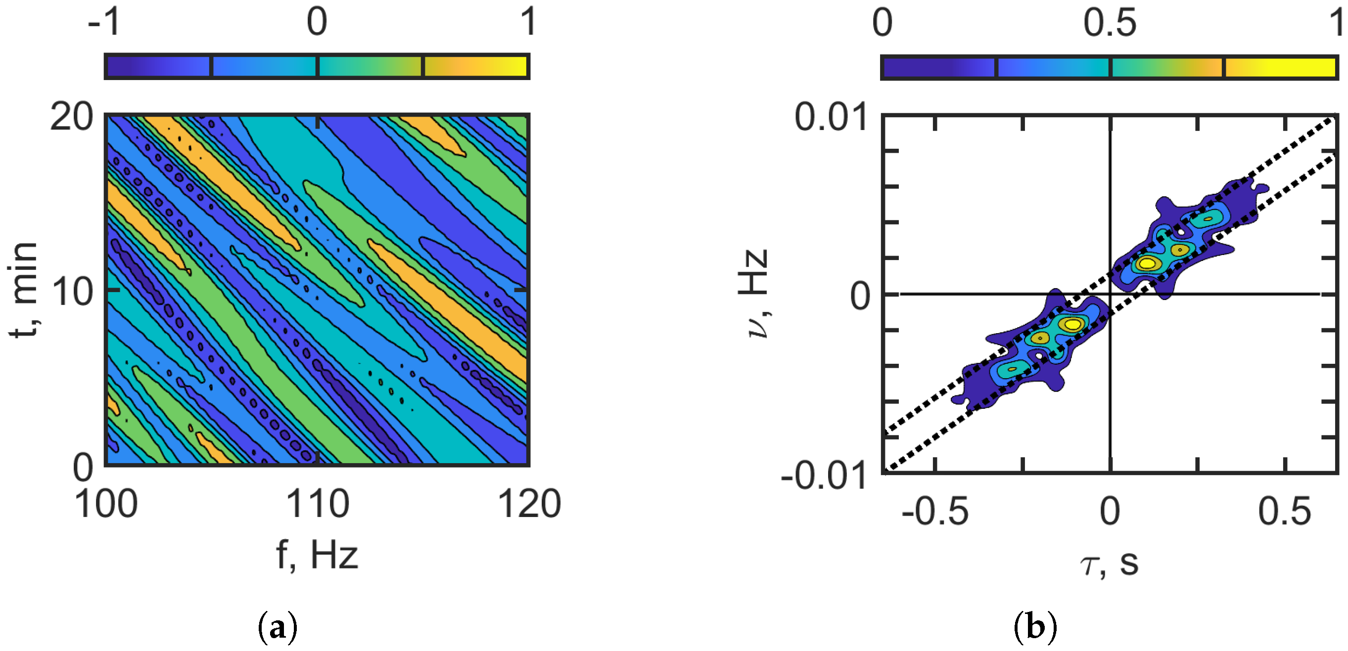
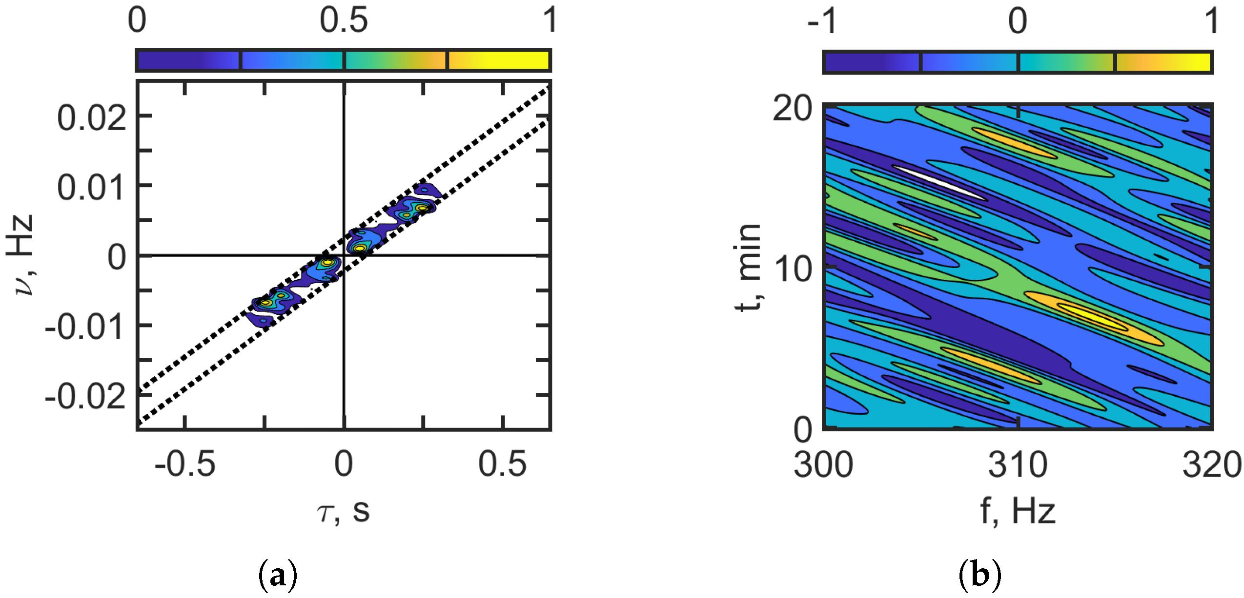
Figure 14 and Figure 15 show the interferogram $I(f,t)$ and the hologram $F(\tau ,\tilde{\nu })$ of the moving source in the case of IIWs traveling along the acoustic path between the source and the receiver. Figure 14 corresponds to $\Delta f_1=$ 100–120 Hz, and Figure 15 corresponds to $\Delta f_2=$ 300–320 Hz. Significant mode coupling due to IIWs leads to distortions of interferograms fringes $I(f,t)$ and the appearance of additional intense focal spots in the holograms $F(\tau ,\tilde{\nu })$ compared to the shallow-water waveguide without IIWs. The sound intensity along the interferogram fringes becomes highly nonuniform, taking the form of focal spots, as shown in Figure 14a and Figure 15a. This effect becomes more pronounced with an increasing frequency band. This is explained by the strengthening of the mode coupling effects due to the IIWs as the frequency increases. In the hologram domain, Figure 14b and Figure 15b, the concentration of focal spots along the frequency axis $\nu$ increases with the increase in the frequency band. This indicates the dominant influence of IIWs on the hologram structure.

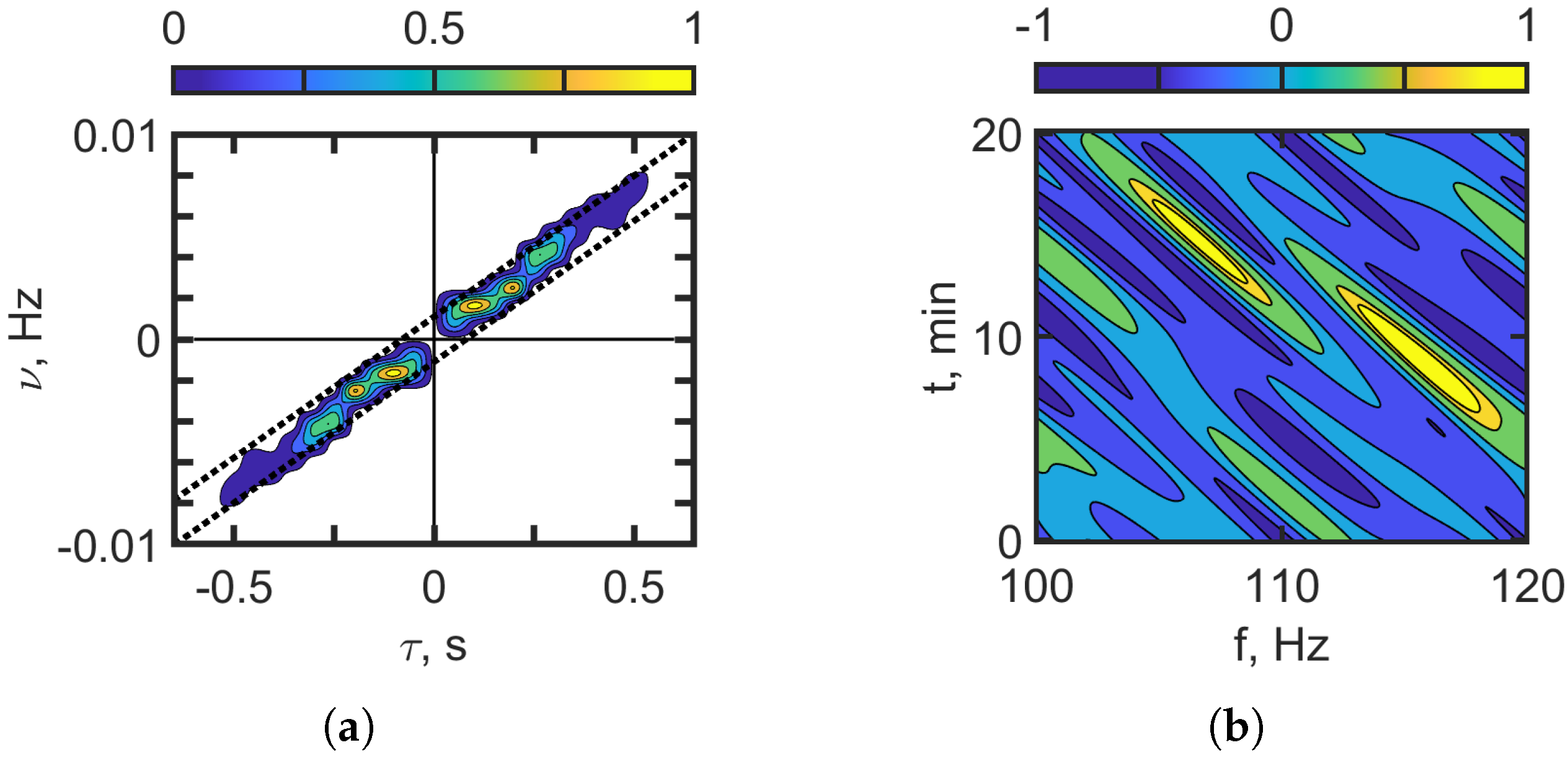
The spatial distribution of focal spots in the hologram $F(\tau ,\tilde{\nu })$ for a moving source allows one to distinguish between the component of the acoustic field component associated with an undisturbed waveguide and the component influenced by IIWs. Figure 14 and Figure 15 display the results of applying a filter to the focal spots located along the dotted lines in the holograms. The corresponding interferograms, obtained via inverse 2D-FT, are shown in Figure 16 and Figure 17. The reconstructed interferograms and holograms in these figures closely resemble those in Figure 12 and Figure 13, which show the case without IIWs. A comparison reveals that the positions of the focal spots in both the original and reconstructed holograms are nearly identical. The interferogram and hologram parameters for the case of a moving source and the presence of IIWs are presented in

Table 8. Interferogram and hologram structure parameters. Estimation of source parameters.

No.	$\mathbf{\Delta }{\mathit{f}}_1=100$–120 Hz	$\mathbf{\Delta }{\mathit{f}}_2=300$–320 Hz
1.	$\delta f/\delta t\approx -0.016$ s−2	$\delta f/\delta t\approx -0.035$ s−2
2.	${\tau }_1=1.19\times {10}^{-1}$ s	${\tau }_1=4.08\times {10}^{-1}$ s
3.	${\nu }_1=2.00\times {10}^{-3}$ Hz	${\nu }_1=1.63\times {10}^{-3}$ Hz
4.	$\dot{v}=1.1$ m/s	$\dot{v}=1.1$ m/s
5.	${\dot{x}}_0=10.8$ km	${\dot{x}}_0=12.0$ km

for the frequency bands $\Delta f_1=100$–120 Hz and $\Delta f_2=300$–320 Hz.

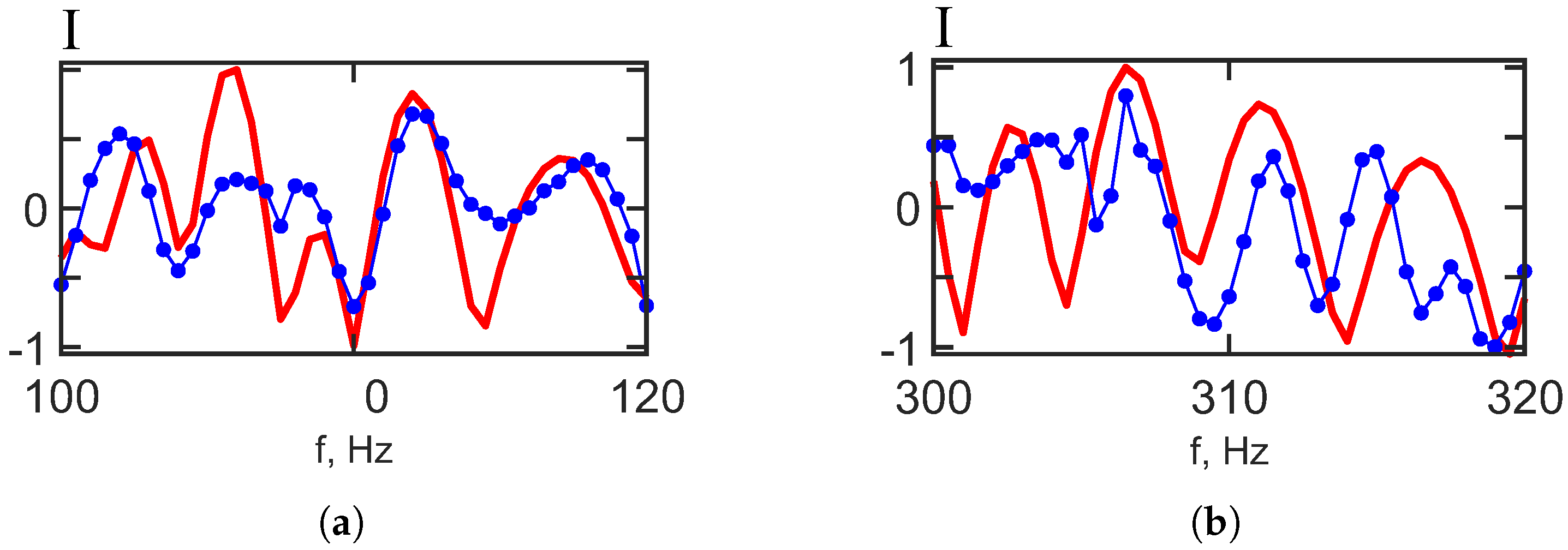
As can be seen, the focal spots on the reconstructed and initial holograms of the moving source are the same. Figure 18 shows the proximity of the initial and reconstructed interferograms of the moving source. Figure 18 shows the 1D interferograms for $t_0=0$ min. The red curve shows that IIWs are not present. The blue curve shows that IIWs are present. The interferogram reconstruction error values (Equation (30)) for the frequency bands $\Delta f_1=$ 100–120 Hz and $\Delta f_2=$ 300–320 Hz are presented in

Table 9. Interferogram reconstruction error values.

No.	$\mathbf{\Delta }{\mathit{f}}_1=100$–120 Hz	$\mathbf{\Delta }{\mathit{f}}_2=300$–320 Hz
1.	$d_1=0.635$	$d_2=0.821$
2.	$J=80$	$J=80$

.

Compared to the stationary source scenario, the reconstruction error for the frequency bands $\Delta f_1=100$–120 Hz and $\Delta f_2=300$–320 Hz increases by factors of $45.4$ and $11.1$, respectively. This suggests that reconstructing the interferogram of a waveguide without IIWs is less accurate when the source is in motion. The observed difference in error magnitudes arises from the varying nature of propagation conditions. While a stationary source is solely affected by variability introduced by IIWs, a moving source experiences additional variability due to its own motion, which compounds the effects of IIW-induced mode coupling.

The results of the numerical experiment demonstrated the robustness of the holographic method for detecting and localizing a moving underwater source in the presence of IIWs. The estimates of the source’s radial velocity and range were similar with and without IIWs. However, unlike with a stationary source, it is not possible to reconstruct the interferogram of the undisturbed field with a moving source when IIWs are present. The reconstruction error remains relatively high for a moving source. However, the angular slopes of the interference fringes are accurately recovered for both stationary and moving sources. The ability to accurately estimate the angular coefficients of the interference fringes during holographic reconstruction allows us to reliably determine the source parameters in both cases. For a moving source, the reconstructed parameter values are $\dot{v}=1.1\mathrm{m}/\mathrm{s}$ (error: 10%), $\dot{x}=10.8\mathrm{km}$ (error: 8%) for $\Delta f_1=100$–$120\mathrm{Hz}$; $\dot{v}=1.1\mathrm{m}/\mathrm{s}$ (error: 10%), $\dot{x}=12.0\mathrm{km}$ (error: 20%) for $\Delta f_1=300$–$320\mathrm{Hz}$.

6. Conclusions

We examined the robustness of the HSP method in the presence of intense internal waves (IIWs) for a moving, broadband source. We assumed that the IIWs traveled along the acoustic path between the source and receiver. Under these conditions, the IIWs cause significant scattering of sound intensity and mode coupling. Within the HSP framework, this study analyzes the interferogram—defined as the distribution of received sound intensity in the frequency–time domain—and its corresponding hologram, obtained via a 2D Fourier transform (2D-FT), for a moving source in the presence of space–time inhomogeneities caused by IIWs. A key result of the analysis is that, under the influence of IIWs, the hologram splits into two distinct regions representing the unperturbed and perturbed components of the acoustic field. This hologram structure allows us to extract and reconstruct the interferogram corresponding to the unperturbed field as if it existed in a shallow-water waveguide without IIWs.

We performed numerical simulations based on the VCMHR to evaluate the HSP method under realistic conditions, using the SWARM’95 experiment as a reference. The VCMHR accurately incorporates boundary conditions, captures the essential physics of vertical mode coupling due to environmental variability, and is well-adapted to low-frequency sound propagation in a shallow-water waveguide with IIWs. Several points should be highlighted regarding the limitations of our modeling approach. First, the shallow-water waveguide is represented with spatial and temporal variability introduced exclusively by IIWs. We acknowledge that the speed of sound propagation (approximately $1500\mathrm{m}/\mathrm{s}$) is significantly greater than the speeds of the moving source (approximately $0.5$–$5\mathrm{m}/\mathrm{s}$) and IIW propagation (approximately $0.5$–$1\mathrm{m}/\mathrm{s}$). Based on this, we employ the “frozen environment” approximation [41,60]. That is, the environment remains effectively unchanged during the relatively short time required for the acoustic signal to travel from the source to the receiver. This is a necessary advancement in the development of the HSP methodology. The numerical simulations performed provide a basis for a comparative analysis of the original and reconstructed source interferograms. The numerical simulation framework used in this study has been thoroughly validated using multiple experimental datasets, including SWARM’95, ASIAEX’01, and SHALLOW WATER’06, among others. In particular, its reliability was confirmed by processing and analyzing acoustic data collected during the SWARM’95 experiment [23]. The HSP technique was also verified using the SWARM’95 dataset [17,18,19,20]. We analyzed the SWARM’95 experimental dataset and found that, when IIWs are present, the hologram generated by the source separates into two parts. One part represents the waveguide conditions that are not perturbed, and the other part represents the perturbations that are induced by IIWs [17,18,19,20]. Unfortunately, the experiment did not allow for an assessment of the accuracy of source interferogram reconstruction under conditions without IIWs because such data were unavailable. Consequently, the present study is a critical advancement in the development of the HSP methodology. The numerical simulations performed provide a basis for a comparative analysis of the original and reconstructed source interferograms.

Within the framework of the numerical simulations, two frequency bands are considered: $\Delta f_1=100$–120 Hz and $\Delta f_2=300$–320 Hz. The IIWs propagate along the acoustic path at a velocity of $0.7\mathrm{m}/\mathrm{s}$. The study considers a stationary source with a velocity of $0\mathrm{m}/\mathrm{s}$ and a moving source with a velocity of up to $1\mathrm{m}/\mathrm{s}$). High reconstruction accuracy is achieved with error values as low as $d_1=0.014$ for the first frequency band $\Delta f_1=100$–120 Hz and $d_2=0.074$ for the second frequency band $\Delta f_2=300$–320 Hz in the case of a stationary source. However, compared to the stationary source, the reconstruction error increases for the moving source scenario: $d_1=0.635$ for ($\Delta f_1=100$–120 Hz) and $d_2=0.821$ for ($\Delta f_2=300$–320 Hz). The reconstruction errors increase by factors of $45.4$ and $11.1$. The difference in error magnitudes is explained by variations in propagation conditions. For a stationary source, the received acoustic field is only affected by fluctuations caused by IIWs, making this the most favorable scenario for holographic reconstruction. In contrast, when a moving source travels in the same direction as the IIWs at a similar speed, the acoustic field is influenced by the variability introduced by the source’s motion. This makes accurate holographic reconstruction the most challenging in this situation. Thus, we can conclude that the error in holographic reconstruction in other cases will lie between the following values: $0.014\le d_1\le 0.635$ and $0.074\le d_1\le 0.821$. As our results show, holographic reconstruction error depends on frequency. For the higher-frequency band, the reconstruction error increases. This is because mode coupling becomes more significant and internal waves distort the acoustic field more strongly at higher frequencies. This phenomenon has been noted in papers regarding the influence of IIWs on the sound field (see [52]).

In summary, our study’s results support the assertion that the developed HSP approach is a viable alternative to the widely used MFP technique [61,62,63,64,65]. Although MFP has been extensively applied in underwater acoustics, its practical implementation is constrained by several critical factors. Specifically, MFP necessitates precise and detailed knowledge of the propagation environment, including comprehensive information about the structure of the water column and the properties of the seabed [61,62]. In contrast, the HSP method is more robust in the face of environmental uncertainties and can operate effectively without prior knowledge of the waveguide. This makes it a promising tool for real-time, adaptive acoustic sensing in complex, dynamic ocean environments [65]. Our research advances signal processing methods in underwater acoustics by introducing efficient HSP methods for environments with spatiotemporal inhomogeneities. Future research will focus on the influence of irregular bathymetry on hologram reconstruction of a moving source in shallow water.