Abstract
This paper investigates the pressure fluctuation characteristics induced by cavitation in the blade-tip region of an axial flow pump through experimental and numerical methods. Compared with previous studies, this research not only analyzes the development of cavitation bubbles under varying flow rates but also explores the transient pressure fluctuation features caused by cavitation. It is found that partial-loading conditions tend to exacerbate cavitation, leading to more pronounced transient flow characteristics. The primary frequency of pressure fluctuations consistently corresponds to the impeller’s rotational frequency and its harmonics, with the magnitude inversely related to flow rate. At the same cavitation stage, lower flow rates exhibit larger amplitudes and more significant fluctuations in high-frequency components. This indicates stronger entrainment disturbance between the cavitation morphology and the mainstream in the blade-tip region at lower flow rates, resulting in more complex flow structures. This study provides a theoretical basis for understanding the mechanisms of pressure fluctuations induced by cavitation in the blade-tip region of axial flow pumps.
1. Introduction
Axial flow pumps, as a blade-type piece of hydraulic machinery, are widely used in large-scale water transfer projects and propulsion systems of ships and submarines, which benefit from their advantages of large flow rate and high efficiency [1]. Axial flow pumps exhibit structural features that create a space between the impeller and the runner chamber wall. During blade operation, the pressure differential between the pressure and suction surfaces drives leakage flow through the tip clearance. Upon merging with the suction-side mainstream flow, this leakage flow develops into a distinct tip leakage vortex (TLV) [2]. When a TLV occurs, low-pressure areas can induce the formation of vortex cavitation. Severe cavitation may cause hydraulic excitation and noise, leading to the deterioration of pump performance [3,4,5,6,7].
Researchers have engaged in pertinent investigations pertaining to the cavitation phenomena occurring in axial flow pumps. In 1954, Rains [8] first observed tip leakage vortex cavitation at the blade tip of an axial flow pump. Katz et al. [9] investigated the temporal and spatial characteristics of the evolution of cavitation structures in water-jet propulsion axial flow pumps using high-speed photography experiments. Tabar et al. [10,11] also conducted visualization experiments to study tip clearance cavitation in axial flow pumps under different flow conditions. They compared the effects of different flow rates and outlet pressure conditions on TLV cavitation. Laborde et al. [12] delved into a comprehensive examination of how various blade designs, rotation rates, and spacing factors influence tip clearance cavitation within axial flow pumps. Notably, they highlighted that spacing dimensions play a pivotal role in the formation of tip cavitation in these pumps. To address this challenge, researchers have proposed several mitigation techniques for tip leakage cavitation, including blade angle optimization and leading-edge rounding of the impeller. Tan et al. [13] investigated the complex cavitation structures within axial flow pumps. They identified the perpendicular cavitation vortices (PCVs) that originate from the edge of the cavitation cloud on the suction side of the preceding blade and extend towards the pressure side of the next blade. Zhang and team [14] took a closer look at the factors contributing to the formation of tip leakage vortices and the role of gap size. Through a combination of experiments and computations, they determined that the leakage shear layer is the primary site for vortex formation. The axial mainstream and gap jet create convection, which enhances the formation and development of vortices. Larger gaps lead to increased leakage velocities and larger tip leakage vortex (TLV) scales [15].
Pressure fluctuation serves as a crucial indicator of pump stability. The process of cavitation and its progression are often marked by changes in the temporal and spectral characteristics of pressure wave signals. Therefore, it is essential to investigate how cavitation influences the internal pressure pulsations within the rotor of an axial flow pump. Understanding this relationship is crucial for enhancing the operational reliability of the pump. Many scholars have conducted research on the pressure fluctuations caused by cavitation. Zhang et al. [16] utilized the root-mean-square (RMS) technique to delve into how the energy intensity of pressure pulsation shifts during cavitation. Their findings indicate that the signature peaks of the root mean square (RMS) provide superior predictive capability for identifying cavitation compared to the conventional 3% head drop threshold. The energy characteristics of pressure fluctuations allow for a more accurate and timely determination of cavitation occurrence. Liu et al. [17] examined how cavitation develops and how pressure fluctuations behave during the startup phase of a centrifugal pump. Their research revealed that as the impeller accelerated, both the intensity and rate of pressure fluctuations grew significantly. During this transient operation, the mean pressure at the impeller inlet decreased to vaporization levels, leading to a significant increase in vapor concentration. Zhou et al. [18] conducted numerical simulations of the pressure fluctuations caused by cavitation flow in an orbital pump. Their study revealed that as the inlet pressure decreased, the cavitation within the orbital pump intensified and the severity of cavitation in the rotor increased. Furthermore, some vapor infiltrated into the oil inlet chamber, resulting in a significant increase in the vapor concentration within the space where it interacts with the oil inlet. Gong et al. [19] developed an integrated experimental setup featuring high-speed cameras and precision sensors to analyze the pressure variations and mechanical vibrations caused by tip-leakage vortex (TLV) cavitation. Their findings revealed that the emergence of TLV cavitation clouds substantially impaired pump efficiency, disrupted normal pressure patterns, and amplified both pressure oscillations and structural vibrations. Shen et al. [20] conducted an examination into how tip leakage cavitation and perpendicular vortex cavitation influence the variations in pressure within axial flow pumps. The study revealed that as perpendicular cavitation vortices move towards neighboring blades and interact with the TLV, they cause pressure fluctuations during the pressure recovery process. Zhang et al. [21] conducted numerical simulations to study the cavitation flow and its induced pressure fluctuation characteristics in axial flow pumps. The results showed that under cavitation conditions, the dominant frequency of the pressure fluctuation at the impeller outlet was the blade passage frequency and that the harmonic frequencies were multiples of the blade passage frequency. As the cavitation number reduced, a notable augmentation in the magnitude of pressure fluctuations was observed. Li et al. [22,23] investigated the dynamics of pressure variations and vibrations associated with cavitation at the blade tips in an axial flow pump. They found that such cavitation can cause intense pressure spikes and distinct vibrational characteristics. Feng et al. [24] observed that the presence of gap flow had the effect of amplifying the magnitude of pressure fluctuations within the impeller.
A review of the relevant literature indicates that the phenomenon of pressure fluctuation caused by cavitation in the tip region has consistently attracted considerable attention in the field of axial flow pumps. Research on the comparative analysis of numerical simulations and experimental data regarding the pressure fluctuation characteristics in axial flow pumps under varying cavitation conditions remains relatively limited. Building on these insights, this paper investigates the development of cavitation bubbles within the impeller of an axial flow pump and the transient pressure fluctuations induced by these bubbles in the blade-tip region. This investigation is conducted by merging computational methods and hands-on experiments. It provides a theoretical basis for in-depth research on the generation mechanisms of unstable pressure fluctuation induced by tip leakage vortices and cavitation.
2. Materials and Methods
2.1. Geometric Model
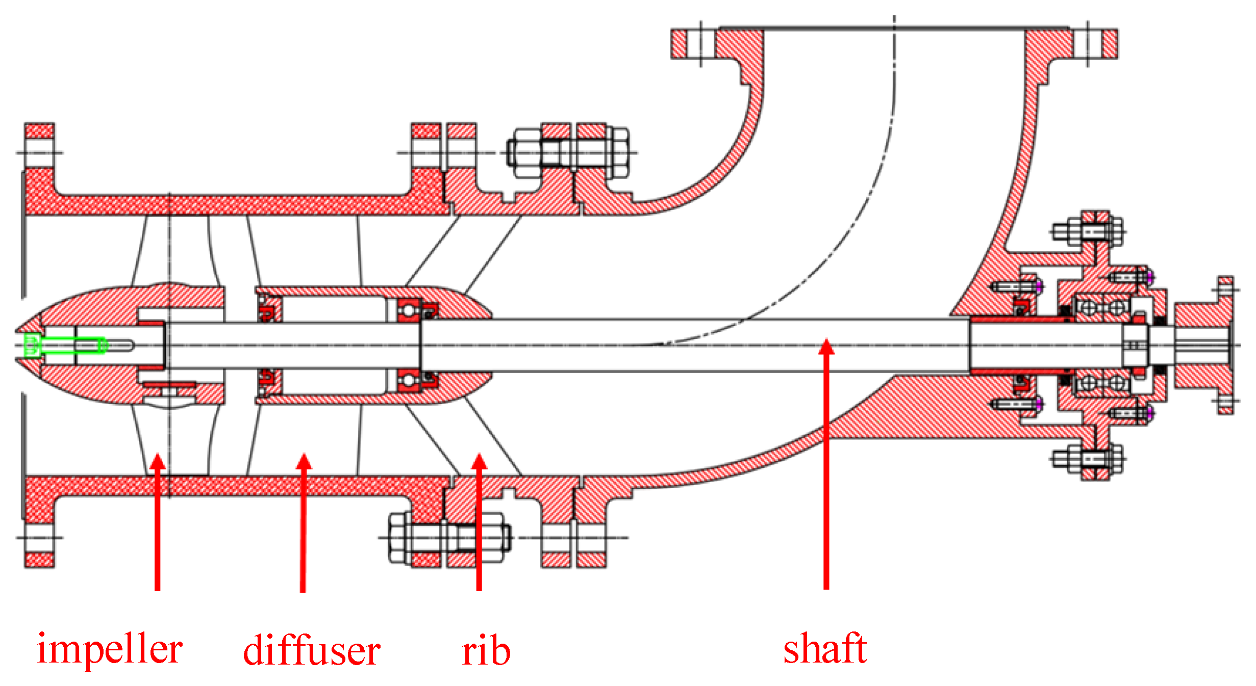
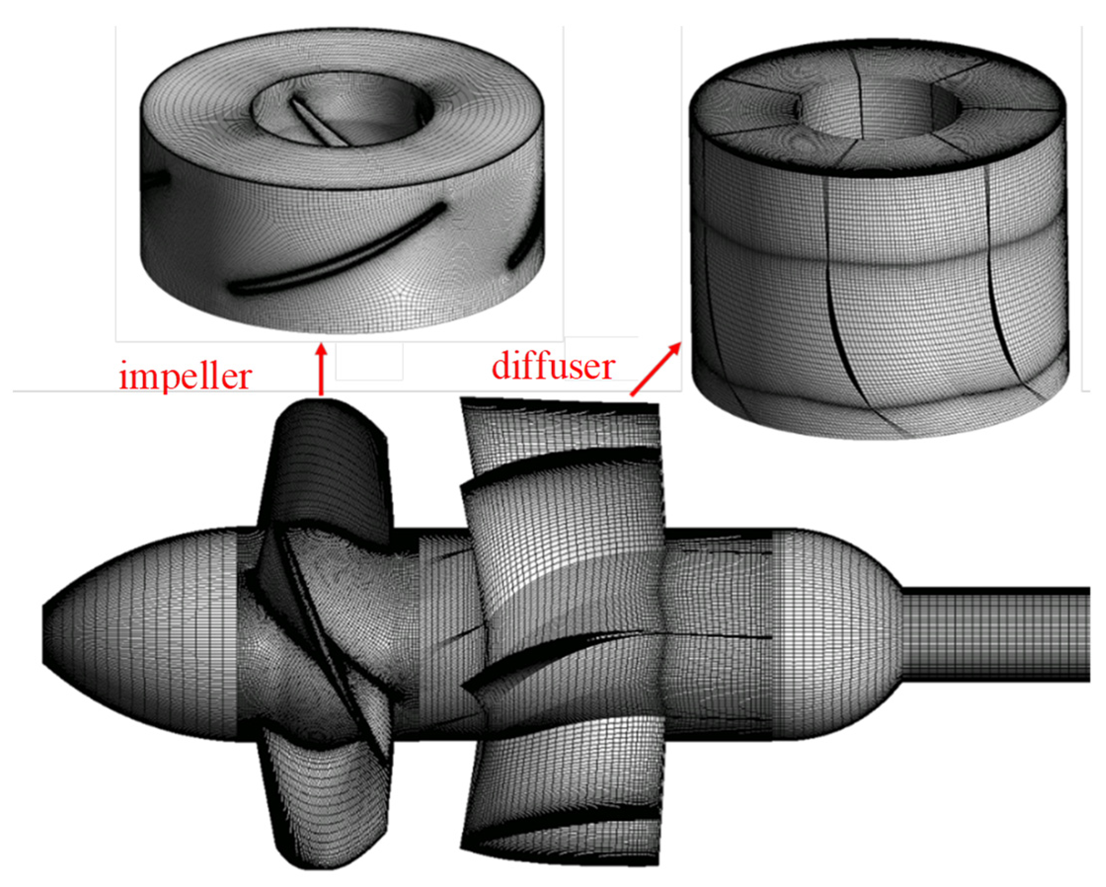
The study focuses on a scaled version of the TJ04-ZL-02 axial flow pump utilized in the South-to-North Water Diversion Project. The prototype was manufactured by Tianjin Pump Industry Co., Ltd., located in Tianjin, China. Figure 1 shows a scale model of the hydraulic components. The parameters of the model pump are shown in Table 1 [20].

Figure 1.
Computational domain of the axial flow pump.

Table 1.
Main design parameters of model pump.
2.2. Turbulence Model
The Partially-Averaged Navier–Stokes (PANS) turbulence model, proposed by Girimaji [25], is a hybrid approach capable of smoothly transitioning from the Reynolds-Averaged Navier–Stokes (RANS) method to Direct Numerical Simulation (DNS). The PANS framework regulates the transition via the fk, defined as the ratio of unresolved turbulent kinetic energy to the total turbulent kinetic energy. Its advantage lies in its ability to directly resolve the turbulent flows of varying scales in local regions. As fk approaches unity in high-resolution regions remote from solid walls, the PANS model asymptotically reverts to a DNS-like regime, thereby resolving the majority of turbulent fluctuations directly. Conversely, as fk tends to zero in low-resolution near-wall regions, the model reduces to a conventional RANS mode, with turbulence effects entirely subsumed by the closure model. The fundamental Equations (1)–(8) have been widely applied in simulating unsteady cavitating flows [26,27].
fk represents the ratio of unresolved turbulent kinetic energy to the total turbulent kinetic energy:
Closure function fε equation:
Based on the k-ε model, the turbulence kinetic energy and dissipation equations of the PANS model are as follows:
In the equation, represents the unresolved scale production term, with and are defined as follows:
In the present research, modifications are made to the source terms of the standard k-ε turbulence model through the application of secondary development methodologies within CFX. Specifically, the embedded PANS model was incorporated into the transient cavitation calculations of the axial flow pump being studied. For high-Reynolds-number flows, according to reference [28], fε = 1.0. The value of fk significantly affects the results of unsteady cavitation simulations. Based on references [26,27], fk = 0.4 is adopted in the present study, ensuring that the high-frequency fluctuations of tip-leakage cavitating vortices are adequately resolved while the near-wall regions remain in a RANS mode for computational efficiency.
2.3. Cavitation Model
The cavitation model, grounded in the Rayleigh–Plesset equation and homogenous in nature, is utilized within the Zwart–Gerber–Belamri framework. The model assumes that the gas–liquid two-phase flow is a homogeneous and incompressible fluid. Additionally, it assumes that there is no slip motion between the two phases. The fundamental equations encompassing the continuity equation, momentum equation, and transport equation are employed to model the transition of phases between liquid and gas. These equations serve as the basis for simulating such processes.
The Rayleigh–Plesset equation describes the growth process of a single bubble in a liquid phase:
where is the bubble radius, mm; is the saturated vapor pressure, Pa; and is the liquid–vapor surface tension coefficient. Typically, the effects of the surface tension term, viscous term, and second-order derivative differential term are neglected, and the equation is expressed as
The rate of mass transport for a single bubble is
As the vapor volume fraction increases, the nucleation density correspondingly decreases. During the evaporation process, assuming that the number of bubbles per unit volume remains constant, replaces . Assuming that the number of bubbles per unit volume remains constant is denoted as . Therefore, the gas-phase volume fraction can be expressed as
The interphase volumetric mass transfer rate is
The mass transport process between the vapor and liquid phases, which characterizes evaporation and condensation, can be represented as in Refs. [29,30]:
2.4. Grid Generation and Numerical Settings
2.4.1. Grid Generation
Before conducting numerical simulations, the model must be discretized into a mesh. The accuracy of the simulation depends on the quality of the computational mesh. The impeller design of the pump model is particularly complex. Local mesh refinement in the tip clearance and boundary layer zones is accomplished using hexahedral structured grids, which meet the wall function requirements of the turbulence model. This enables a more precise calculation and forecasting of the intricate flow patterns within the tip region, subsequently enhancing the accuracy of the computational results. In this paper, the preprocessing module ICEM in ANSYS 19.2 is used to discretize the computational domains into hexahedral structured meshes. As shown in Figure 2, the inlet section, rib, elbow pipe, and outlet section adopt an O-type topological structure, while the guide vane adopts an H-type topological structure. For the key hydraulic components of the impeller, the turbogrid meshing module is used to perform structured meshing. The mesh element counts for the inlet section, rib, elbow pipe, and outlet section are 540,432, 356,184, 354,913, and 521,652, respectively. The impeller and diffuser grids comprise 7,067,531 and 3,324,315 elements, correspondingly. As illustrated in Figure 3, the presentation encompasses the distribution of y+ values across the pressure surface, the suction surface of the blade, as well as the wall of the runner chamber. The y+ values on the blade surface lie between 1 and 20, with an average y+ of 7 in the end-wall region of the tip clearance, ensuring that fk remains sufficiently low for the near-wall region to operate in a RANS mode. In conjunction with the prescribed fk = 0.4 in Section 2.2, this configuration ensures that the flow regions remote from the wall are resolved in a DNS-like manner.
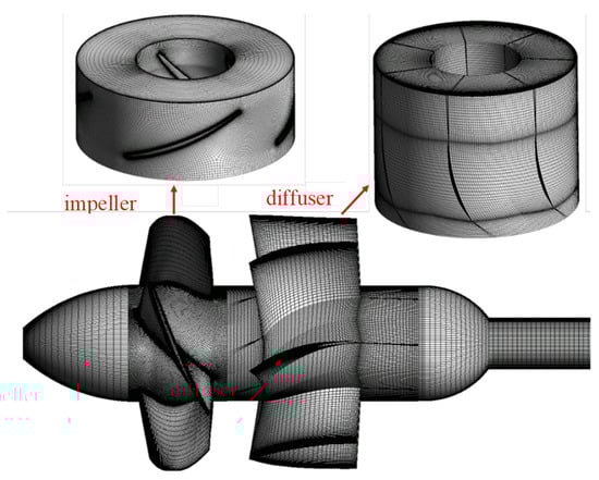
Figure 2.
Mesh for the entire flow field computational domain.
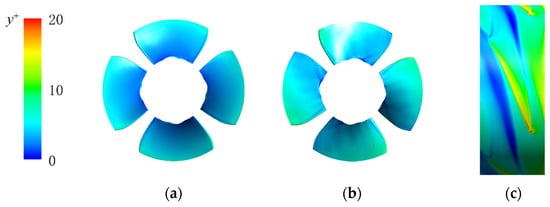
Figure 3.
Distributions of y+ on blade surfaces and rotor chamber wall: (a) pressure surface; (b) suction surface; (c) rotor chamber.
2.4.2. Boundary Condition Settings
The impeller constitutes the rotating region, spinning at 1450 r/min. The fluid domains, with the exception of the rotating impeller, are configured as static domains with a reference pressure of 0 atm. The inlet is configured with a specified total pressure of 1 atm. During cavitation calculations, to induce cavitation within the pump, the inlet pressure is decreased. The vapor phase and its saturation pressure are both set at 3574 Pa. The outlet is configured to have a mass flow rate of Q = 101.4 kg/s, which is based on the actual flow rate. The interfaces between different computational domains are connected using the General Grid Interface (GGI) mode. For steady-state and transient simulations, the types of rotor–stator interfaces are “Frozen Rotor” and “Transient Rotor Stator”, respectively. The transient analysis employs the steady-state outputs as starting points, with the computation for 10 rotations taking 0.414 s. Each time step corresponds to a 2° rotation of the impeller, with a time interval of t = 2.30 ms. The convergence criteria for steady-state and transient simulations are set to 1 × 10⁻⁵, respectively. The stable results from the last few revolutions of the transient simulation are used for analysis.
2.5. Analysis of Mesh Discretization Error
The quality and quantity of the mesh elements are crucial factors in determining the accuracy and reliability of the numerical results. Therefore, it is necessary to conduct an analysis of mesh discretization error. Increasing mesh elements in the solution domain enhances simulation accuracy and precision. However, an excessive number of mesh elements can significantly increase the computational cost. Therefore, it is necessary to determine a reasonable mesh for the computational domain in advance to balance computational accuracy and resource utilization. In this study, the criterion of the Grid Convergence Index (GCI), which relies on the Richardson Extrapolation (RE) technique [30], is employed to ascertain the validity of the mesh. This allows for the determination of the optimal computational mesh scheme. Consequently, three mesh schemes (N1, N2, and N3) with sparse, medium, and fine resolutions are selected for the entire computational domain. The ψ and η, serving as two pivotal performance parameters, are used as indicators to assess mesh error.
The head coefficient of the pump ψ is denoted as
The formula for pump efficiency η [15] is
where ρ is fluid density, kg/m3; Q is flow rate, m3/h; H is pump head, m; and M is torque, N m.
A grid discretization error analysis was conducted for operating conditions ranging from Q/Qopt = 1.2 to Q/Qopt = 0.8, with corresponding Φ values of 0.63, 0.52, and 0.42, respectively. As shown in Table 2, the main parameters include grid refinement ratio r, solution parameters ϕ, extrapolated solution value ϕext21, relative of the extrapolated value eext21, and fine grid convergence metric GCIfine21. Analysis of the grid error results reveals that increasing the number of grid points leads to improvements in solution accuracy and y+ values, resulting in enhanced computational precision. However, an excessive number of grid points will increase the computational time period and the computational resource cost. Consequently, N2 = 12,549,278 was ultimately selected as the grid scheme for the numerical simulations presented in this paper.
Table 2.
Results of mesh discrete error analysis [31].
2.6. Experimental Setup and Methods
2.6.1. Experimental Setup and Model Pump
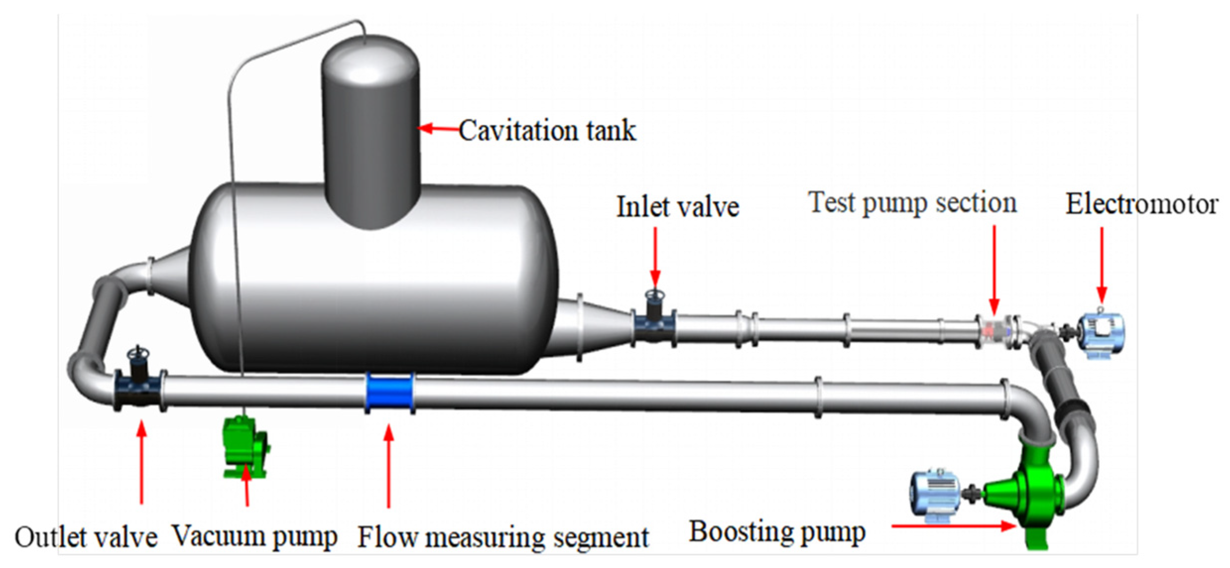
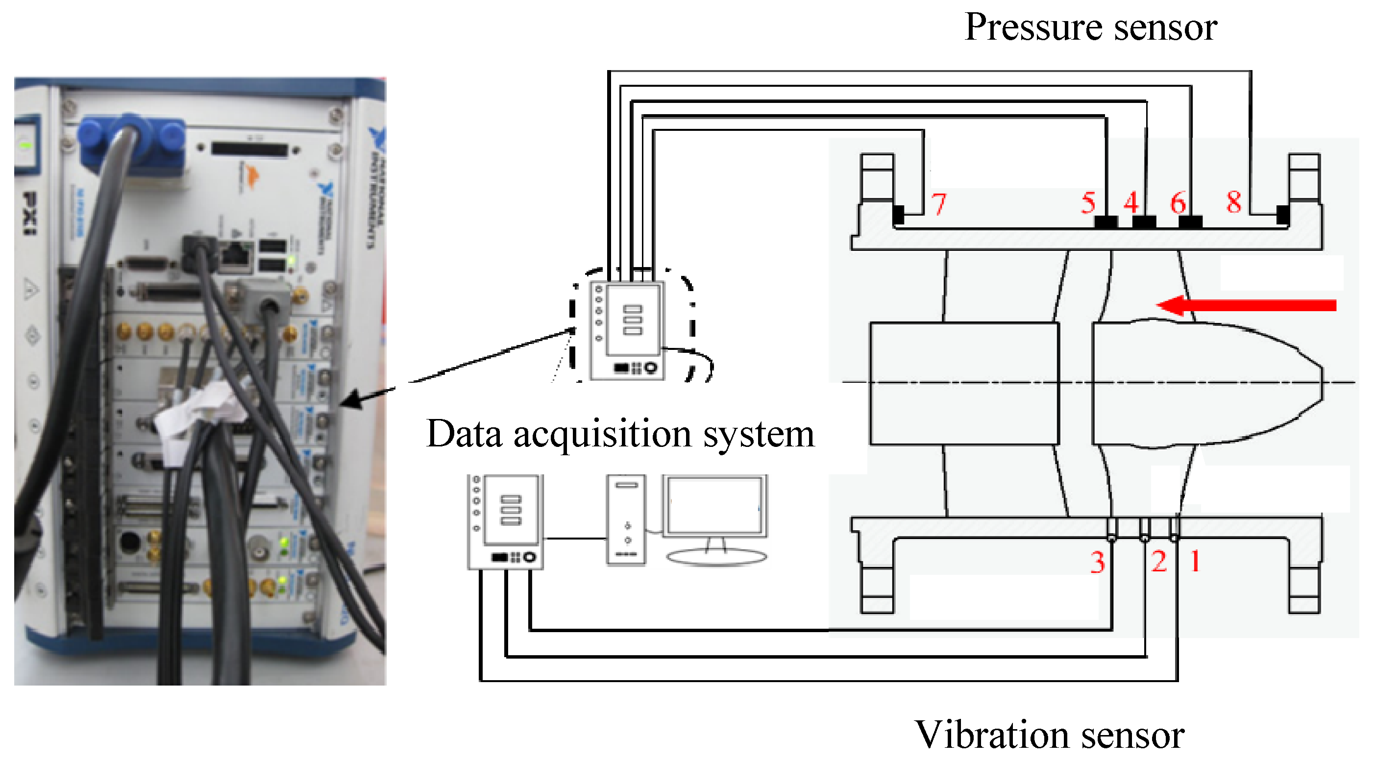
The tests on the performance and high-speed imaging of the axial flow pump were conducted at the closed test facility shown in Figure 4. The test setup included a water tank, vapor erosion tank, vacuum pump, inlet and outlet gate valves, inlet piping, motor, torque meter, model pump test section, outlet piping, booster pump, and turbine flowmeter. Figure 5 illustrates the high-speed photography experimental system, which employs a fully transparent plexiglass runner chamber to enable clear visualization of the impeller flow field for experimental imaging. The high-speed camera used for the experiments is the i-speed3, with a sampling frequency of 4000 Hz to achieve clearer images. The pressure pulsation and vibration measurement experiments are conducted using a stainless-steel impeller runner chamber. The layout of pressure pulsation and vibration sensors is shown in Figure 6. Transient pressure measurements were conducted using piezoelectric PCB 113B28 high-frequency pressure sensors (manufactured by PCB Piezotronics, Inc., New York, NY, USA), with 1, 2, and 3 corresponding to monitoring points P1, P2, and P3. Pressure sensors are installed by drilling pressure measurement holes on the runner chamber. The measurement range of the sensors is 0.69–690 kPa, with a sensitivity of 14.5 mV/kPa. The vibration acceleration sensors used are PCB 356A17 high-frequency vibration sensors (manufactured by PCB Piezotronics, Inc., New York, NY, USA), with a measurement range and sensitivity of 51 mV/(mm∙s−1). They were placed at positions 4–8, as shown in the diagram. The PXI data acquisition system and LabVIEW platform from National Instruments (NI) in the USA are used to experimentally measure signals such as pressure pulsations and vibrations under different flow rates and cavitation conditions.
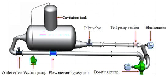
Figure 4.
The 3D schematic diagram of the axial flow pump test loop.
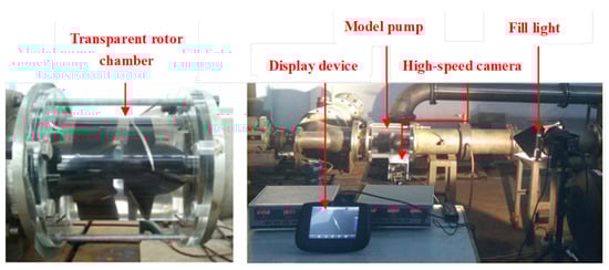
Figure 5.
High-speed camera system.
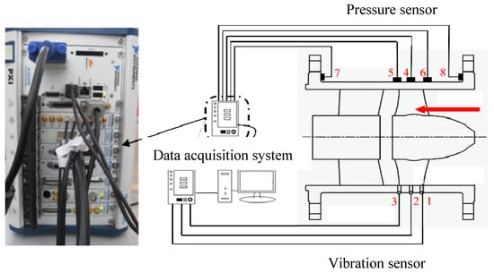
Figure 6.
Transient pressure and vibration signal data acquisition system.
2.6.2. Experimental Methods
In this paper, the active cavitation method is employed to induce cavitation in the test pump. Firstly, water is injected into the system to an appropriate level. Secondly, the air in the inlet and outlet pressure transmitters is expelled and the pressure transmitters are adjusted to the same horizontal height to eliminate the position difference. Thirdly, the coupling connecting bolts are removed, the motor is run at no load, and the torque is set to zero. Following that, the booster pump gets cranked up and the flow valve is tweaked to the testing flow rate. Once the pressure sensors at the inlet and outlet reach a steady state, the pressure readings, torque, and any other pertinent metrics are meticulously documented. For the performance tests, the flow valve is adjusted to different flow conditions and, after stabilization, the parameters for each flow rate are recorded. In conducting cavitation studies at different flow rates, the previously described procedures should be repeated. Once the system is up and running smoothly, the valve that links to the atmosphere gets sealed shut and the vacuum pump is turned on to suck the air out of the water storage tank, thereby lowering the pump’s inlet pressure. The pressure readings on the pump’s gauge are documented, and a high-speed camera session is initiated at the same time. The experiment is repeated multiple times to ensure the accuracy of the measurements. After the experiment ends, curves for the external characteristics and cavitation characteristics are plotted.
The acquisition process of transient pressure signals and vibration signals is similar to that of high-speed photography experiments. Firstly, adjust the motor speed to 1450 r/min and let the model pump run for a period of time to expel air bubbles in the water. Then, adjust the outlet flow valve to set the flowmeter to the desired flow rate. Subsequently, after the system stabilizes, close the valve connecting to the atmosphere. Initiate the vacuum suction and empty the water reservoir to lower the pump’s intake pressure, which in turn can cause cavitation in the radial flow pump. Utilize the pressure gauges to gather real-time pressure and vibration data, aligning these readings with the high-speed camera footage at various cavitation levels and pressure points. To ensure the accuracy of the experimental data, the aforementioned procedures should be repeated for various flow rates and cavitation conditions.
Experimental results were obtained by systematically measuring key performance metrics—flow rate (Q), head (H), and torque (T)—at the designated design flow rate. The total error results are as follows: flow rate (Q) = 364.4 ± 1.17 m3/h, head (H) = 3.09 ± 0.04 m, torque (T) = 232.62 ± 1.42 N·m. The turbine flowmeter employed in the study had a measurement accuracy of 0.2%, while the pressure transducer maintained precision within ±1% of the recorded values.
2.7. Analysis of Experimental Results
The performance curves obtained through experiments can also be used to verify the accuracy of numerical simulations, as shown in Figure 7, which depicts the external characteristic curves under standard atmospheric pressure, where the flow coefficient Φ in the figure is defined as
The flowrate coefficient Φ increases sequentially from 0.21 to 0.63. The corresponding flow conditions are Q/Qopt, ranging from 0.4 to 1.2 with a interval of 0.1 Qopt. The data reveals a clear alignment between the numerical predictions and experimental findings. The numerical and experimental results reveal a distinct saddle region in the performance curve of the model pump. The inflection point entering this saddle region occurs near the flowrate coefficient of Φ = 0.42. Prior to this point, the head increases with decreasing flow rate. Upon entering the saddle region, the head demonstrates a declining trend until reaching Φ = 0.32–0.38. This flow range corresponds to deep stall conditions, where complex transient flow phenomena occur within the pump. The interaction among tip leakage vortices, stall vortices, and cavitation vortices leads to discrepancies between the numerically predicted minimum point in the saddle region and experimental measurements. Notably, the head coefficient exhibits an inverse relationship with flow rate, gradually increasing as the throughput diminishes. When Φ is less than 0.37, the experimental values are greater than the numerical calculation results. When Φ is greater than 0.37, the numerical calculation results are greater than the experimental values, with a maximum error between the numerical calculation results and the experimental results of 3.8%. The head-efficiency curve exhibits a parabolic form, with efficiency first increasing and then decreasing as the flow coefficient decreases. The optimal efficiency point occurs at rated conditions, with a maximum error in efficiency of 3.6%.
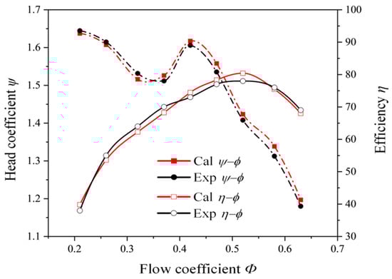
Figure 7.
Performance curves of the test pump.
Figure 7.
Performance curves of the test pump.
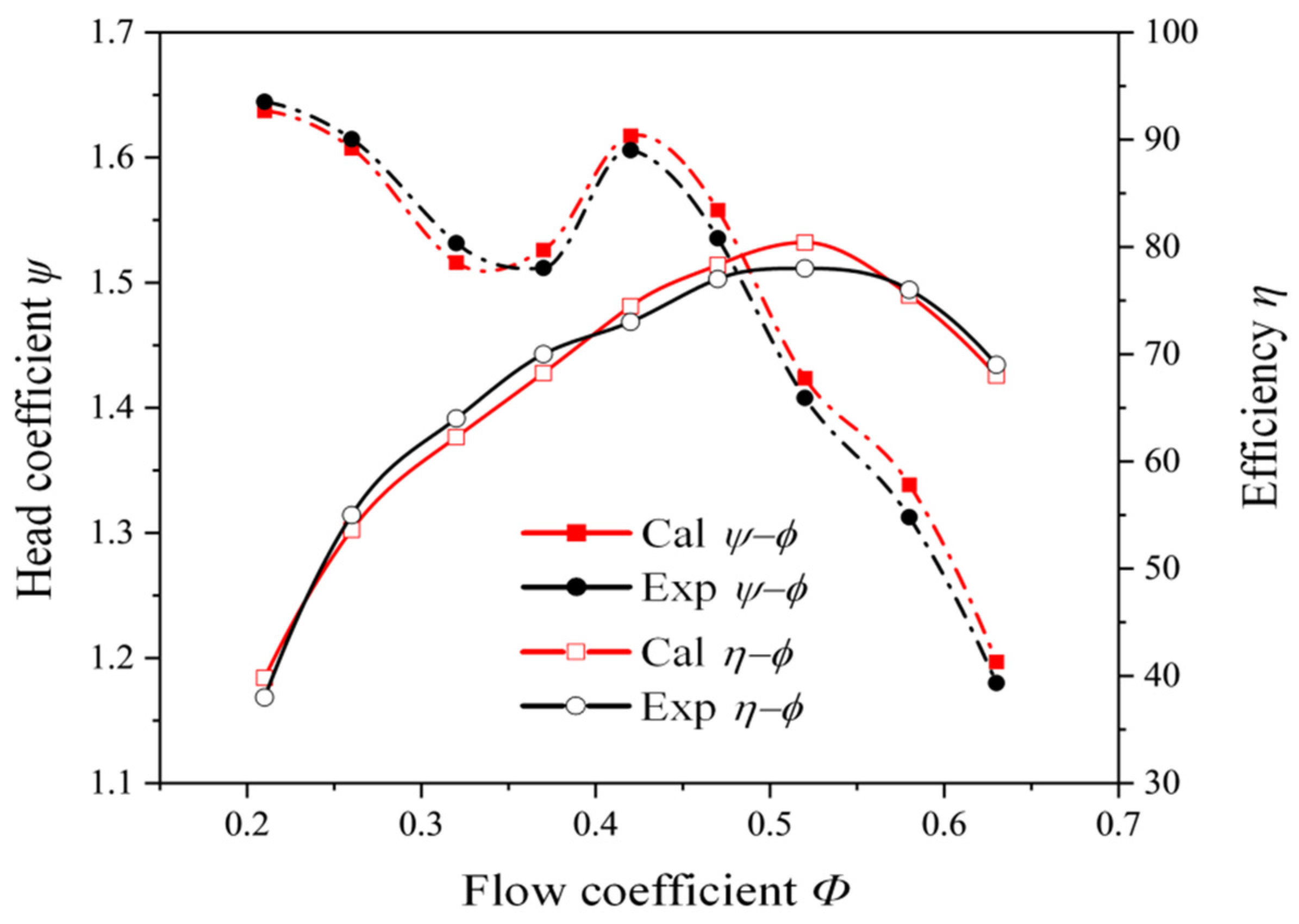
The cavitation number σ of the pump is defined as
where Pin represents the inlet pressure, Pa; Pva represents the saturated vapor pressure, Pa; ρ represents the fluid density, kg/m3; and u2 represents the linear velocity at the circumference of the impeller tip, m/s.
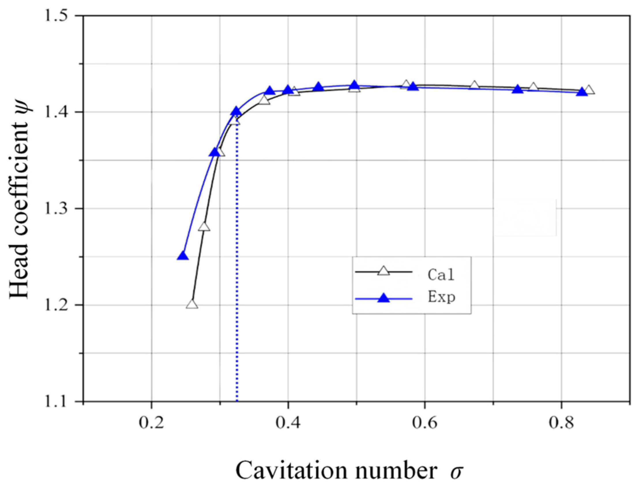
The flow coefficient Φ values corresponding to Q/Qopt = 1.2, 1.0, and 0.8 are 0.63, 0.52, and 0.42. Figure 8 displays the cavitation performance curve under normal operating conditions (Φ = 0.52). The graph reveals that as the cavitation number drops, the head coefficient experiences a modest rise. This occurs because, during cavitation’s early phases, a limited number of bubbles form on the blade surfaces. These bubbles cling to the blades, effectively creating a smoother surface that enhances performance. The friction resistance between the fluid and the smooth blade surface decreases, resulting in reduced losses. As the inlet pressure continues to drop, cavitation bubbles multiply across the blade surface and near the tip. These bubbles disrupt the flow, creating turbulence that throws the system into chaos. The resulting instability degrades the pump’s head performance and reduces the blade’s efficiency in energy transfer. When the cavitation number falls below a critical threshold, the head on the cavitation curve drops sharply, exhibiting a steep gradient. This critical point is defined as the critical cavitation number σc at the current flow rate, with a common criterion of a 3% decrease in pump head used to define the cavitation critical point. A lower cavitation number correlates with a more pronounced decrease in head and a sharper slope, resulting in a more substantial reduction in pump efficiency. Analysis of the results obtained from numerical calculations and experiments shows that the maximum error does not exceed 5%, indicating that the simulations presented in this paper are relatively accurate.
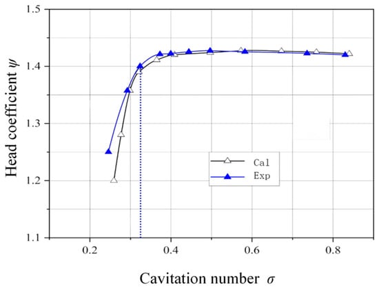
Figure 8.
The cavitation performance curves of Φ = 0.52.
3. Results and Discussion
3.1. Tip Cavitation Patterns Under Varying Flow States
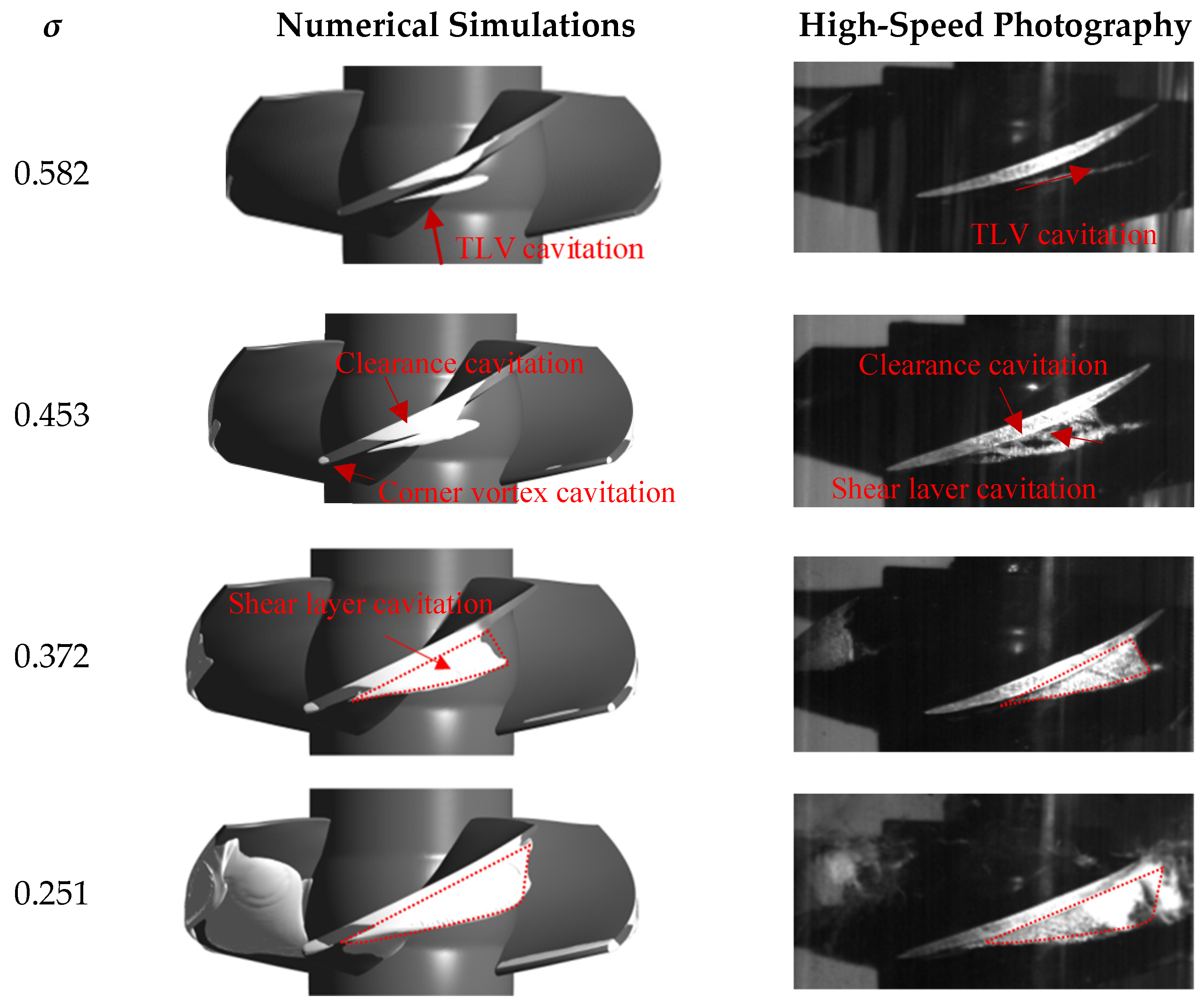
The intricate cavitation phenomena near the blade tip disrupt the primary flow, leading to partial flow obstruction and diminished pump efficiency. To visualize the tip cavitation at four distinct cavitation conditions, we employed both numerical models and high-speed photography. Figure 9 illustrates the cavitation morphology at the tip of the blade of an axial pump as a direct outcome of these methods, recorded under the operating condition of design flow rate Φ = 0.52.

Figure 9.
Cavitation pattern outcomes at Φ = 0.52 (vapor volume fraction αv = 0.1).
In the blade-tip region, numerical simulations of cavitation morphology align nicely with experimental findings, particularly at identical cavitation numbers. Notably, the blade tip’s cavitation structure undergoes considerable transformation as the cavitation number varies. To furnish a quantitative description of cavitation–cloud evolution, this study introduces a cavitation-area coefficient s*.
where scav represents the projected area of the cavitating cloud, mm2; and sframe represents the area of view captured within a single high-speed photography frame, mm2.
At a cavitation number of σ = 0.582, elongated TLV cavitation and tip vortex cavitation are observed in the blade-tip region, with a cavitation-area coefficient s* = 5.2%. Contrastingly, the flow passage exhibits no major cavitation activity. The cavitation’s influence on the pump’s overall performance is rather minimal. When the cavitation number is reduced to σ = 0.453, the cavitation-area coefficient s* increases to 11.4% and pronounced corner vortex cavitation emerges at the leading-edge corner between the blade tip and the end-wall. The tip vortex cavitation further develops and interacts with TLV cavitation, forming a shear-layer cavitation structure. When σ = 0.372, corner vortex cavitation intensifies markedly, and the cavitation-area coefficient s* rises to 13.6%. The tip vortex cavitation extends along the chord length of the blade. At this point, the cavitation structure evolves into a triangular cavitation structure consisting of TLV cavitation, tip vortex cavitation, and shear layer cavitation. Additionally, attached sheet cavitation also occurs on the suction surface of the blade. When σ = 0.251, the cavitation-area coefficient s* reaches 16.9%, with the triangular cavitation cloud spanning nearly the entire blade-tip region and unsteady shedding vortex cavitation forming at the blade trailing edge. The area of attached sheet cavitation on the blade’s suction surface continues to expand. The extensive cavitation on the blade surface and the tip cavitation cloud interact with the mainstream, resulting in an unsteady flow field. The extensive cavitation impedes the flow, thereby reducing the impeller’s operational efficiency and significantly degrading the pump’s performance. The high-speed photography is a reasonable and accurate method for determining the cavitation inception point. However, due to its high requirements for the test object and test environment, it is only suitable for limited applications. To effectively analyze how signal patterns shift across various cavitation phases, we categorize the cavitation intensity into four distinct levels: standard operation, slight cavitation, intermediate cavitation, and extreme cavitation. This classification is derived from high-speed imagery and bolstered by numerical simulations. Figure 10 presents the cavitation coefficients associated with these four operational states at varying flow rates.
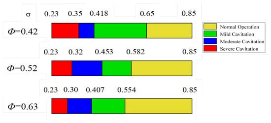
Figure 10.
Classification of different cavitation levels.
3.2. Evolution of Tip Cavitation of an Axial Flow Pump
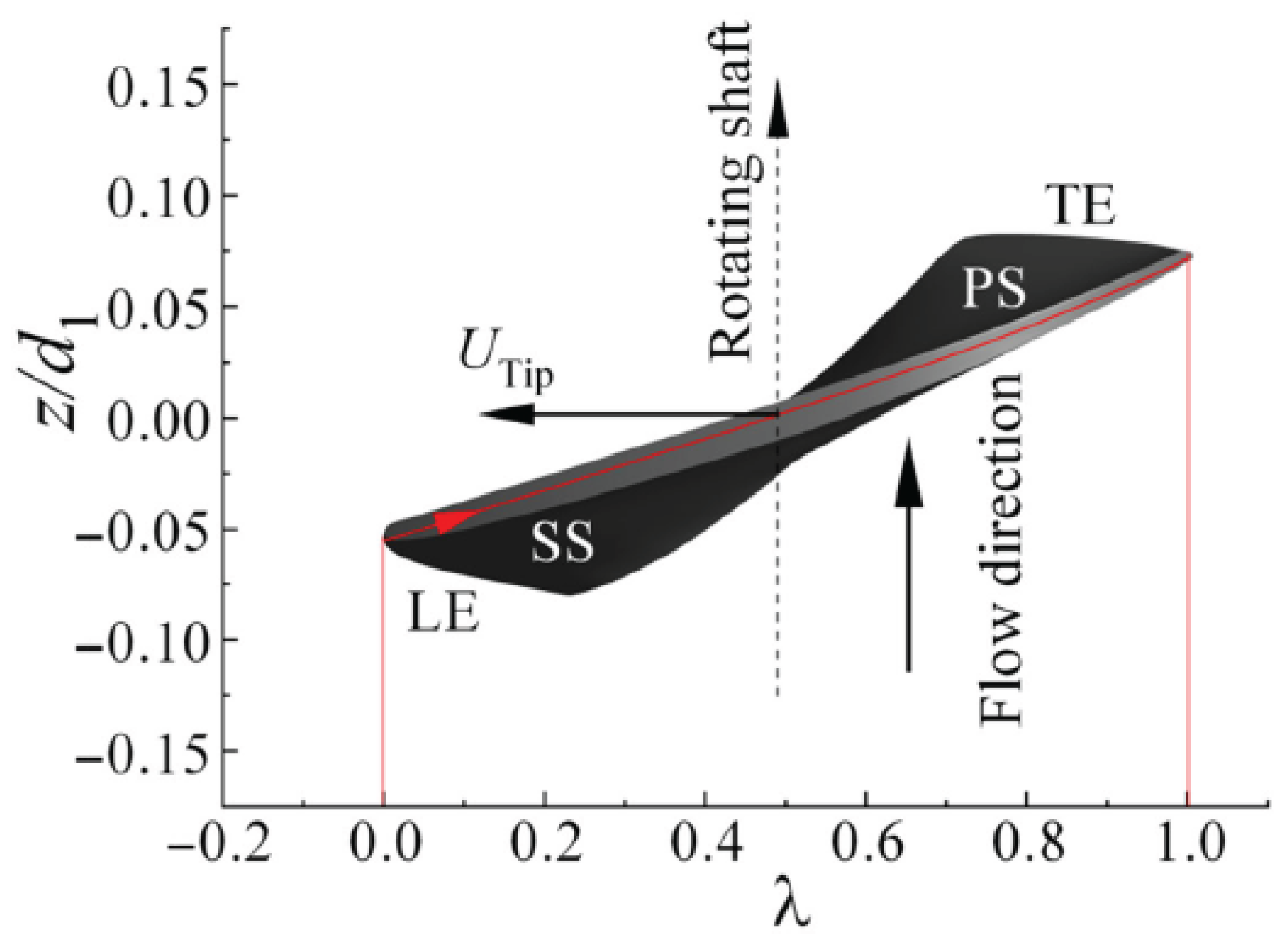
During severe cavitation, a large triangular cavitation cloud becomes evident at the tip of the impeller blade. To delve into the fleeting cavitation traits exhibited by the blade tip’s morphological cavitation during the intense cavitation phase under various flow conditions, this study introduces the blade chord length ratio λ, as depicted in Figure 11.
where l refers to the length from the outer margin of the blade’s leading edge to the axis of the blade at each chord’s transverse section, mm; and c represents the total length from the blade’s leading edge to its trailing edge, mm.
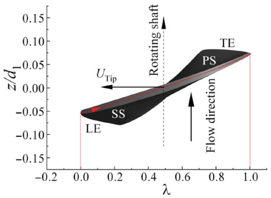
Figure 11.
Definition of the blade chord coefficient λ.
Both Figure 12 and Figure 13 are results captured from high-speed photography experiments. Figure 12 shows the transient evolution of cavitation in the tip region at a lower cavitation number, spanning from 0 ms to 4 ms. The red dashed lines in the figure correspond to different chord length coefficients. From Figure 12a, it can be seen that in the flow condition of Φ = 0.42, the cavitating structures within the tip region consist of TLV, clearance, and shear layer cavitation, which coalesce into a large triangular cloud. The trailing edge of the cavitation cloud is originally located at λ = 0.7. Within the λ range of 0.5 to 0.7, unstable vortex cavitation constitutes the cavitation phenomenon. As the impeller rotates, the unstable vortex structures at the trailing edge of the cavitation cloud dissipate and detach, forming a vertical cavitation vortex (SSPCV) perpendicular to the suction surface of the blade at t = 2 ms. Under design conditions (Φ = 0.52), the tip cavitation cloud initially forms at λ = 0.1 and remains stably attached between λ = 0.1 and λ = 0.7. The cavitation morphology and coverage exhibit minimal temporal variation across different instantaneous time frames. However, two oscillating cavitation wakes are observed downstream of the primary cavitation cloud. These wake structures demonstrate continuous shape modulation while maintaining coherent attachment to the trailing edge of the primary cavitation cloud without detachment. The triangular cavitation cloud is notably smaller than that depicted in Figure 12a, and the tip leakage vortex forms a smaller angle with the blade chord. Under high-flow conditions (Φ = 0.63), the tip leakage vortex originates at the blade chord length coefficient λ = 0.5. The cavitation pattern primarily consists of tip-leakage vortex cavitation and clearance cavitation, with cloud cavitation being less pronounced. At distinct instantaneous time points, the scale and intensity of the cavitation vortex structure associated with the tip leakage vortex show minimal variation. This observation indicates that under low-flow conditions, the unstable flow phenomena within the pump enhance the transient characteristics of cavitation in the tip region.
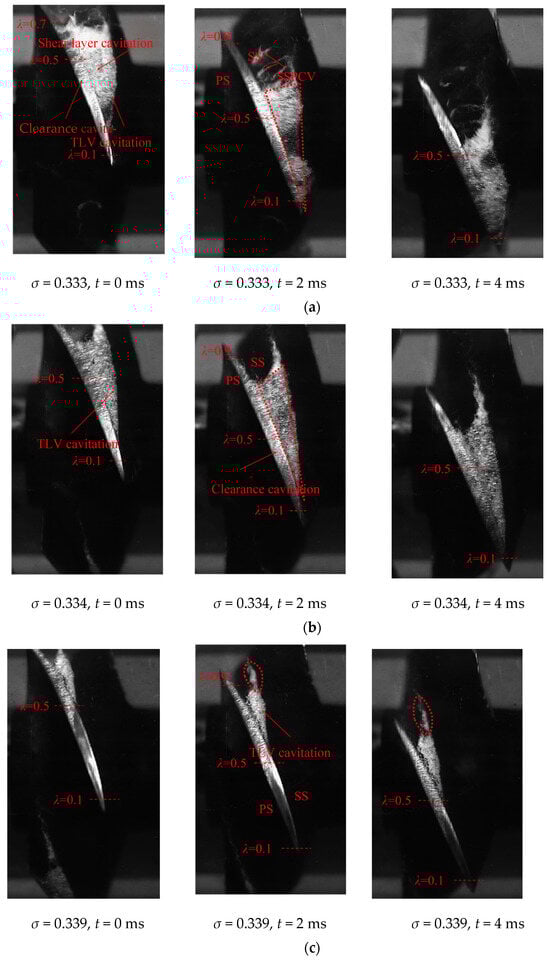
Figure 12.
Transient cavitation patterns of lower cavitation numbers at different flow rates: (a) Φ = 0.42; (b) Φ = 0.52; (c) Φ = 0.63.

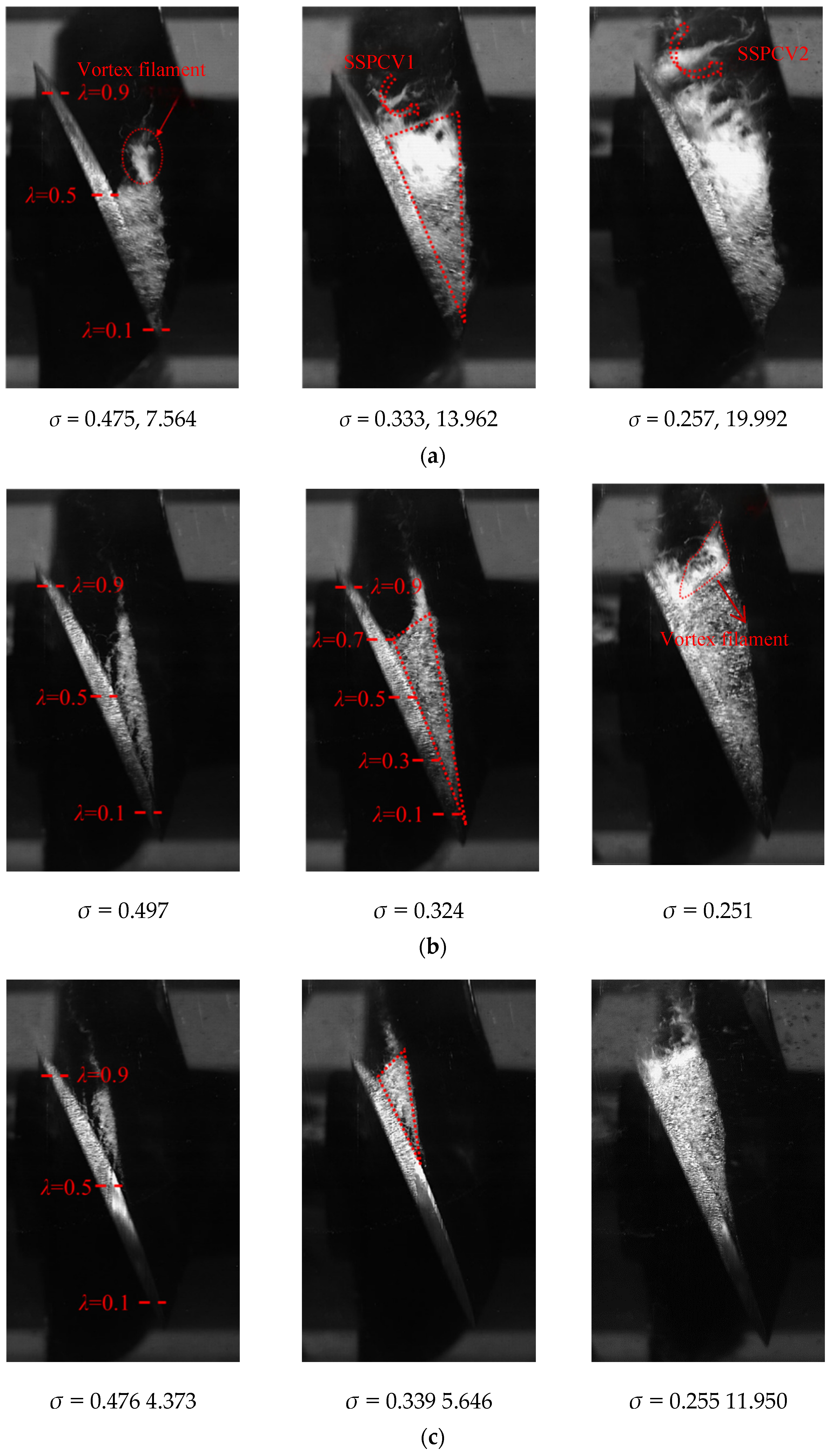
Figure 13.
Cavitation patterns for different cavitation numbers at different flowrates: (a) Φ = 0.42; (b) Φ = 0.52; (c) Φ = 0.63.
Cavitation in axial flow pumps leads to a decrease in pump performance and causes significant flow losses. Figure 13 illustrates cavitation formations at the blade tip across various cavitation numbers, corresponding to flow rates of Φ = 0.42, Φ = 0.52, and Φ = 0.63. When operating at the designed flow rate with a cavitation number of σ = 0.497, the only forms of cavitation observed are elongated tip-leakage vortex (TLV) cavitation and clearance cavitation, and the cavitation-area coefficient s* is 6.3%. These phenomena are confined to the blade’s tip region and occur specifically within a chord length coefficient range of λ = 0.1 to 0.5. At this stage, the effect on the pump’s efficiency remains minimal. However, once the cavitation number drops to 0.324, the cavitation area expands to reach λ = 0.7 and the cavitation-area coefficient s* is reduced to 5.1%, effectively enveloping the blade-tip region with a triangular array of cavitation clouds. As the cavitation number drops, the cavitation reaches the blade’s trailing edge, creating slender vortex filaments along the cavitation structure’s trailing perimeter. At Φ = 0.42, as depicted on the curve of cavitation characteristics, cavitation propensity increases at reduced flow rates under consistent operational parameters. At a cavitation number of σ = 0.475, a complex cavitation cloud emerges near the blade tip, corresponding to the cavitation-area coefficient s* = 7.6%. This structure originates from the synergistic coupling among shear layer cavitation, clearance cavitation, and tip-leakage vortex (TLV) cavitation. Additionally, when λ reaches 0.5, slender vortex filament structures develop along the trailing edge of the cavitation zone. As cavitation intensifies, SSPCVs can be observed. When the cavitation number σ = 0.333, SSPCV1 detaches from λ = 0.7 and rapidly dissipates in the flow passage and the cavitation-area coefficient s* is 14.1%. When the cavitation number σ = 0.257, the size and intensity of the SSPCVs increase, the cavitation-area coefficient s* rises to 20.1%, and its initial formation position shifts towards the trailing edge of the blade along with the extent of the triangular cloud cavitation. As the impeller rotates, the SSPCV2 gradually extends into the flow passage until it is severed by an adjacent blade. Its obstruction of the flow passage leads to a decline in the performance of the experimental pump. At Φ = 0.63 and σ = 0.476, compared to the design flow rate with the same cavitation number, TLV cavitation occurs at λ = 0.5. This occurs because at high flow velocities, changes in the flow angle cause the cavitation inception point to shift rearward. When the cavitation becomes extremely intense, the affected area at the blade tip extends across the entire blade tip once λ reaches 0.5.
3.3. Experimental Analysis of Cavitation-Induced Tip Pressure Fluctuations in Axial Flow Pumps
When cavitation occurs in axial flow pumps, the unstable cavitating flow in the internal flow field induces unsteady pressure fluctuations within the pump, which have a significant impact on the stable operation of the pump. As shown in Figure 6, monitoring points P1, P2, and P3 are set near the tip of the flow passage to investigate the pressure fluctuations caused by cavitation in the impeller of the axial flow pump. Given the extreme pressure levels inside the impeller during pump operation and the effect of static pressure readings at the monitoring points, we need a clear way to assess how cavitation influences transient pressure near the blade tips. To achieve this, the experimental data from the monitoring points is normalized. The pressure fluctuation coefficient, denoted as Cp, is calculated using the following formula:
where p represents the instantaneous pressure at the monitoring location, Pa; and ρ represents the fluid’s density, kg/m3.
3.3.1. Characteristics of Pressure Fluctuations Under Different Cavitation Conditions
To examine how different cavitation conditions influence pressure fluctuations near the blade tip of an axial flow pump, researchers processed the pressure data by averaging it over time and converting it into dimensionless form. This approach yielded clear time-domain representations for comparison. Frequency-domain information was processed and analyzed using the Fast Fourier Transform (FFT). The model pump in this investigation operates at an impeller rotation speed n = 1450 rpm. Converting this rotational speed to shaft frequency yields fz = n/60 = 24.17 Hz. Furthermore, the blade frequency fn is calculated as four times the shaft frequency (since there are four blades), resulting in fn = 96.7 Hz. The blade multiple N is defined as the ratio of the frequency to the blade frequency:
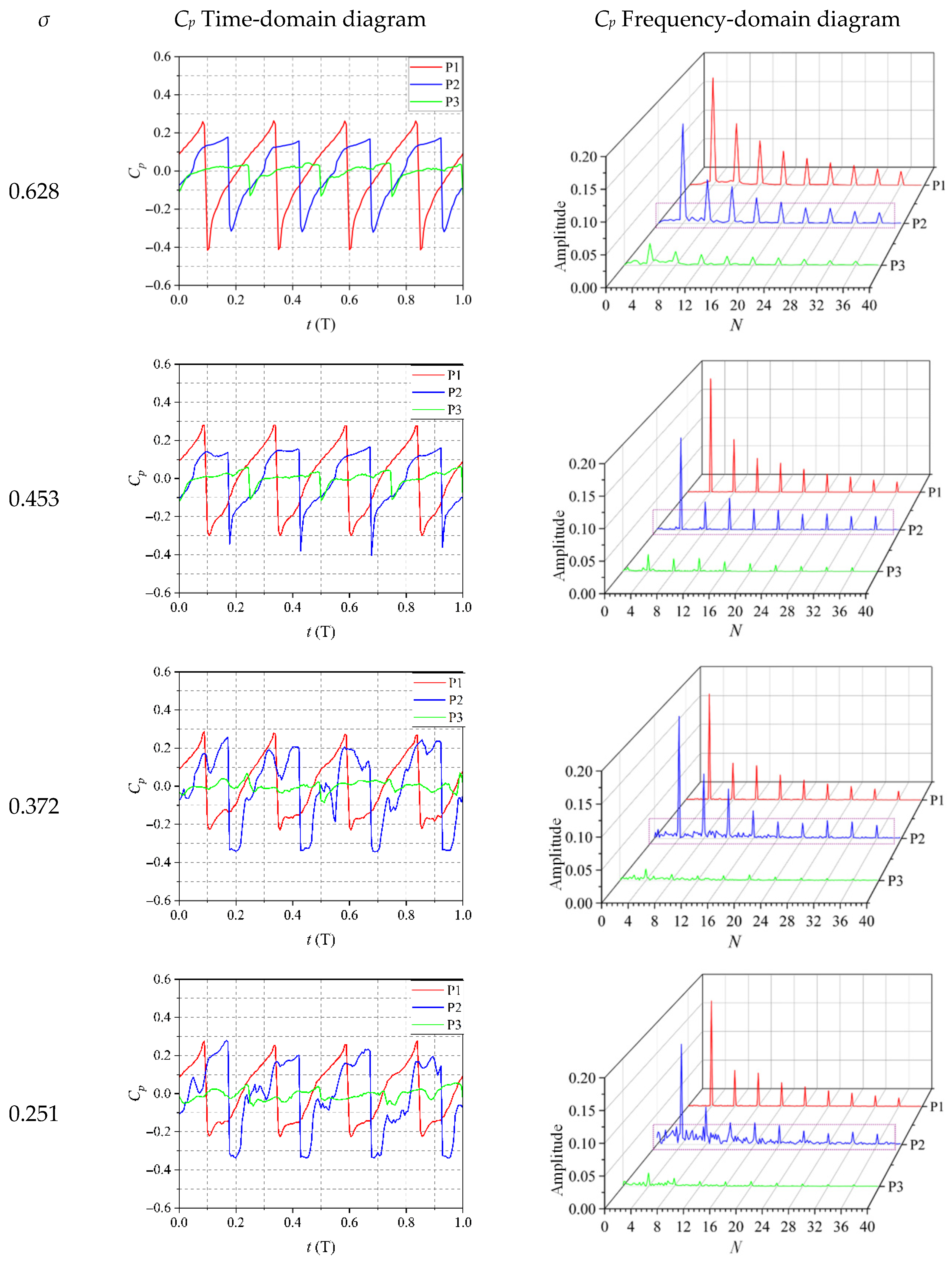
By analyzing the transient pressure fluctuations in the tip region under different cavitation numbers, in Figure 14, we can observe the time- and frequency-domain representations of pressure variations at points P1, P2, and P3 over a single cycle T. These plots depict the results of numerical simulations conducted under four distinct cavitation scenarios, all with the flowrate coefficient of Φ = 0.52. Within one period T, four peaks and troughs corresponding to the number of blades are observed. This shows the impeller produces consistent pressure variations at the blade tip during normal operation. By comparing the time-domain plots of various monitoring points under different cavitation numbers, as the cavitation number decreases, significant secondary pressure fluctuations appear in the 1/4 T period from the suction side to the pressure side at the monitoring points in the tip region. This suggests that the pressure fluctuations in the tip region are significantly affected by cavitation during the recovery of the pressure coefficient. The influence of fluctuation characteristics becomes more pronounced at lower cavitation numbers. By comparing the frequency-domain plots of pressure fluctuations at different monitoring points, the blade frequency corresponding to each monitoring point is the dominant frequency with the maximum amplitude. At monitoring point P2, as indicated by the purple dashed box in the frequency-domain plot, as the cavitation number decreases, the complexity of cavitation in the blade-tip region increases. As the impeller moves beyond P2, cavitation influences its operation, generating prominent low-frequency signals under one blade frequency. High-frequency components also appear within the range from one to three times the blade frequency and above three times the blade frequency. Moreover, as the cavitation number decreases, the amplitudes of both the high-frequency and low-frequency components increase. This indicates that at lower cavitation numbers, the intensity of cavitation and the impact of unstable cavity collapse on the blade-tip region become stronger. Therefore, the pressure fluctuations at monitoring point P2 are more significantly affected by the severity of cavitation.
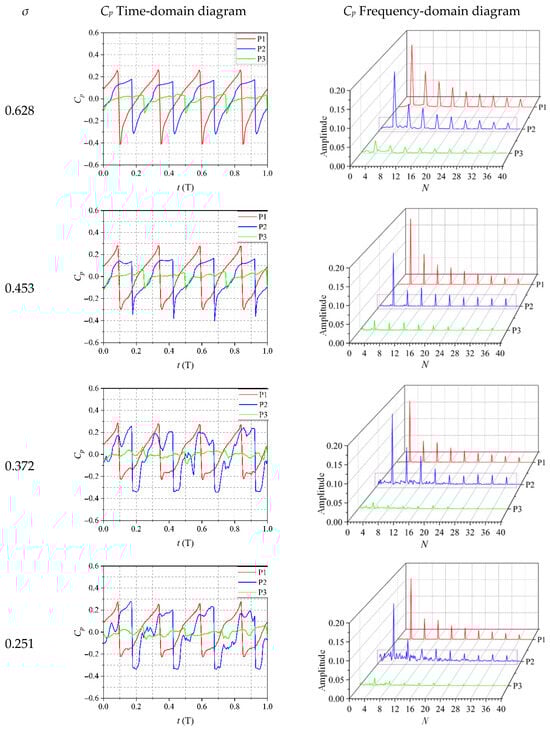
Figure 14.
Pressure fluctuation signal characteristics at the monitoring point (time and frequency domains).
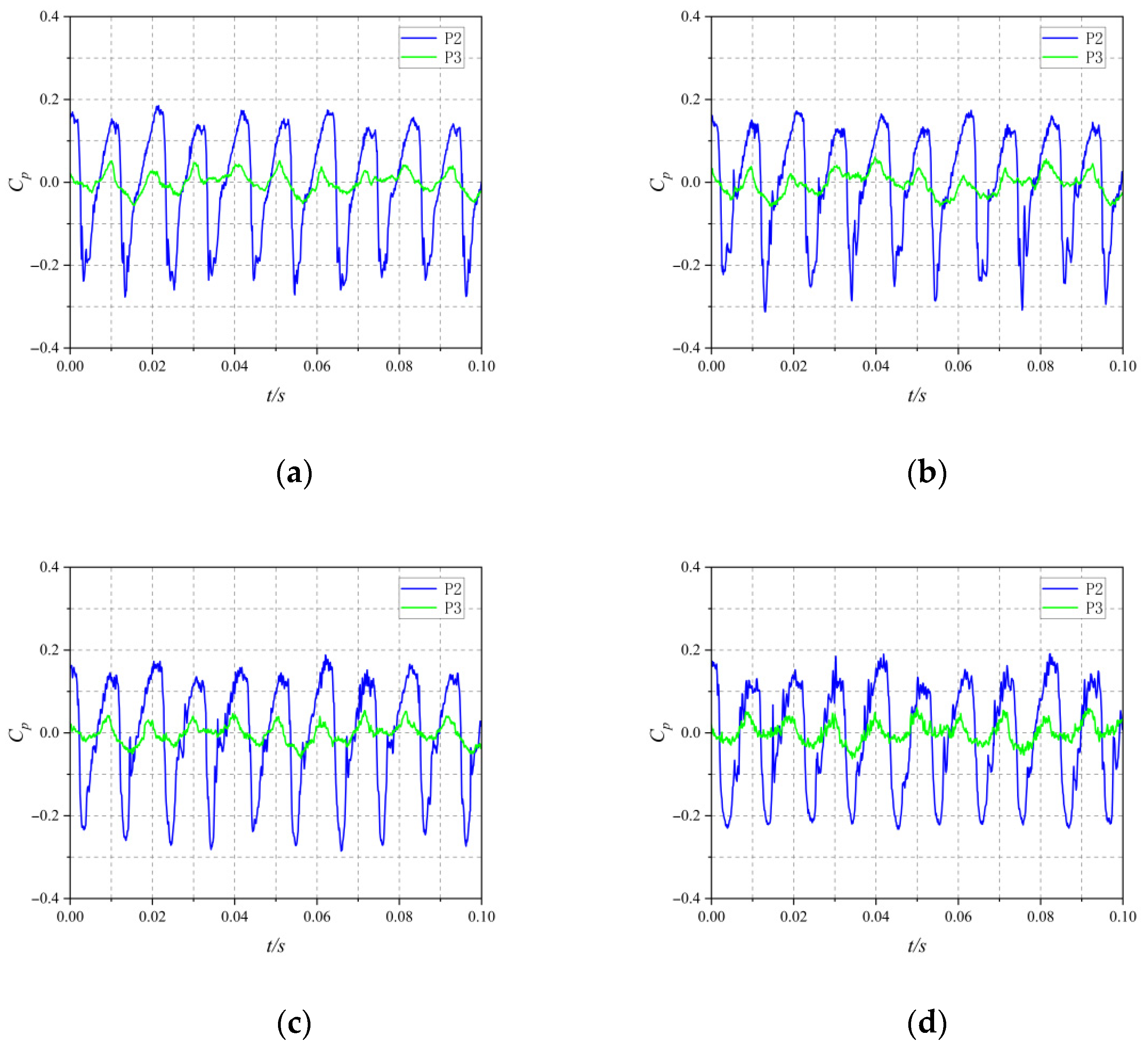
Based on pressure fluctuation measurements, the experimental monitoring points P2 and P3 are selected for analysis. Four cavitation cases at Φ = 0.52 are analyzed, with σ values of 0.497, 0.399, 0.324, and 0.246. Comparative analysis is conducted on the pressure fluctuation monitoring points P2 and P3. Figure 15 shows relatively consistent pressure fluctuation patterns within the impeller. There is a temporal offset between the peaks and troughs of the experimental monitoring points P2 and P3. This is attributed to the pressure fluctuation sensors being installed parallel to the rotational axis, such that the impeller inlet first passes through monitoring point P2 before reaching monitoring point P3. At monitoring location P2, the blade tip’s excessive gap has led to a substantial secondary surge, which shows up as the blade moves from its pressure side to the suction side. As the flow shifts from the suction surface toward the pressure surface, secondary fluctuations emerge in the pressure coefficient’s recovery phase on the waveform diagram. This occurs because of the interplay between tip-leakage vortex cavitation and shear layer cavitation, which disrupts the smooth pressure transition. Furthermore, as the cavitation number decreases, the frequency of secondary fluctuations increases during the recovery from the trough to the peak. This is because when the cavitation number is low, the area of the triangular cavitation cloud region at the blade tip increases, and the intensities of tip clearance cavitation, TLV cavitation, and shear layer cavitation increase, resulting in more secondary fluctuations during the recovery of the pressure coefficient at monitoring point P2.
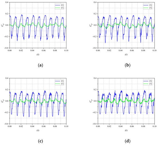
Figure 15.
Time domain of pressure fluctuation signal at Φ = 0.52: (a) σ = 0.497; (b) σ = 0.399; (c) σ = 0.324; (d) σ = 0.246.
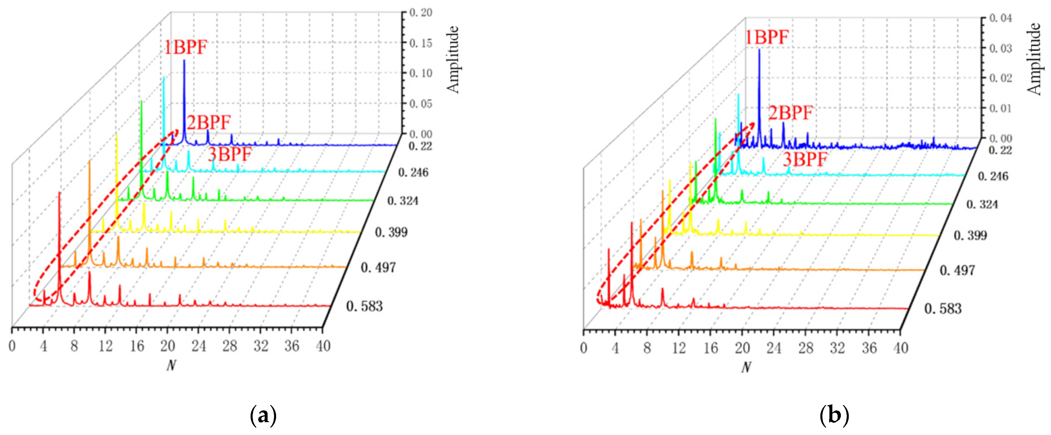
As shown in Figure 16, the frequency-domain distributions of pressure fluctuations under the design condition are presented. The dominant frequencies at monitoring points P2 and P3 are the blade passing frequency (BPF) and its harmonics. Under varying cavitation conditions, a low-frequency component with N = 3 is observed at monitoring point P2. At monitoring point P3, low-frequency components with N = 1 and N = 3 are detected. As the cavitation number drops to σ = 0.221, high-frequency signals at P3 intensify. This is because at lower cavitation numbers, the cavitation area at the blade tip increases. Monitoring point P3 is positioned at the impeller outlet’s trailing edge, where cavitation patterns are prone to instability. At monitoring point P3, N = 1 corresponds to a shaft frequency of 1450 rpm, which is associated with the impeller rotation. This indicates that, besides the dominant impeller frequency, this monitoring point is also significantly influenced by the shaft frequency. Since monitoring point P3 is situated at the impeller outlet’s trailing edge, its frequency domain traits are significantly shaped by the shaft’s rotational frequency. Additionally, the amplitude variations in the frequency domain are relatively small. Therefore, monitoring point P2 is selected for further signal analysis in the following sections.
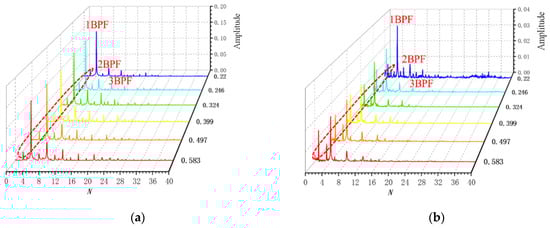
Figure 16.
Frequency domain of pressure fluctuation signal at Φ = 0.52: (a) P2 Time-domain diagram; (b) P3 Frequency-domain diagram (different colors correspond to different cavitation number conditions).
3.3.2. Characteristics of Pressure Fluctuations Under Different Flowdate Conditions
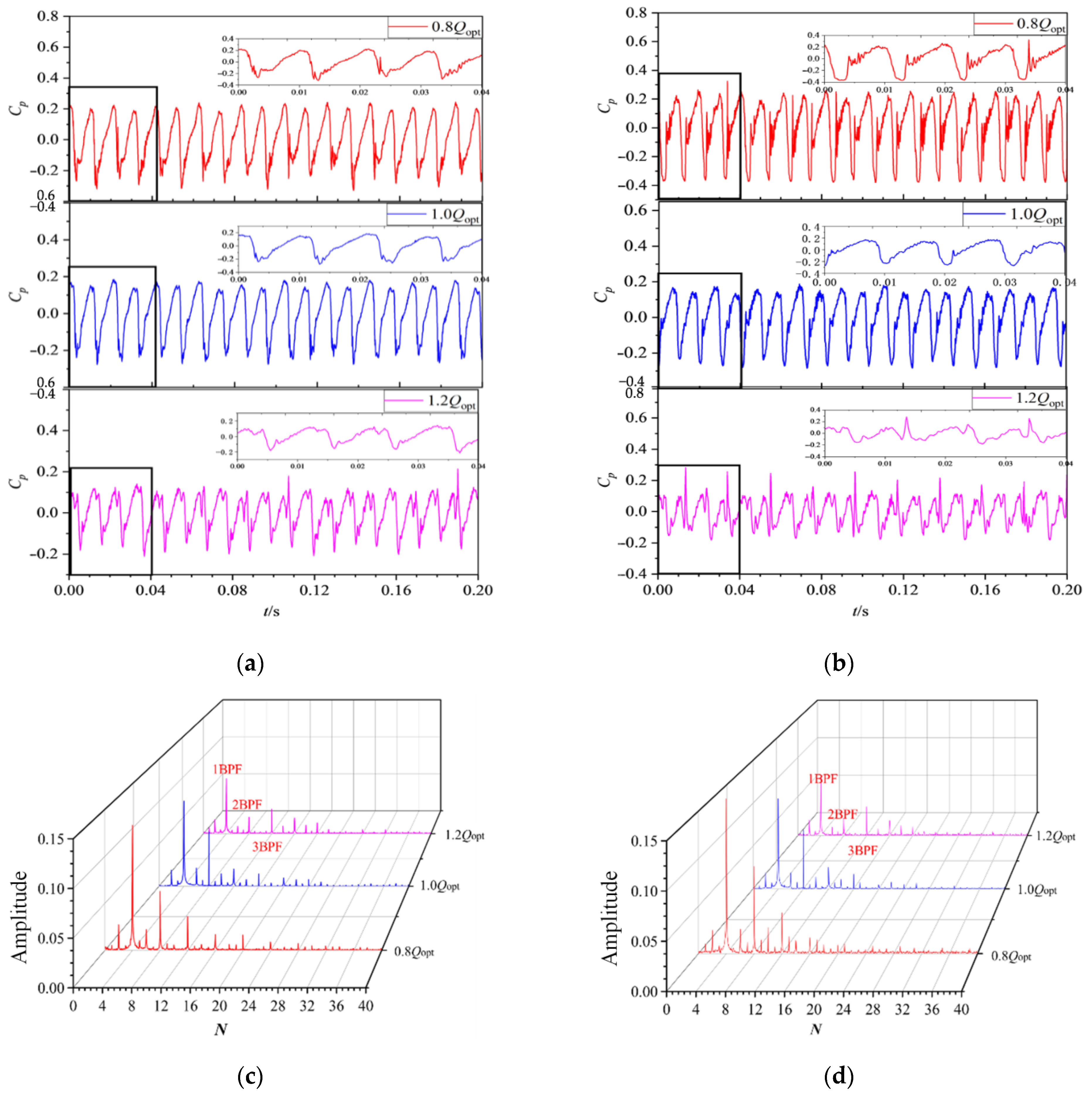
As shown in Figure 17, the time-domain and frequency-domain plots of the pressure coefficient at P2 under two typical cavitation conditions are presented. The corresponding cavitation numbers are 0.399 and 0.221, respectively. Figure 17a,b show the time-domain plots under different flow rates. Figure 17c,d display the frequency-domain plots after Fast Fourier Transform (FFT). The insets in the figures capture the transient pressure behavior within one impeller revolution. As the impeller rotates, monitoring point P2 moves from the pressure side of the blade to the suction side. The transient pressure coefficient fluctuates between peaks and troughs. As the flow rate decreases, the peak-to-peak value gradually increases. The transient pressure fluctuations become more pronounced. Especially under severe cavitation conditions, during one-quarter of an impeller revolution, as the pressure coefficient rises from the suction side to the pressure side of the blade, the pressure fluctuation characteristics are even more significant. This shows that the tip area in these cavitation circumstances is affected by complex TLV cavitation and unstable SSPVC shedding and dissipation. After FFT transformation, frequency-domain analysis of monitoring point P2 is conducted. Throughout the various phases of cavitation, the primary frequencies of pressure oscillations consistently align with the blade passing frequency and its harmonic multiples. However, as the flow rate rises, the intensity of these dominant frequencies diminishes accordingly. The data indicates that with an elevated flow rate, the pressure differential across the pressure and suction sides diminishes. Therefore, the cavitation performance is better under high-flow-rate conditions via the intensity of the tip leakage flow. At the same cavitation stage, lower flow rates are associated with larger amplitudes. The frequency characteristic fluctuations of high-frequency components are more significant. Furthermore, the noise levels were observed to increase correspondingly. This indicates that the entrainment and disturbance between the cavitation morphology in the tip region and the mainstream are stronger at lower flow rates. The unstable flow field structure in the tip region is more complex.
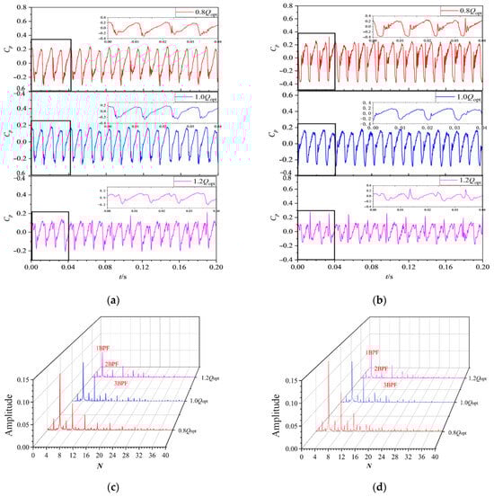
Figure 17.
Time domain and frequency domain of pressure fluctuation at P2 under different flowdate conditions: (a) σ = 0.399; (b) σ = 0.221; (c) σ = 0.399; (d) σ = 0.221.
4. Conclusions
This study employs high-speed imaging techniques and pressure fluctuation measurements alongside computational modeling to conduct a comparative examination of cavitation morphology characteristics across varying operational parameters. Four distinct cavitation levels, including normal operation, mild cavitation, moderate cavitation, and severe cavitation, were distinguished. Additionally, the evolution of impeller tip cavitation morphologies was investigated across various flow rates and cavitation numbers. Furthermore, the pressure fluctuation characteristics of cavitation in the impeller tip region were explored under different flow conditions and cavitation conditions through pressure fluctuation experiments. Compared with previous studies, this research provides detailed observations of the cavitation morphology evolving from TLV and clearance cavitation to complex triangular cavitation clouds at lower cavitation numbers. Additionally, this study found that at the same cavitation stage, lower flow rates exhibit larger pressure fluctuation amplitudes in the blade-tip region, with more significant changes in the frequency characteristics of high-frequency components. This suggests that the interaction between cavitation morphology and the mainstream is stronger at lower flow rates, leading to more complex flow structures in the tip region. These new findings provide a theoretical basis for a deeper understanding of the mechanisms of pressure fluctuations induced by cavitation in the blade-tip regions of axial flow pumps and offer references for the subsequent optimization of axial flow pump design and the mitigation of cavitation damage. The main conclusions are as follows:
- (1)
- Through a comprehensive investigation of cavitation structures at the impeller tip across different cavitation numbers, employing high-speed imaging and computational models, the results reveal satisfactory cavitation morphologies. As the cavitation number decreases and the degree of cavitation increases, the cavitation morphologies in the impeller tip region undergo complex evolution. When the cavitation number is relatively high, there are no obvious vapor bubbles in the impeller tip region. As the cavitation number diminishes, the impeller tip area exhibits TLV and clearance cavitation, yet no substantial corner vortex cavitation is produced. As the cavitation number drops further, vortex cavitation appears along the blade’s leading edge, while both tip leakage and clearance cavitation expand, eventually merging into a distinctive triangular cloud formation. Under intense cavitation conditions, vortex cavitation near the blade corners and triangular cavitation clusters along the leading edge significantly expand within the impeller tip region. This expansion coincides with a marked deterioration in the pump’s operational efficiency. Based on the occurrence and development of cavitation at different cavitation numbers, as well as the evolution characteristics of cavitation area and morphology, the severity of cavitation is classified into four states: normal operation, mild cavitation, moderate cavitation, and severe cavitation.
- (2)
- Under different cavitation conditions, the head coefficient exhibits a trend of slightly increasing initially and then decreasing sharply. When evaluating cavitation behavior across varying flow rates, partial-load operation tends to trigger cavitation more readily inside the pump, with its unsteady flow effects becoming particularly noticeable. At lower cavitation numbers, a perpendicular vertical cavitation vortex (SSPCV) develops alongside the blade’s suction face. When cavitation intensifies, the SSPCV increases in size and strength, migrating toward the trailing edge of the impeller tip as the triangular cavitation region expands. At higher flow rates, TLV cavitation begins at λ = 0.5, but as the flow diminishes, the onset point of TLV cavitation shifts upstream.
- (3)
- Numerical simulations of the transient pressure fluctuations across various operational scenarios reveal that the pressure coefficient Cp at the gauge positioned close to the blade edge undergoes considerable fluctuations over time, which are notably influenced by the differing cavitation conditions. The monitoring point P2 is significantly affected by cavitation. As the cavitation number decreases, significant low-frequency and high-frequency components appear at monitoring point P2. Furthermore, as cavitation intensifies, the amplitudes of both low-frequency and high-frequency components increase. Under the same flow rate, reducing the cavitation number transforms the blade-tip region from TLV and clearance cavitation into a triangular cavitation cloud. As the pressure coefficient increases from its trough to its peak, corresponding to the monitoring point traversing the complex cavitation structure region from the blade’s suction side to its pressure side, numerous secondary fluctuation characteristics emerge.
- (4)
- By comparing the transient pressure measurement results from different cavitation experiments, both experimental and numerical results exhibit identical pressure fluctuation characteristics. Frequency domain analysis reveals that the dominant frequencies at monitoring points P2 and P3 are both the blade passage frequency. Monitoring point P3 is more significantly influenced by the shaft frequency. Across various cavitation stages, the dominant frequencies of pressure fluctuations under different flow conditions are the impeller passage frequency and its harmonics. The amplitude of the dominant frequency decreases as the flow rate increases. When we examine the pressure fluctuation data across varying flow rates, a clear pattern emerges. It appears that at comparable stages of cavitation, lower flow rates tend to produce more pronounced pressure fluctuations. Specifically, we observe larger amplitudes and more substantial variations in the high-frequency components of the frequency spectrum. This indicates that the entrainment and disturbance between the cavitation morphology in the blade-tip region and the mainstream are stronger at lower flow rates, resulting in more complex unstable flow field structures in the blade-tip region.
Author Contributions
Conceptualization, H.W. and X.S.; Methodology, H.W.; Software, H.W.; Validation, H.W.; Formal analysis, H.W.; Investigation, H.W.; Data curation, H.W., C.N. and G.Y.; Writing—original draft, H.W.; Writing—review & editing, H.W.; Supervision, X.S. All authors have read and agreed to the published version of the manuscript.
Funding
This research was funded by the National Natural Science Foundation of China, grant numbers 52409117; the Jiangsu Province Science Foundation for Youths, grant number BK20230540; and the Natural Science Foundation of the Jiangsu Higher Education Institutions of China, grant number 23KJB570001.
Data Availability Statement
The original contributions presented in this study are included in the article. Further inquiries can be directed to the corresponding author.
Conflicts of Interest
The authors declare no conflict of interest.
Nomenclature
| Symbols | |
| D1 | Diameter of inlet pipe (m) |
| Z | Number of impeller blades |
| D2 | Diameter of impeller (m) |
| Zd | Number of diffuser blades |
| n | Design rotating speed(r/min) |
| Qopt | Design flow rate (m3/s) |
| H | Delivery head (m) |
| τ | Tip clearance (m) |
| σ | Cavitation number |
| Φ | Flowrate coefficient |
| y+ | Non-dimensional distance from the wall |
| ψ | Head coefficient of the pump |
| η | Efficiency |
| λ | Blade chord coefficient |
| Cp | Pressure fluctuation coefficient |
| ρ | Density (kg/m3) |
| N | Ratio of the frequency to the blade frequency |
| Abbreviations | |
| TLV | Tip leakage vortex |
| SSPCV | Suction-side perpendicular cavitating vortex |
References
- Luo, X.; Ji, B.; Tsujimoto, Y. A review of cavitation in hydraulic machinery. J. Hydrodyn. 2016, 28, 335–358. [Google Scholar] [CrossRef]
- Shi, W.; Li, T. Numerical simulation of tip clearance leakage vortex flow characteristic in axial flow pump. J. IOP Conf. Ser. Earth Environ. Sci. 2012, 15, 2023. [Google Scholar] [CrossRef]
- Shen, J.; Hong, Y. Effect of tip clearance on unsteady flow in axial-flow pump. J. Drain. Irrig. Mach. Eng. 2013, 31, 667–673. [Google Scholar]
- Gopalan, S.; Katz, J. Effect of Gap Size on Tip Leakage Cavitation Inception, Associated Noise and Flow Structure. J. Fluids Eng. 2002, 124, 994–1004. [Google Scholar] [CrossRef]
- Pouffary, B.; Patella, R. Numerical Simulation of 3D Cavitating Flows: Analysis of Cavitation Head Drop in Turbomachinery. J. Fluids Eng. 2008, 130, 061301. [Google Scholar] [CrossRef]
- Chen, H.; Li, J. Thermal Effect at the Incipient Stage of Cavitation Erosion on a Stainless Steel in Ultrasonic Vibration Cavitation. J. Fluids Eng. 2009, 131, 024501. [Google Scholar] [CrossRef]
- Christopher, S.; Kumaraswamy, S. Identification of Critical Net Positive Suction Head From Noise and Vibration in a Radial Flow Pump for Different Leading Edge Profiles of the Vane. J. Fluids Eng. 2013, 135, 121301. [Google Scholar] [CrossRef]
- Rains, D. Tip Clearance Flows in Axial Compressors and Pumps. Ph.D. Thesis, California Institute of Technology, Pasadena, CA, USA, 1954. [Google Scholar]
- Wu, H.; Miorini, R. Measurements of the tip leakage vortex structures and turbulence in the meridional plane of an axial water-jet pump. Exp. Fluids 2011, 50, 989–1003. [Google Scholar] [CrossRef]
- Mohammad, T.; Zahra, P. An experimental study of tip vortex cavitation inception in an axial flow pump. World Acad. Sci. Eng. Technol. 2011, 5, 86–89. [Google Scholar]
- Shervani-Tabar, M.T.; Shervani-Tabar, N. Movement of Location of Tip Vortex Cavitation along Blade Edge due to Reduction of Flow Rate in an Axial Pump. Int. J. Mech. Aerosp. Eng. 2012, 6, 294–298. [Google Scholar]
- Laborde, R.; Chantrel, M. Tip Clearance and Tip Vortex Cavitation in an Axial Flow Pump. J. Fluids Eng. 1997, 119, 680–685. [Google Scholar] [CrossRef]
- Rinaldo, L.; Miorini, D. Three-Dimensional Structure and Turbulence Within the Tip Leakage Vortex of an Axial Waterjet Pump. In Proceedings of the ASME-JSME-KSME 2011 Joint Fluids Engineering Conference, Hamamatsu, Japan, 24–29 July 2011. [Google Scholar]
- Zhang, H.; Wang, J. Numerical analysis of the effect of cavitation on the tip leakage vortex in an axial-flow pump. J. Mar. Sci. Eng. 2021, 9, 775. [Google Scholar] [CrossRef]
- Zhang, H.; Zang, J. Analysis of the formation mechanism and evolution of the perpendicular cavitation vortex of tip leakage flow in an axial-flow pump for off-design conditions. J. Mar. Sci. Eng. 2021, 9, 1045. [Google Scholar] [CrossRef]
- Zhang, H.; He, H. Numerical study on cavitation flow and induced pressure fluctuation characteristics of centrifugal pump. Proc. Inst. Mech. Eng. Part A J. Power Energy 2023, 237, 1440–1450. [Google Scholar] [CrossRef]
- Liu, S.; Cao, H. Numerical Examination of the Dynamic Evolution of Fluctuations in Cavitation and Pressure in a Centrifugal Pump during Startup. Machines 2023, 11, 67. [Google Scholar] [CrossRef]
- Zhou, P.; Cui, J. Numerical Study on Cavitating Flow-Induced Pressure Fluctuations in a Gerotor Pump. Energies 2023, 16, 7301. [Google Scholar] [CrossRef]
- Gong, B.; Zhang, Z. Experimental investigation of characteristics of tip leakage vortex cavitation-induced vibration of a pump. Ann. Nucl. Energy 2023, 192, 109935. [Google Scholar] [CrossRef]
- Shen, X.; Zhang, D. Experimental and numerical investigation on the effect of tip leakage vortex induced cavitating flow on pressure fluctuation in an axial flow pump. Renew. Energy 2021, 163, 1195–1209. [Google Scholar] [CrossRef]
- Zhang, D.; Wang, H. Experimental study on pressure pulsation characteristics of axial flow pump under multiple operating conditions. Trans. Chin. Soc. Agric. Mach. 2014, 45, 139–145. [Google Scholar]
- Li, Z.; Yang, M. Visualization Research on Cavitating Flow in Tip Clearance of Axial-Flow Pump. J. Eng. Thermophys. 2011, 32, 1315–1318. [Google Scholar]
- Li, Z.; Yang, M. Experimental Study on Vibration Characteristics Induced by Cavitation of Axial-Flow Pump. J. Eng. Thermophys. 2012, 33, 1888–1891. [Google Scholar]
- Feng, J.; Luo, X. Influence of tip clearance on pressure fluctuations in an axial flow pump. J. Mech. Sci. Technol. 2016, 30, 1603–1610. [Google Scholar] [CrossRef]
- Girimaji, S.; Jeong, E. Partially Averaged Navier-Stokes Method for Turbulence: Fixed Point Analysis and Comparison with Unsteady Partially Averaged Navier-Stokes. J. Appl. Mech. 2006, 73, 422–429. [Google Scholar] [CrossRef]
- Huang, B.; Wang, G. Partially Averaged Navier-Stokes method for time-dependent turbulent cavitating flows. J. Hydrodyn. 2011, 23, 26–33. [Google Scholar] [CrossRef]
- Shi, W.; Zhang, D. Investigation of unsteady cavition around hydrofoil based on PANS model. J. Huazhong Univ. Sci. Technol. (Nat. Sci. Ed.). 2014, 42, 1–5+10. [Google Scholar]
- Girimaji, S. Partially-Averaged Navier-Stokes Model for Turbulence: A Reynolds-Averaged Navier-Stokes to Direct Numerical Simulation Bridging Method. J. Appl. Mech. 2006, 73, 413–421. [Google Scholar] [CrossRef]
- Mejri, I.; Bakir, F.; Rey, R.; Belamri, T. Comparison of Computational Results Obtained from a Homogeneous Cavitation Model With Experimental Investigations of Three Inducers. J. Fluids Eng. 2006, 128, 1308–1323. [Google Scholar] [CrossRef]
- Ji, B.; Luo, X. Numerical analysis of cavitation evolution and excited pressure fluctuation around a propeller in non-uniform wake. Int. J. Multiph. Flow 2012, 43, 13–21. [Google Scholar] [CrossRef]
- Shen, X.; Zhao, X. Unsteady characteristics of tip leakage vortex structure and dynamics in an axial flow pump. Ocean Eng. 2022, 266, 112850. [Google Scholar] [CrossRef]


Disclaimer/Publisher’s Note: The statements, opinions and data contained in all publications are solely those of the individual author(s) and contributor(s) and not of MDPI and/or the editor(s). MDPI and/or the editor(s) disclaim responsibility for any injury to people or property resulting from any ideas, methods, instructions or products referred to in the content. |
© 2025 by the authors. Licensee MDPI, Basel, Switzerland. This article is an open access article distributed under the terms and conditions of the Creative Commons Attribution (CC BY) license (https://creativecommons.org/licenses/by/4.0/).