Complex Reservoir Lithology Prediction Using Sedimentary Facies-Controlled Seismic Inversion Constrained by High-Frequency Stratigraphy

Abstract

The central and deep reservoirs of the Wushi Sag in the Beibu Gulf Basin, China, are characterized by structurally complex settings, strong heterogeneity, multiple controlling factors for physical properties of reservoirs, rapid lateral variations in reservoir thickness and petrophysical properties, and limited seismic resolution. To address these challenges, this study integrates the INPEFA inflection point technique and Morlet wavelet transform to delineate system tracts and construct a High-Frequency Stratigraphic Framework (HFSF). Sedimentary facies are identified through the integration of core descriptions and seismic data, enabling the mapping of facies distributions. The vertical constraints provided by the stratigraphic framework, combined with the lateral control from facies distribution, which, based on identification with logging data and geological data, support the construction of a geologically consistent low-frequency initial model. Subsequently, geostatistical seismic inversion is performed to derive acoustic impedance and lithological distributions within the central and deep reservoirs. Compared with the traditional methods, the accuracy of the inversion results of this method is 8% higher resolution than that of the conventional methods, with improved vertical resolution to 3 m, and enhances the lateral continuity matched with the sedimentary facies structure. This integrated workflow provides a robust basis for predicting the spatial distribution of sandstone reservoirs in the Wushi Sag’s deeper stratigraphic intervals.

1. Introduction

The newly discovered oil and gas fields globally are increasingly located in deeper onshore and offshore regions, and the complex geological conditions and growing development difficulties represent significant challenges that must be addressed [1]. With the advancement of exploration and development theories and the progress of detection technologies, the search for oil and gas resources in deeper strata has become a major goal of global oil and gas exploration. In China’s offshore basins, as the exploration and development of shallow to intermediate layers (shallow layer: 0–1500 m; intermediate layer: 1500–3500 m; deep layer: >3500 m, including the water column) continues to advance, the difficulty of new oil and gas discoveries has significantly increased. As a result, the potential for deep and intermediate oil and gas resources has garnered increasing attention, making it one of the key areas for oil and gas exploration in China’s offshore regions.

However, the exploration degree of deep and intermediate layers (deep and intermediate layers: >1500 m, including the water column) in China’s near and mid-depth offshore regions remains relatively low, with few wells drilled and uneven distribution. Seismic data quality is suboptimal due to complex diagenesis and structural deformation, reducing resolution for deep reservoirs. As a result, conventional methods used for predicting shallow reservoirs are no longer suitable for deep and intermediate reservoirs [1,2,3]. Therefore, the prediction of high-quality deep and intermediate reservoirs in areas with few wells becomes a critical issue for deep exploration and development. The Beibu Gulf Basin is one of the key oil and gas exploration regions in the northern South China Sea. In recent years, a series of discoveries have been made in the Wushi Sag, with drilling data confirming the significant hydrocarbon source potential of the Paleogene Liushagang Formation [4,5,6].

The Wushi Sag is located in the northeastern part of the southern depression of the Beibu Gulf Basin in the northwest of the South China Sea (Figure 1), and it is generally oriented in an east–west direction. To the north, it is adjacent to the Liushagang low uplift, and to the south, it borders the Qixi uplift. It is a rift basin on the edge of the continental crust formed since the Cenozoic era. Some areas in the research region have a missing Cenozoic stratigraphic sequence, with the layers from bottom to top consisting of the Changliu Formation (Lower Cretaceous), Liushagang Formation (Upper Eocene to Lower Oligocene), Weizhou Formation (Miocene), Xiayang Formation (Pliocene), Jiawei Formation (Pleistocene), Denglougang Formation (Pleistocene), Wanglougang Formation (Pleistocene), and Quaternary deposits (Holocene). Recent exploration in the region has shown that the Liushagang Formation (the geological age of the Liushagang Formation is Upper Eocene to Lower Oligocene, divided into the Lower, Middle, and Upper subsections from bottom to top) is an important source rock and hydrocarbon-bearing sequence [7,8,9,10]. The Liushagang Formation in the Wushi Sag represents a lacustrine delta system deposited in a fault-controlled intracontinental lake [11].

The lithofacies of the Liushagang Formation are primarily lacustrine, braided-river delta, and fan delta sediments. Core drilling in the Wushi Sag reveals rapid lateral variations in the thickness and physical properties of deep and intermediate reservoirs, strong heterogeneity, and complex controlling factors. Additionally, the quality of seismic data imaging is poor, and seismic inversion suffers from non-uniqueness, making conventional seismic inversion methods inadequate for this study area [12,13,14].

Many existing approaches for constructing initial geological models tend to overlook the structural control embedded in the stratigraphic framework, which plays a critical role in governing facies architecture and spatial continuity, thereby affecting model reliability and stratigraphic consistency. While Catuneanu (2022) provides a classical chronostratigraphic basis for identifying depositional surfaces and system tracts [15,16], our analysis more closely follows the conceptual framework of accommodation succession (δA/δS) sequence stratigraphy as proposed by Neal et al. (2016), which characterizes stacking patterns (progradation, aggradation, retrogradation) based on the dynamic interplay between sediment supply and accommodation creation [17]. This perspective has also been successfully applied in lacustrine settings [18]. To address this, previous studies have proposed a method for constructing pre-stack seismic inversion initial models based on stratigraphic representation constraints, providing a reliable initial model for pre-stack seismic inversion [19,20,21].

Two main methods for constructing seismic inversion initial models based on strati-graphic framework have been developed. The first involves processing the GR curve using the Integrated Prediction Error Filter Analysis (INPEFA), analyzing the obvious trends in lake-level fluctuations, and subsequently applying this to high-frequency stratigraphy subdivision [22,23,24,25]. The second method uses wavelet transform for spectral analysis, converting one-dimensional time-domain well-log signals into a two-dimensional time-frequency domain [26,27,28]. This approach enables the rapid extraction of time-frequency characteristic variations from well-log data, allowing for the analysis of sequence cycle changes and shifts in the depositional environment [29,30,31].

However, relying solely on traditional methods often leads to deviations in high-frequency stratigraphy subdivision, resulting in inaccurate low-frequency initial model construction [32,33,34,35,36]. Therefore, this study integrates log-based INPEFA curves and Morlet wavelet transforms with reference to stratigraphic framework principles. To ensure reliability, multiple fourth-to fifth-order changes in vertical stacking patterns of deposition were validated using lithofacies and flooding surfaces observed in representative cored intervals. The integration of curve inflection patterns, wavelet-derived stacking cycles, and physical core markers enabled the establishment of a HFSF across the target interval in the Wushi Sag.

Building upon this, a seismic facies-controlled inversion technique based on high-frequency stratigraphic framework constraints is proposed. The HFSF constrains the vertical accuracy of the low-frequency initial model, while seismic facies and sedimentary facies characteristics are used to classify the stratigraphic depositional system to establish a facies-controlled model, providing low-frequency background constraints for inversion [37,38,39,40,41,42]. By combining these two aspects, the vertical resolution and lateral stability of seismic inversion are improved. The HFSF not only strengthens the vertical constraint on the low-frequency model but also enhances lateral continuity by providing lateral con-straints [43,44,45,46].

To more accurately predict the distribution of deep and intermediate sandstone reservoirs, this study uses the seismic facies-controlled inversion based on HFSF constraints to enhance the accuracy of impedance inversion, improving the identification of sandstones in the study area. The inversion results exhibit clearer high-frequency information, providing a basis for predicting the deep and intermediate sandstone reservoirs in the Wushi Sag.

2. Methods

This study utilizes multiple indices to reference stratigraphic framework divisions, assigning different key interface significance to the current marker layers. High-frequency stratigraphy subdivision standards for individual wells are established using the INPEFA method and Morlet wavelet transform. Both INPEFA and Morlet wavelet transform were applied to the gamma-ray log, which provides a continuous, high-frequency response to lithologic changes. Although limited to GR data in some wells, the identified inflection points and stacking cycles were cross-validated against lithofacies observations and other available logs to ensure the reliability of sequence subdivision within the Lower and Mid-dle Liushagang submembers. Sedimentary facies within the study area were identified through integrated analysis of core data and seismic reflection characteristics. HFSF was used to constrain the vertical distribution of reservoir units by delineating stacking pat-terns and bounding surfaces, while the lateral distribution of sedimentary facies provided spatial trends and continuity controls across the model domain. This integrated approach improves the geological realism of facies modeling and has been applied successfully in similar stratigraphic settings [47,48]. A geologically realistic initial model was then con-structed using sequential Gaussian simulation (SGS), iteratively refined over multiple re-alizations to achieve higher accuracy. The flowchart of sedimentary facies-controlled seismic inversion constrained by high-frequency stratigraphy is shown in Figure 2.

2.1. INPEFA Curve Inflection Points and Trend Recognition for Sequence Boundary Identification

The first step of the INPEFA technique is to perform spectral analysis. Initially, the maximum entropy spectral analysis is applied to process the well-log data, from which the Maximum Entropy Spectrum Analysis Estimate (MESA) is derived [49,50]. The data difference (PEFA = RV − MESA) is then obtained by subtracting the MESA from the real value (RV) of the corresponding well-log data. The PEFA curve is subsequently integrated to obtain the Integrated Prediction Error Filter Analysis Curve (INPEFA) (Figure 3).

To address non-uniqueness in conventional spectral analysis, the maximum entropy principle predicts the correlation function at unknown delayed discrete times based on known data, without making any new assumptions. In other words, when extrapolating the correlation function based on available information, the uncertainty or entropy of unknown events is maximized at each step.

In this study, the natural gamma-ray (GR) curve is treated as a spiked power spectral signal. The rational power spectrum can be described as the output signal generated by a white noise sequence with variance σ², passed through a linear time-invariant system. For an Mth-order autoregressive (AR) model, the equation is

$$x\left(n\right)=-{\sum }_{k=1}^M a_{k}x\left(n-k\right)+e\left(n\right),$$

(1)

where $x\left(n\right)$ denotes the output signal, and $e\left(n\right)$ represents the corresponding estimation error. Therefore, the system function is

$$H(z)={\displaystyle \frac{1}{A\left(z\right)}},$$

(2)

where

$$A\left(z\right)=1+{\sum }_{k=1}^M a_k{z}^{-k}.$$

(3)

When the estimation error is zero, and there exists a white noise sequence with variance σ², the power spectral density is $P_x$, and the AR spectral estimate is

$$s_x(f{)}_{AR}={\left|H\left(exp\left(j2\pi ft\right)\right)\right|}^2{P}_x={\left|H\left(exp\left(j2\pi ft\right)\right)\right|}^2{\sigma }^{2}t,$$

(4)

So,

$$s_x(f{)}_{AR}={\displaystyle \frac{P_x}{{\left|1+\sum _{k=1}^M a_k\mathrm{e}xp(-j2\pi fkt)\right|}^2}}={\displaystyle \frac{{\sigma }^{2}t}{{\left|1+\sum _{k=1}^M a_k\mathrm{e}xp(-j2\pi fkt)\right|}^2}}.$$

(5)

The correlation between the parameters of the autoregressive (AR) model and the autocorrelation function $R_x\left(m\right)$ is given by the following expression:

$${\sum }_{k=0}^M a_k^{\left(M\right)}{R}_x\left(m-k\right)=\left\{\begin{array}{l}{\sigma }^2 m=0\\ 0 m=\mathrm{1,2},3,\dots ,M\end{array}\right.,$$

(6)

So,

$$R_x\left(m\right)=\left\{\begin{array}{l}{\sum _{k=0}^M a_k^{\left(M\right)}{R}_x\left(m-k\right)+\sigma }^2 m=0\\ \sum _{k=0}^M a_k^{\left(M\right)}{R}_x\left(m-k\right) m=\mathrm{1,2},3,\dots ,M\end{array}\right..$$

(7)

When the signal is assumed to follow a Gaussian distribution, the equivalence between the power spectral estimate derived from the AR model and that obtained using the MESA can be established. By solving the Yule–Walker equations to determine the AR model parameters, the MESA-derived power spectral density (PSD) of the signal is given by the following expression:

$$P_x({\mathrm{e}}^{j\omega t})={\displaystyle \frac{{\sigma }^2}{\left|1+\sum _{k=1}^M a_k{\mathrm{e}}^{-j\omega t}\right|}}.$$

(8)

The natural gamma-ray (GR) curve used in this study is denoted as $GR\left(m\right)$, where the segments (1, 2, 3,…, M) of the curve are considered known signals. The following formula is then used to predict the curve for segments (M,…, N), and the predicted result is denoted as $\widehat{GR}\left(m\right)$:

$$\widehat{G}\left(n\right)=\left\{\begin{array}{c}G\left(n\right)n=\mathrm{1,2},3,\dots ,N\\ -\sum _{i=1}^p a_i\widehat{G}\left(n-i\right)+w\left(n\right)n=N+1,\dots ,M\end{array}\right..$$

(9)

Accordingly, the PEFA of the GR curve could be formulated as

$$\mathrm{P}\mathrm{E}\mathrm{F}\mathrm{A}\left(n\right)=G\left(n\right)-\widehat{G}\left(n\right).$$

(10)

The expression for the INPEFA curve is

$$\mathrm{INPEFA}\left(n\right)={\sum }_{i=1}^n \mathrm{PEFA}\left(i\right).$$

(11)

The positive and negative inflection points on the INPEFA curve are indicative of potential sequence boundaries and serve as markers of cyclic transgressive–regressive variations (Figure 3). It is more sensitive to cyclic changes than other conventional well-log curves. In Figure 3, the positive excursions of the INPEFA curve (red arrows in Figure 3) coincide with peaks in the gamma-ray log and mark the maximum flooding surface (MFS) or transgressive surface (TS), reflecting increased mudstone content during base-level rise. Conversely, negative excursions (blue arrows) align with sharp GR troughs and represent regressive system tracts (RST) that culminate at a low-stand sequence boundary (SB) characterized by an abrupt grain-size increase and a sharp contact in the lithology column. Negative INPEFA trends (Figure 3d) correlate with regressive sand-rich phases targeted as high-porosity zones.

2.2. Morlet Wavelet Transform Is Used for Sequence Unit Classification

The Morlet wavelet is applied in this paper. The main advantage of the Morlet wavelet over other wavelets lies in its higher concentration in the frequency domain than other wavelets. It can not only capture the transient features in the signal well, but also has a good balance between the time domain and the frequency domain. The basic principle of the wavelet transform is to convolve the original signal with a wavelet function at different scales and translation parameters [51]. By shifting the wavelet function along the time axis, it matches the signal at different time positions, capturing the local features of the signal at various time locations.

The formula for the continuous wavelet transform is

$$W\left(a,b\right)={\int }_{-\mathrm{\infty }}^{\mathrm{\infty }} x\left(t\right){\mathsf{\Psi }}^{*}\left({\displaystyle \frac{t-b}{a}}\right)dt,$$

(12)

where $x\left(t\right)$ represents the original signal, ${\mathsf{\Psi }}^{*}$ denotes the complex-conjugated form of the wavelet function, $a$ is the scale parameter, and $b$ is the translation parameter. $t-b$ represents the translation of the original signal along the time axis, and $\left({\displaystyle \frac{t-b}{a}}\right)$ indicates the scaling of the translated result along the time axis.

The integral ${\int }_{-\mathrm{\infty }}^{\mathrm{\infty }} x\left(t\right){\mathsf{\Psi }}^{*}\left({\displaystyle \frac{t-b}{a}}\right)dt$ represents the result of the inner product between the original signal $x\left(t\right)$ and the wavelet function’s complex conjugate ${\mathsf{\Psi }}^{*}\left({\displaystyle \frac{t-b}{a}}\right)$ along the time axis.

The Morlet wavelet function is a commonly used wavelet in wavelet analysis, and its mathematical expression is as follows:

$$\mathsf{\Psi }(t)={\pi }^{-{\displaystyle \frac{1}{4}}}\mathrm{e}xp\left[(i\omega t)-\left({\displaystyle \frac{t^2}{2}}\right)\right],$$

(13)

where $\omega$ is the frequency parameter, and ${\pi }^{-{\displaystyle \frac{1}{4}}}$ is a constant used for normalizing the amplitude of the wavelet function, ensuring that the wavelet’s energy remains consistent across different scales.

The complex exponential $\mathrm{e}xp\left(i\omega t\right)$ describes the oscillatory behavior of the sine wave along the time axis, while the Gaussian function $\mathrm{e}xp\left({\displaystyle \frac{t^2}{2}}\right)$ represents the localized Gaussian window. The localized nature of the Gaussian function causes the Morlet wavelet function to have a narrow main lobe and wider side lobes in the time domain. This results in a larger signal contribution during certain time intervals, while the signal contribution from other time intervals is smaller, enabling localized analysis of the signal.

This transform localizes depositional cycles by the following:

$$W\left(a,b\right)={\int }_{-\mathrm{\infty }}^{\mathrm{\infty }} x\left(t\right){\pi }^{-{\displaystyle \frac{1}{4}}}\mathrm{e}xp\left[i\omega \left(t-b\right)-{\displaystyle \frac{{\left(t-b\right)}^2}{2a^2}}\right]dt.$$

(14)

Local features in Figure 4, such as peaks and troughs, correspond to significant changes or periodic patterns in the depositional environment. The positions of these peaks, as well as their distribution across different scales, reflect environmental variations occurring over multiple temporal scales. At smaller scales, the Morlet wavelet exhibits broader temporal support and better frequency localization, whereas at larger scales, the wavelet becomes more localized in time but less precise in frequency resolution.

In Figure 4b, at the low-frequency scale (scale = 256), the amplitude fluctuations are relatively minor, indicating a stable and long-term depositional cycle, which is consistent with the characteristics of mudstone-dominated sedimentation. In Figure 4c, at the medium-frequency scale (scale = 128), moderate-amplitude variations emerge. These patterns correspond to higher-frequency lake-level fluctuation cycles commonly observed in lacustrine depositional systems, such as those in the Lower–Middle Liushagang Formation. Such fluctuations are typically associated with fourth- or fifth-order base-level changes driven by regional tectonics or climatic oscillations. In Figure 4d, the high-frequency scale (scale = 64) reveals more pronounced amplitude oscillations, especially in geologically younger intervals. These reflect short-term, high-intensity lake-level changes and correspond to more unstable, high-frequency cycles. In this study, the low-frequency scale (scale = 256) is selected as the basis for identifying periodic sedimentary cycles and stratigraphic layering within the study area. In Figure 4, transitions in the Morlet wavelet energy blobs from low to high values (red arrows) correspond to prominent cyclicity in the depositional environment, with high-energy clusters typically representing the progradation. Conversely, transitions from high to low energy values (yellow arrows) reflect a shift from high-stand to aggradation, where low-energy clusters are interpreted as corresponding to the retrogradation.

To ensure the selected Morlet wavelet scales reflect stratigraphic relevance, we calibrated them against observed vertical facies stacking patterns identified in cores and well logs. Rather than inferring rigid temporal durations based on assumed constant sedimentation rates—which are not valid in tectonically active rift basins—we focused on capturing the dominant stratigraphic frequencies expressed as cyclic lithological successions in the Liushagang Formation.

2.3. Establishment of a Low-Frequency Initial Model Constrained by High-Frequency Stratigraphy

In this section, two methods—namely, the identification of sequence boundaries using the inflection points and trend recognition of the INPEFA curve, and the sequence unit classification via Morlet wavelet transform—are combined with stratigraphic data and the constraint of wellbore stratigraphic stacking patterns. This approach is used to delineate and classify the sequence and system tracts of the Liushagang Formation in the Wushi Sag, completing the stratigraphic framework for individual and connected wells in the Wushi Sag area. Based on this, high-frequency well-seismic calibration is employed to ensure the precise comparison and reliability of sequence and system tract boundaries, while reflecting the distribution characteristics of the strata. Ultimately, an accurate and reliable initial model is constructed using a sequential Gaussian simulation method. Compared with traditional gamma-ray peak-valley manual correlation, the integrated INPEFA and Morlet wavelet approach significantly improves the accuracy and consistency of sequence boundary identification. Specifically, it reduces inter-well stratigraphic misalignment from ±8 m to ±3 m, and seismic-to-well mismatches from 12 ms to 6 ms.

While maximum flooding surfaces (MFSs) were recognized—typically corresponding to GR maxima, INPEFA turning points, and Morlet energy minima—they were used primarily as secondary validation markers. In the Wushi Sag’s nearshore lacustrine–deltaic setting, the sequence boundaries (SBs) and transgressive surfaces (TSs) exhibit sharper log signatures and higher lateral traceability, making them more reliable for well-to-well correlation and the seismic impedance inversion process.

The observed lateral thickness variation in Sequence 2 across Well 13 to Well 3 reflects a combination of tectonic and sedimentary controls. Specifically, Well 3 is likely located closer to a localized depocenter or near the distributary mouth bar axis of a fan-delta front, leading to increased accommodation space and thicker sediment accumulation. In contrast, Well 13 and Well 14 lie on relatively uplifted or distal parts of the system with reduced sediment supply and subsidence, resulting in thinner deposits.

Moreover, local erosional truncation or condensed sections at the top of Aggradation2 or within Progradation2 in Well 13 and Well 14 may also contribute to the apparent thinning. These differences highlight the value of integrating stacking patterns, INPEFA trends, and Morlet signal responses for reliable high-frequency stratigraphic correlation.

Figure 5 illustrates the results of high-frequency stratigraphy division for Wells 13, 14, and 3 within the study area, based on the integration of multiple well-log indicators. The black solid lines correspond to sequence boundaries of the target formations, specifically the top boundary of SQ2 and the bottom boundary of SQ2. The green dashed lines delineate the boundaries between progradation and aggradation, whereas the blue dashed lines mark the boundaries between aggradation and retrogradation.

The blue arrows in the figure denote trends in the Integrated Prediction Error Filter Analysis (INPEFA). In general, a positive INPEFA trend (left arrow) is often associated with retrogradational stacking patterns and finer-grained deposits, which are commonly seen in aggradation. Conversely, a negative INPEFA trend (right arrow) is typically linked to progradational stacking patterns, indicating relatively sandier intervals and often associated with progradation or retrogradation. However, in complex lacustrine delta systems, this relationship may vary locally and should be interpreted in conjunction with gamma-ray log trends and stratigraphic context.

Morlet wavelet transform curves reveal distinct red energy clusters, which signify high-energy depositional environments with pronounced cyclostratigraphic features. These energy clusters provide evidence of cyclic sedimentation patterns, further supporting the interpretation of sequence boundaries and stacking patterns.

By integrating INPEFA curves and Morlet wavelet transforms, the Liushagang Formation in the Wushi Sag was subdivided into three third-order sequences (SQ1–SQ3). Within these, six system-tract boundaries were recognized—namely, the tops of Aggradation1, Progradation1, Aggradation2, Progradation2, Retrogradation3, and Aggradation3 (Figure 6a). Each boundary was constrained by INPEFA inflection points, Morlet energy minima/maxima, and parasequence stacking patterns validated with limited core descriptions, density, and resistivity log facies. The interpretation of INPEFA inflection points and Morlet cycle patterns was cross-validated using sedimentary facies associations from core data, ensuring consistency between log-derived stacking patterns and sedimentary context. This step helped enhance the interpretability of cyclic signatures within the stratigraphic framework. The sequence stratigraphic divisions (Figure 6a) were calibrated with seismic response for time–depth conversion (Figure 6b). A 30 Hz Ricker wavelet was applied during well-seismic calibration, resulting in a correlation coefficient of 77.4% between the synthetic well record and the well-side channel after calibration. Six fourth-order sequences were identified on the seismic section (Figure 6c).

Based on single-well sequence analysis, seven known wells along the paleo-depositional direction were selected for multi-parameter stratigraphic framework division. Using 3D seismic data, the depositional cycles of the second and third members of the Liushagang Formation across the entire study area were delineated, leading to the identification of seven fourth-order sequences. Figure 7 illustrates seven sequence frameworks correlated along the palaeodepositional strike. The syn-depositional faults are marked by bold red lines. Faults truncate the upper part of Progradation2 and the overlying Retrogradation3, whereas growth on the hanging-wall block produces local thickening of Aggradation1 adjacent to the fault. These relationships highlight the strong tectonic overprint on sequence development in the Wushi Sag [52].

2.4. Sedimentary Facies-Controlled Model

Sedimentary facies-controlled model constraints refer to a process based on sedi-mentary facies (the reflection characteristics of sedimentary facies on seismic profiles). Af-ter thoroughly analyzing the correspondence between different sedimentary facies, and combining core facies analysis, stratigraphic sedimentary systems are identified on seis-mic profiles [53,54,55,56,57,58]. This process results in the matching relationships between sedimen-tary facies, sub-facies, and microfacies. The proportion of sedimentary phases obtained through core data (braided river deltas: 32%; deep lake: 30%; shore-shallow lake: 14%; arcu-ate delta: 10%; lake fan: 9%; shallow lake deach dam: 5%), which restricted SGS variogram ranges, set the major axis in paper as 1200 m and minor as 500 m. Such a setting can avoid excessive smoothing and ensure a match with the well spacing. Ultimately, by es-tablishing an initial LFM controlled by sedimentary facies that aligns with the sedimen-tary patterns of the Wushi Sag area, seismic inversion can be provided with low-frequency constraints while improving lateral resolution.

Informed by an integrated interpretation of seismic reflection patterns, well core facies, and selected seismic profiles from the second and third members of the Liushagang Formation, located in the Wushi Sag, three primary sedimentary facies—lacustrine, sublacustrine fan, and braided-river delta—along with five subfacies—including shallow lacustrine, semi-deep to deep lacustrine, middle-fan, outer-fan, and braided-river-delta front—have been identified within the target interval of the study area, as summarized in

Table 1. Statistical summary of core lithofacies, seismic facies, and sedimentary facies in the study area.

Well Name	Member	Lithofacies	Seismic Phase					Sedimentary Facies
		Core Description	Frequency	Amplitude	Continuity	Reflection Characteristics	Seismic Section	Sedimentary Facies	Sedimentary Subfacies
Well 3	Third members	Gray-white fine conglomerate shows sandy bands	High frequency	Strong amplitude	High continuity	Mat-like drape		Braided-river deltas	Braided-river delta leading edge
Well 6	Second members	Dark gray mudstone, sandy bands, purple mudstone bands	Medium frequency	Weak amplitude	Medium continuity	cuneal emanative		Lake	Shore–shallow lake
Well 8	Second members	The upper part is gray-black mudstone; the lower part is gray-white medium sandstone	Medium frequency	Weak amplitude	Medium continuity	Parallel-matted		Lake	Deep lake
Well 8	Second members	The gray-black fine sandstone has carbonaceous laminae	High frequency	Medium amplitude	High continuity	Parallel		Sublacustrine fan	Outer sublacustrine fan
Well 7	Second members	The upper part is gray-white fine conglomerate; the lower part is gray-black fine conglomerate	Low frequency	Weak amplitude	Poor continuity	Cluttered fill		Sublacustrine fan	Middle sublacustrine fan
Well 13	Second members	Gray-black fine sandstone, microwave-like bedding, carbonaceous lamination developed	Medium frequency	Strong amplitude	High continuity	Parallel-matted		Braided-river deltas	Braided-river delta leading edge

:

(1)

Braided-river delta-front subfacies: High-frequency, strong-amplitude, high-continuity sheet-drape reflections. Lithology is dominated by fine sandstone/sandstone strips or local fine conglomerate with light-gray to brown mudstone interbeds and multi-period normal-grading cycles, consistent with a proximal distributary-mouth-bar setting.

(2)

Shallow shore lake subfacies: Medium-frequency, weak-amplitude, wedge-divergent reflections. Mud-dominated successions contain thin sandy/muddy bands and show alternating gray-green and dark-gray mudstone. Sparse Planolites-type bioturbation indicates episodic oxygenation in this marginal lacustrine environment situated between the delta front and sublacustrine fan.

(3)

Deep lake to semi-deep lake subfacies: Medium frequency, weak amplitude, medium continuity, and parallel sheet seismic facies are reflected as mudstone along the source direction and horizontal bedding.

(4)

Outer sublacustrine fan subfacies: The high-frequency, medium-amplitude, and highly continuous parallel sheet-like seismic reflections correspond to fine-grained sandstones in the provenance direction.

(5)

Medium fan subfacies (sublacustrine fan): Low frequency, weak amplitude, poor continuity, and chaotic filling seismic facies are reflected as fine conglomerate in the direction of source, abrupt top–bottom contact, and mudstone tear debris.

The impact of sedimentary facies on seismic inversion primarily manifests in the establishment of LFM and the control of the iterative process. Traditional methods for establishing the initial model cannot fully reflect the underground geological features and are not well-suited to the complex and variable geological conditions in the deep layers of the study area, where sandstone reservoirs exhibit strong heterogeneity. Therefore, this study proposes an initial LFM constrained by a sedimentary facies-controlled model, built on high-frequency stratigraphy constraints, and incorporates well-log data to constrain the initial model.

Sedimentology-controlled geological statistical inversion can incorporate the spatial trends of lithology obtained from sedimentary facies research along with seismic data as constraints during the creation of the geological statistical model.

An LFM was iteratively constructed under the constraints of HFSF by integrating single-well sedimentary facies analysis with inter-well facies correlation, grounded in sedimentary facies characteristics of the Wushi Sag area. This process ultimately resulted in the construction of the final high-frequency, sequence-constrained, facies-controlled low-frequency initial model.

This enhances the inversion’s ability to characterize lithology [59,60]. By integrating sedimentary facies control into the inversion process, the structural and lithological variations in both vertical and lateral directions are introduced into the inversion process, markedly enhancing the resolution of the inversion outputs, thereby enhancing lithology identification accuracy.

2.5. Geostatistical Inversion

This study applies geostatistical inversion grounded in Bayesian theory and implemented through the Markov chain Monte Carlo (MCMC) algorithm to integrate well log, seismic, and geological data. By performing probabilistic analysis of lithofacies and rock properties, a statistical model is built, significantly enhancing the resolution of inversion results and improving lithology identification accuracy [61,62,63,64,65,66,67].

Geostatistical inversion is a probabilistic approach to statistical inversion, founded on Bayesian decision theory and executed using the MCMC algorithm. This method integrates multi-source data—including well logs, seismic information, and geological interpretations—to perform probabilistic statistical analysis of key parameters such as lithofacies and rock properties, thereby constructing corresponding statistical models. Using Bayesian decision theory, the model’s probability density function is employed to characterize the results. Then, the MCMC algorithm generates random samples that fit the probability density function. Incremental adjustments are made for global optimization, and the synthetic seismic records are employed to assess the consistency between the inversion outputs and the observed seismic data [68,69,70].

The geostatistical inversion method preserves the low-frequency trend components of the original seismic data in sparse spike inversion and integrates them with high-frequency information beyond the seismic bandwidth, derived through statistical algorithms. This approach ensures that the inversion outputs are constrained by the low-frequency content of real seismic data while incorporating enhanced high-frequency details. Additionally, well-log data are utilized to refine the inversion output, thereby improving its accuracy [71,72,73,74,75].

Geostatistical inversion mitigates the non-uniqueness problem inherent in inversion solutions and reduces result variability by conducting multiple equally probable simulations.

Bayes’ Theorem is a fundamental principle in geostatistical inversion. Let A and B be independent events in the sample space G, with $\overline{A}$ being the complement of event A and $\overline{B}$ being the complement of event B. Then, the probability formula for event A is given by

$$P(A\mid B)={\displaystyle \frac{P(B\mid A)P\left(A\right)}{P(B\mid A)P\left(A\right)+P(B\mid \overline{A})P\left(\overline{A}\right)}},$$

(15)

When A is a set of i events in the sample space G (i = 1, 2, 3,…, n), represented as A₁, A₂, A₃,…, A_n, the Bayes’ formula is given by

$$P(A_i\mid B)={\displaystyle \frac{P\left(A_i\right)P(B\mid A_i)}{{\sum }_{j=1}^{n}P\left(A_j\right)P(B\mid A_j)}},$$

(16)

where P(A_i) (i = 1, 2, 3,…, n) represents the prior probability information, P(B|A_i) represents the likelihood function, and $P(A_i\mid B)$ (i = 1, 2, 3,…, n) represents the posterior probability information.

When applying Bayes’ formula to geostatistical inversion, the expression is

$$P(x\mid s,W)={\displaystyle \frac{P(s\mid x,W)P(x\mid W)}{P(s\mid W)}},$$

(17)

where s denotes the seismic data, W refers to the well log and geological information, and x represents the parameters of the target sandstone layer. The likelihood function, P(s|x, W), quantifies the degree of agreement between the model and observed data, thereby capturing the uncertainty in the inversion results. The prior probability distribution, $P(x\mid W)$, reflects prior knowledge of the model parameters based on well and geological data, while $P(s\mid W)$ serves as the normalization factor. The posterior probability distribution, $P(x\mid s,W)$, characterizes the probability distribution of x conditioned on the seismic and geological information. This Bayesian expression can be further simplified as follows:

$$P(x\mid s,W)\propto P(d\mid x,W)P(x\mid W).$$

(18)

Given the complex geological structure, rapid lateral variations in thickness and physical properties of the mid- to deep-layer reservoirs, pronounced heterogeneity, and overlapping elastic properties among different lithofacies in the study area, a sedimentary facies-constrained model is necessary to provide low-frequency background constraints for seismic inversion. Under high-frequency stratigraphy constraints, an LFM is constructed by integrating impedance logs from known wells with corresponding sedimentary facies zonations. Subsequently, using these impedance logs along with data from nearby wells as control points, geostatistical inversion is carried out.

The constraint on LFM is achieved by defining the prior distribution of wave impedance of different sedimentary facies. Prior distributions $P(x\mid W)$ were truncated Gaussians defined by facies-specific impedance ranges, the following settings are made in this article—braided-river-delta leading edge: 9000–12,000 m/s·g/cm³; middle sublacustrine fan: 8000–10,000 m/s·g/cm³; outer sublacustrine fan: 9000–10,500 m/s·g/cm³; shallow-lake beach dam: 7000–9500 m/s·g/cm³; shore–shallow lake: 6500–8500 m/s·g/cm³; and deep lake: 6000–7500 m/s·g/cm³.

In practice, the MCMC-based geostatistical inversion was implemented on a workstation equipped with a 20-core, 64 GB RAM, and NVIDIA GeForce RTX 3090 GPU. A total of 100 realizations were generated, with each requiring approximately 3–5 h. GPU acceleration and parallel computation significantly improved convergence efficiency and model iteration speed, and they demonstrated computational feasibility for field-scale applications.

3. Example

The Wushi Sag is located in the northeastern part of the Beibuwan (Beibu Gulf) Basin and represents a fault-bounded half-graben formed during Paleogene extensional tectonism. Syn-sedimentary normal faults trending NE–SW created multiple sub-depressions with steep bedding angles (15–30°) and rapid lateral facies changes.

The Lower–Middle Liushagang Formation comprises three members dominated by lacustrine–deltaic deposits. Sand-prone braided-river deltas and sublacustrine fan systems preferentially accumulated along hanging-wall lows adjacent to growth faults, whereas mud-rich shore–shallow-lake and deep-lake facies were preserved on footwall highs. Such fault-controlled accommodation results in abrupt thickness variations and locally eroded low-stand deposits, complicating classical sequence-stratigraphic correlations. Consequently, high-frequency sequence boundaries in this study were defined using integrated INPEFA inflection points, Morlet wavelet cyclicity, and stacking-pattern validation rather than relying solely on regionally continuous maximum-flooding surfaces. Considering this construction-sedimentary complexity, the synthetic Marmousi model is adopted to verify the robustness of the method proposed in this paper under fault control conditions.

The Marmousi model consists of 2500 traces, each with 2400 samples, and a time sampling interval of 1.25 ms. Synthetic seismic data were generated using a 25 Hz Ricker wavelet. Inversion results derived from the conventional initial model exhibit marked deterioration in both lateral continuity and vertical resolution. Figure 8 shows that the inversion results of the initial model of methodology in this paper have higher inversion accuracy in thin-layer areas and are closer to the real wave impedance model.

Figure 9 presents a comparison of the seismic inversion outputs with the true model at Trace 1290 (Figure 9a), Trace 2004 (Figure 9b), and Trace 2115 (Figure 9c). Black line: true impedance model; cyan line: initial model based on the conventional method; green line: initial model constrained by HFSF and sedimentary facies; blue line: inversion result using the conventional initial model; red line: inversion result using the stratigraphy-and-facies-constrained initial model. The comparison results indicate that both the conventional initial model and the high-frequency stratigraphy-guided, sedimentary facies-controlled initial model generally follow the overall trend of the true impedance model. However, the high-frequency stratigraphy sedimentary facies-controlled initial model is closer to the true model, while the conventional method initial model shows a poor fit in some areas. The inversion results show that the high-frequency stratigraphy sedimentary facies-controlled initial model provides higher inversion accuracy in thin-layer regions and is closer to the true impedance model.

3.1. Establishment of the Initial Low-Frequency Model

To assess the applicability and effectiveness of the proposed inversion method, it was applied to sandstone reservoirs within the second and third members of the Liushagang Formation, located within the Wushi Sag. These target reservoirs are mainly distributed within fault troughs and are characterized by structurally complex settings that span multiple tectonic zones, with pronounced lateral variations in bedding dip and lithological composition. The seismic data in the Wushi Sag area exhibit a dominant frequency range of 15–20 Hz and an effective signal bandwidth of 2–50 Hz. The total study area encompasses approximately 212 km², with the inversion focused on thin sandstone layers within the designated members of the Liushagang Formation.

Figure 10 confirms the model’s ability to capture mixed-source deposition (e.g., NE-SW braided delta vs. western gravity flows), validating lateral facies constraints used in inversion. Furthermore, Figure 10 precisely describes the distribution range of various sedimentary phases, which can significantly enhance the accuracy of the numerical range of wave impedance in each region of the LFM, thereby improving the accuracy of seismic inversion.

Figure 11 presents a comparison between the well-to-well sedimentary facies profile and the initial LFM profile in the Wushi Sag study area. Starting from an LFM constrained by high-frequency stratigraphy, iterative refinement is carried out based on the sedimentary facies characteristics of this area. The resulting facies-controlled LFM enhances both vertical resolution and lateral continuity, thereby improving the consistency between inversion results and the actual sedimentary architecture.

The LFM enhances both the vertical resolution and lateral continuity of the original model. By incorporating both vertical and lateral structural and lithological variations into the inversion process, the inversion outputs exhibit markedly improved lateral accuracy. Moreover, the model effectively captures the expected increase in wave velocity with depth, aligning with the anticipated velocity–depth trend observed in subsurface geophysical studies.

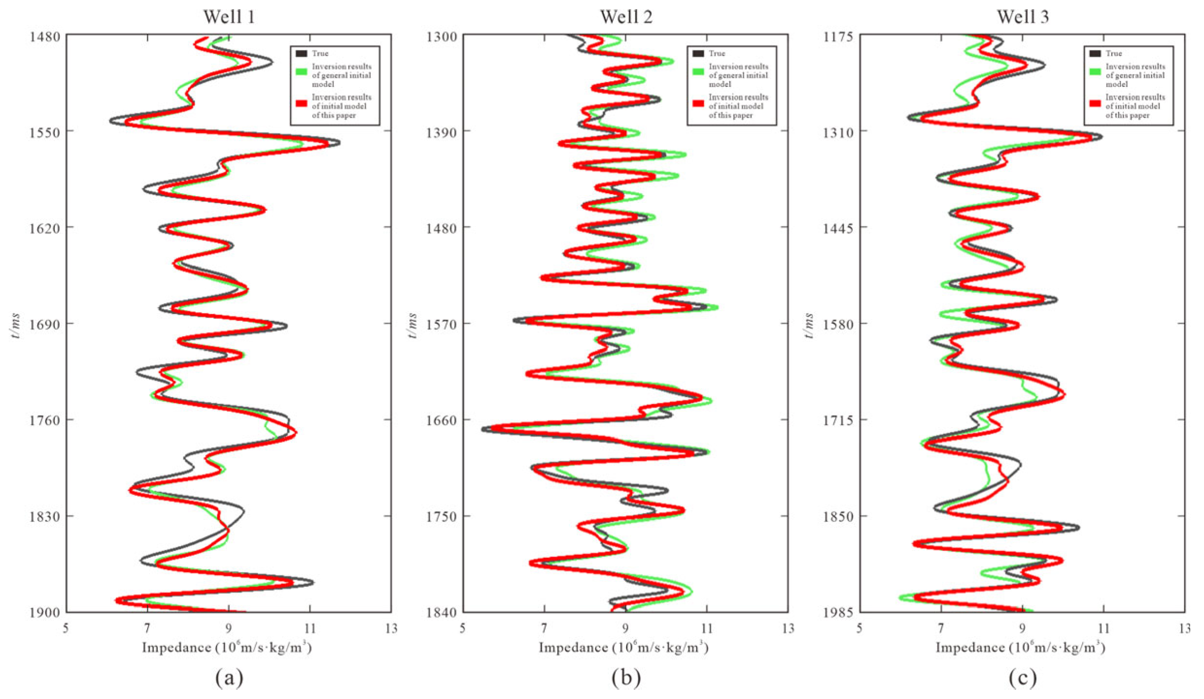
3.2. Comparison of Inversion Results Using Different Initial Low-Frequency Models

Figure 12a shows the high-frequency stratigraphy-constrained facies-controlled LFM proposed in this study. Figure 12b displays the conventional LFM. Figure 12c illustrates the geostatistical inversion results for acoustic impedance using the high-frequency stratigraphy-constrained facies-controlled low-frequency initial model. Figure 12d presents the geostatistical inversion results for acoustic impedance using the conventional low-frequency initial model. Figure 12e shows the geostatistical inversion results for lithology using the high-frequency stratigraphy-constrained facies-controlled low-frequency initial model. Figure 12f illustrates the geostatistical inversion results for lithology using the conventional low-frequency initial model. Although no obvious regional-scale faults or major angular unconformities are visually apparent in the seismic profiles (Figure 12), subtle growth faults and stratigraphic discontinuities are inferred from lateral thickness variations, chaotic reflections, and abrupt seismic facies transitions, especially between Traces 200–400 and 700–850.

The comparison between Figure 12b,c can confirm that the method proposed in this paper can improve the lateral continuity within the same sedimentary phase in LFM while controlling the numerical range of wave impedance locally according to the different sedimentary phases.

Based on the lithology prediction results (Figure 12f), some sand bodies with good continuity and favorable hydrocarbon generation conditions can be predicted (as shown in Figure 12f, Trace = 650 and Trace = 50). In addition, thin-sand predictions can also be well reflected (Trace = 401).

This study uses the tops of Aggradation1, Progradation1, Aggradation2, Progradation2, Retrogradation3, Aggradation3, and Progradation3 from Figure 7 as high-frequency stratigraphy constraints, along with the sedimentary facies defined in Table 1 (including braided-river-delta facies; braided-river-delta-front subfacies; lacustrine- and shallow-lacustrine subfacies; lacustrine, semi-deep, and deep-lacustrine subfacies; and lacustrine–fan facies comprising middle and outer-fan subfacies) to control the initial LFM. The inversion results were then obtained through geostatistical inversion.

As illustrated in Figure 13, the inversion results derived from the conventional low-frequency initial model display reduced vertical resolution, limiting the ability to accurately delineate lithological distributions across various depositional domains. The lateral continuity is poor, and the lateral distribution patterns are unclear, which hinders the ability to represent the distribution of lithology. As a result, the inversion results struggle to capture the characteristics of lithology and sandstone reservoir distribution, as seen in the second section of the Liushagang Formation sandstone reservoir (highlighted by the black box).

In contrast, the inversion results using the high-frequency stratigraphy-constrained facies-controlled low-frequency initial model proposed in this study show a significant improvement in vertical resolution, resulting in a clearer representation of sandstone body distribution and better thin-layer recognition (highlighted by the purple box). The lateral continuity is improved, and the inversion results better align with the sedimentary facies distribution patterns, providing a closer match with actual well-log data. The apparently noisy interval between traces 200–300 (green box) lies beneath a gas-charged shadow zone; however, the inverted acoustic-impedance layer still follows the underlying parallel bedding, validating the robustness of the workflow.

Figure 14 presents the inversion results at three well locations, compared against blind well-log curves along the seismic profile. The comparison indicates that the inver-sion result based on the proposed model (red curve) aligns more closely with the actual well log data (black curve) than the result obtained using the conventional low-frequency initial model (green curve), exhibiting smaller deviations and thereby enhancing the ac-curacy of the seismic inversion.

Figure 15 shows a comparison of lithology inversion results for Well 5. Well 5 is a blind well not involved in the seismic inversion process. The lithology result obtained using the proposed method (Figure 15b) shows high consistency with the true lithology log (Figure 15a). The prediction accuracy rate (89.17%) was calculated based on eight statistical inversions, with a standard deviation of ±2.63%. In contrast, the result from the conventional inversion method (Figure 15c) exhibits noticeable discrepancies from the true lithology, with a lower prediction accuracy of 82.34%. Compared to the conventional approach, the proposed method exhibits improved performance in resolving thin sandstone layers. Nevertheless, accurately differentiating interbedded sandstone and shale sequences remains a challenge. The limit resolution of the lithology prediction results using the method proposed in this paper is approximately 3 m, higher than the limit resolution of 10 m of the traditional methods.

As shown in the results of the computational experiments in Figure 16, the lithology inversion predictions obtained using the method of this paper demonstrate superior performance compared to traditional approaches. Specifically, the prediction accuracies for mudstone, sandstone, and shale all exceed 85% when using the proposed method, whereas the corresponding accuracies for the traditional method remain below 85%. These results indicate that the proposed method achieves a higher overall predictive accuracy, with particularly notable improvements observed in the identification of sandstone.

4. Discussion

In this study, the sequence framework was constructed primarily based on INPEFA inflection points, Morlet wavelet energy changes, and stacking pattern transitions. Although maximum flooding surfaces (MFSs) are traditionally considered key regional correlation markers, they were not explicitly used in this work due to their weak expression and limited lateral continuity in the nearshore lacustrine–deltaic settings of the Wushi Sag. Instead, high-frequency stratigraphy boundaries and stacking patterns were delineated based on more consistent and sensitive log-derived signals to support the inversion-oriented modeling workflow. The retrogradation of SQ2 is not resolved in our dataset; seismic and log evidence suggest that this interval was either non-depositional or subsequently truncated in the proximal near-shore lacustrine setting.

In this study, geostatistical inversion was conducted based on a Bayesian framework combined with a MCMC algorithm. A total of 100 acoustic impedance realizations were generated. For each realization, approximately 60,000 MCMC iterations were performed, including a burn-in phase of 10,000 iterations to ensure convergence of the posterior distribution. The MCMC sampling process adopted a hybrid strategy, utilizing Gibbs sampling to update impedance values across the grid and applying a Metropolis-Hastings criterion to accept or reject proposed updates based on consistency with the observed seismic response. This probabilistic inversion approach enabled the generation of multiple equally probable solutions that integrate well-log constraints, geologic trends, and seismic amplitude data, effectively characterizing the spatial uncertainty of acoustic impedance.

Despite these overall gains, the analysis of Well 6 reveals a key limitation when the target interval lies in a transitional facies zone. The shore–shallow-lake facies encountered by Well 6 shows an impedance range of 6500–8500 m/s·g/cm³ that overlaps extensively with adjacent shallow-lake beach bars (7000–9500 m/s·g/cm³) and deep-lake muds (6000–7500 m/s·g/cm³). This overlap reduces the discriminatory power of truncated Gaussian priors in identifying lithofacies. Therefore, the resolution of seismic inversion results in transitional phase zone strata, and the identification accuracy of lithology prediction, especially for thin layers, still needs to be improved.

Although the proposed workflow is validated in clastic delta–lacustrine systems, it holds potential for adaptation to carbonate reservoirs. In such settings, impedance is primarily controlled by porosity, diagenetic overprinting, and fracture intensity. Therefore, priors must be reconstructed based on porosity clusters rather than only facies zones, and fracture-related anisotropy should be incorporated using multi-point statistics or trend-based variogram models. First, facies-based priors must be reformulated around porosity-controlled impedance distributions. Second, diagenetic overprinting and fracture density should be introduced via multi-point statistics or hierarchical trend models. Third, the likelihood function should be recalibrated to accommodate the higher impedance contrasts of vuggy and tight carbonates. Recent case studies confirm that, with these modifications, geostatistical inversion can be applied successfully to heterogeneous carbonate systems, opening the door to broader deployment of the present workflow beyond the Wushi Sag.

5. Conclusions

This study presents a geostatistical inversion methodology that integrates INPEFA curves and Morlet wavelet transforms, using a high-frequency stratigraphy-constrained facies-controlled low-frequency initial model. The approach was validated using the Marmousi model and applied to sandstone reservoirs in the second and third members of the Liushagang Formation, Wushi Sag. The method improves vertical resolution, lateral continuity, and inversion accuracy compared to conventional models. It also shows strong agreement with actual well-log data, enhancing the prediction reliability of thin sandstone reservoirs in complex depositional settings.

Compared with the studies by Wang, Y. et al. (2024) [19] and Zhu, P. et al. (2023) [20], this work builds upon high-frequency stratigraphy frameworks by incorporating a facies-controlled geostatistical inversion approach. While previous studies relied on Fischer plots and wavelet analysis for sequence boundary identification, this study enhances sequence resolution through the application of Morlet wavelets and INPEFA, enabling more precise stratigraphic division. Furthermore, by integrating seismic and well-log calibrated sedimentary facies models, we achieve a three-dimensional quantitative representation of complex reservoir architectures and extend the applicability of high-frequency stratigraphic framework in spatial modeling.

References

1. Hu, Y.; Xiao, J.; He, W.; Gao, X. Application of high frequency lake level change in the prediction of tight sandstone thin reservoir by sedimentary simulation. Mar. Pet. Geol. 2021, 128, 105049. [Google Scholar] [CrossRef]
2. Fu, C.; Li, S.; Li, S.; Xu, J. Spatial-temporal evolution of the source-to-sink system in the northwestern South China Sea from the Eocene to the Miocene. Glob. Planet. Change 2022, 214, 103851. [Google Scholar] [CrossRef]
3. Gu, Y.; Yin, X.; Zhang, J.; Gu, Y.; Liu, Z. Prediction of reservoir physical parameters based on adaptive step size stochastic inversion. Geoenergy Sci. Eng. 2023, 223, 211455. [Google Scholar] [CrossRef]
4. Hu, W.; Wu, C.; Liang, J.; Hu, F.; Cai, F.; Chai, H.; Zou, Q. Tectonic transport characteristics and their influences on hydrocarbon accumulation in Beibuwan Basin. Oil Gas Geol. 2011, 32, 920–927. [Google Scholar] [CrossRef]
5. Li, C.; Yang, X.; Fan, C.; Hu, L.; Dai, L.; Zhao, S. On the Evolution Process of the Beibu Gulf Basin and Forming Mechanism of Local Structures. Acta Geol. Sin. 2018, 92, 2028–2039. [Google Scholar] [CrossRef]
6. Hao, X.; Ren, Y.; Xu, X.; Liu, H.; Yang, X. Composition Characteristics and Geochemical Significance of Aromatic Hydrocarbon in Crude Oils in Eastern Wushi Sag, Beibu Gulf Basin. Xinjiang Pet. Geol. 2016, 37, 1. [Google Scholar] [CrossRef]
7. Yuan, X.; Yao, G.; Jiang, P.; Lu, J. Provenance Analysis for Liushagang Formation of Wushi Depression, Beibuwan Basin, the South China Sea. Earth Sci. 2017, 42, 2040–2054. [Google Scholar] [CrossRef]
8. Fu, N.; Liu, J. Hydrocarbon generation and accumulation characteristics of three type source rocks of Liu2 segment in Beibuwan Basin. J. Nat. Gas Geosci. 2018, 29, 932–941. [Google Scholar]
9. Sun, L.; Ren, Y.; Qi, Y.; Yu, X.; Li, S.; Zhang, H.; Gao, M.; Yang, K. Analysis of Eocene reservoir characteristics and main controlling factors in Wushi sag, Beibuwan basin. China Offshore Oil Gas 2021, 2, 56–66. [Google Scholar]
10. Wu, K.; Liu, Y.; Hu, D.; Liu, Y.; Zhang, S.; Cui, L. Types and evolution of faults in the east area of the Wushi Sag, Beibuwan Basin. J. Geomech. 2021, 27, 52–62. [Google Scholar] [CrossRef]
11. Wang, Y.; Zhang, H.; Yang, C.; Qi, Z.; Ma, H.; Wang, M.; Chen, J. Sedimentary Model and Its Architectural Characteristics of Delta under the Control of Fault-Rupture-Sag Coupling in Wushi Sag. Spec. Oil Gas Reserv. 2022, 29, 34–41. [Google Scholar]
12. Zeng, X.; Zou, M.; Zhang, H.; Yu, J.; Chen, X.; Mo, F. Main controls on the distribution of the 3rd member of Liushagang Formation in eastern Wushi Sag, Beibu Gulf Basin. Pet. Geol. Exp. 2016, 38, 757–764. [Google Scholar] [CrossRef]
13. Jia, W.; Zong, Z.; Lan, T. Elastic impedance inversion incorporating fusion initial model and kernel Fisher discriminant analysis approach. J. Pet. Sci. Eng. 2023, 220 Pt B, 111235. [Google Scholar] [CrossRef]
14. Jia, W.; Zong, Z.; Qin, D.; Lan, T. Integrated well-log data and seismic inversion results for prediction of hydrocarbon source rock distribution in W segment, Pearl River Mouth Basin, China. Geoenergy Sci. Eng. 2023, 230, 212233. [Google Scholar] [CrossRef]
15. Chen, T.; Zou, B.; Wang, Y.; Cai, H.; Yu, G.; Hu, G. An initial model construction method constrained by stratigraphic sequence representation for pre-stack seismic inversion. Geophys. Prospect. 2024, 72, 2829–2843. [Google Scholar] [CrossRef]
16. Cheng, S.; Zhao, G.; Wang, X.; Wu, Y.; Deng, Z.; Chen, Q.; Xiao, W.; Huang, H.; Tang, Y. Thin reservoir seismic prediction method based on high resolution sequence constraint. Prog. Geophys. 2024, 39, 606–619. [Google Scholar] [CrossRef]
17. Neal, J.E.; Abreu, V.; Bohacs, K.M.; Feldman, H.R.; Pederson, K.H. Accommodation succession (δA/δS) sequence stratigraphy: Observational method, utility and insights into sequence boundary formation. J. Geol. Soc. Lond. 2016, 173, 803–816. [Google Scholar] [CrossRef]
18. Xu, C.; Gong, C.; Ronald, J.S.; Zhang, X.; Guan, D.; Li, D. Predicting the occurrence and development of regionally extensive sublacustrine fans in the Oligocene Bohai Bay Basin: From sequence stratigraphy to source-to-sink systems. AAPG Bull. 2025, 109, 307–334. [Google Scholar] [CrossRef]
19. Wang, Y.; Ge, X.; Tang, P.; Yang, B.; Chen, D.; Deng, M.; Zhao, G. Division of the Sequence Stratigraphy of the Sinian Qigebrak Formation in the Northwest Tarim Basin-Evidence from the High-resolution Analysis of Depositional Facies and the Fischer Plot. Acta Sedimentol. Sin. 2024, 40, 1. [Google Scholar] [CrossRef]
20. Zhu, P.; Ma, T.; Wang, X.; Li, X.; Dong, Y.; Yang, W.; Teng, Z. Wavelet transform coupled with Fischer plots for sequence stratigraphy: A case study in the Linxing area, Ordos Basin, China. Geoenergy Sci. Eng. 2023, 231 Pt A, 212306. [Google Scholar] [CrossRef]
21. Hu, Y.; He, W.; Guo, B. Combining sedimentary forward modeling with sequential Gauss simulation for fine prediction of tight sandstone reservoir. Mar. Pet. Geol. 2020, 112, 104044. [Google Scholar] [CrossRef]
22. Yuan, R.; Zhu, R.; Qu, J.; Wu, J.; You, X.; Sun, Y.; Zhou, Y. Utilizing Integrated Prediction Error Filter Analysis (INPEFA) to divide base-level cycle of fan-deltas: A case study of the Triassic Baikouquan Formation in Mabei Slope Area, Mahu Depression, Junggar Basin, China. Open Geosci. 2018, 10, 79–86. [Google Scholar] [CrossRef]
23. Yuan, Y.; Wang, L.; Xie, R. Application of INPEFA technology to sequence stratigraphy of the third member of Funing Formation, Nanhua block, Qintong Sag, North Jiangsu Basin. Pet. Geol. Exp. 2018, 40, 871–876. [Google Scholar] [CrossRef]
24. Zhou, Y.; Du, Y.; Xie, J.; Guo, F.; Zhang, S. Application and comparison of INPEFA technique and wavelet transform in sequence stratigraphic division: A case study in the third member of Dongying formation in Dawangzhuang area, Raoyang sag. China Sci. 2021, 05, 494–501. [Google Scholar] [CrossRef]
25. Zhu, H.; Huang, Z.; Liu, H.; Liu, K.; Liu, Q. Progress and developing tendency of technologies and methods used to recognise sequence stratigraphic units based on the well-log data. Geol. Sci. Technol. Inf. 2011, 30, 29–36. [Google Scholar] [CrossRef]
26. Fu, Z.; Yin, C.; Chen, T.; Ji, Y.; Liao, J. Using the wavelet transform for seismic wave impedance inversion. Geophysics 2024, 89, R387–R397. [Google Scholar] [CrossRef]
27. Lin, Z.; Liao, J.; Liu, X.; Wang, P.; Gao, Y.; Li, J. A high resolution inversion method for fluid factor with dynamic dry-rock VP/VS ratio squared. Pet. Sci. 2023, 20, 2822–2834. [Google Scholar] [CrossRef]
28. Dong, H.; Liu, J.; Li, Y.; Shi, C. The division of Triassic sequence and analysis of lacustrine level changes in Tarim Basin Based on Wavelet Transform. Sci. Technol. Eng. 2023, 23, 54–65. [Google Scholar] [CrossRef]
29. Bi, Z.; Wu, X.; Li, Y.; Yan, S.; Zhang, S.; Si, H. Geologic-time-based interpolation of borehole data for building high-resolution models: Methods and applications. Geophysics 2022, 87, IM67–IM80. [Google Scholar] [CrossRef]
30. Dong, S.; Zeng, L.; Du, X.; He, J.; Sun, F. Lithofacies identification in carbonate reservoirs by multiple kernel Fisher discriminant analysis using conventional well logs: A case study in A oilfield, Zagros Basin, Iraq. J. Pet. Sci. Eng. 2022, 210, 110081. [Google Scholar] [CrossRef]
31. Dong, S.; Wang, Z.; Zeng, L. Lithology identification using kernel Fisher discriminant analysis with well logs. J. Pet. Sci. Eng. 2016, 143, 95–102. [Google Scholar] [CrossRef]
32. Liu, X.; Li, J.; Chen, X.; Zhou, L.; Guo, K. Bayesian discriminant analysis of lithofacies integrate the Fisher transformation and the kernel function estimation. Interpret.-J. SUB 2017, 5, SE1–SE10. [Google Scholar] [CrossRef]
33. Sarah, K.S.; James, A.M.; Octavian, C.; Shahin, E.D.; Nakarí, D. High-resolution sequence stratigraphic framework for the late Albian Viking Formation in central Alberta. Mar. Pet. Geol. 2022, 139, 105627. [Google Scholar] [CrossRef]
34. Yan, J.; Cai, J.; Zhao, M.; Zheng, D. Advances in the study of sequence stratigraphic division and correlation using well log information. J. Stratigr. 2009, 33, 441–450. [Google Scholar] [CrossRef]
35. Hesam, K.A. Estimation of Petroleum Reservoir Parameters Using an Integrated Approach Neural Network, Principal Component Analysis and Fisher Discriminant Analysis. Pet. Sci. Technol. 2013, 315, 530–539. [Google Scholar] [CrossRef]
36. Yuan, H.; Qu, X.; Bao, K. Complex frequency domain seismic inversion method for well-free area based on geological model. Oil Geophys. Prospect. 2024, 59, 558–566. [Google Scholar] [CrossRef]
37. Sun, Q.; Zong, Z. Building initial model for seismic inversion based on semi-supervised learning. Geophys. Prospect. 2024, 72, 1800–1815. [Google Scholar] [CrossRef]
38. Srivastava, R.; Sen, M. Stochastic inversion of prestack seismic data using fractal-based initial models. Geophysics 2010, 75, R47–R59. [Google Scholar] [CrossRef]
39. Wu, W.; Li, Q.; Pei, J.; Ning, S.; Tong, L.; Liu, W.; Feng, Z. Seismic sedimentology, facies analyses, and high-quality reservoir predictions in fan deltas: A case study of the Triassic Baikouquan Formation on the western slope of the Mahu Sag in Chinese Junggar Basin. Mar. Pet. Geol. 2020, 120, 104546. [Google Scholar] [CrossRef]
40. Xu, X.; Hu, L.; Man, Y.; Xue, H.; Li, A. Sand control model and exploration practice for East Wushi Sag strike slope. J. Southwest Pet. Univ., Sci. Technol. Ed. 2017, 39, 77–84. [Google Scholar]
41. Li, J.; Chen, Z.; Wang, L.; Liu, L.; Li, J. Application of facies-controlled technique to bioclastic shoal reservoir prediction in less well zones. Lithol. Reserv. 2017, 29, 110–117. [Google Scholar] [CrossRef]
42. Leisi, A.; Shad, M.N. Three-dimensional shear wave velocity prediction by integrating post-stack seismic attributes and well logs: Application on Asmari formation in Iran. J. Pet. Explor. Prod. Technol. 2024, 14, 2399–2411. [Google Scholar] [CrossRef]
43. Zhang, Y.; Zhou, H.; Zhang, M.; Wang, Y.; Feng, B.; Liang, M. Structurally Constrained Initial Impedance Modeling for Poststack Seismic Inversion. IEEE Trans. Geosci. Remote Sens. 2023, 61, 5906310. [Google Scholar] [CrossRef]
44. Li, H.; Li, W.; Liu, J.; Gong, W.; Zhang, W. Two-step facies-constrained inversion in prediction of carbonate rock fault-controlled reservoirs with post stack seismic in No.8 structure of Shunbei block, Tarim Basin. Nat. Gas Geosci. 2023, 11, 1961–1970. [Google Scholar] [CrossRef]
45. Liu, Z.; Song, W.; Chen, X.; Li, W.; Li, Z.; Liu, G. High-resolution reservoir prediction method based on data-driven and model-based approaches. Geophys. Prospect. 2024, 72, 1971–1984. [Google Scholar] [CrossRef]
46. Michael, R.; Bahk, J.J.; Kim, H.S.; Scholz, N.A.; Yoo, D.G.; Kim, W.S.; Ryu, B.J.; Lee, S.R. Seismic facies analyses as aid in regional gas hydrate assessments, Part-II: Prediction of reservoir properties, gas hydrate petroleum system analysis, and Monte Carlo simulation. Mar. Pet. Geol. 2013, 47, 269–290. [Google Scholar] [CrossRef]
47. Catuneanu, O. Principles of Sequence Stratigraphy, 2nd ed.; Elsevier: Amsterdam, The Netherlands, 2022; p. 496. [Google Scholar]
48. Chen, T.; Liang, J.; Li, P.; Cai, H.; Hu, G.; Wang, Y. Geostatistical seismic inversion constrained by reservoir sedimentary structural features. Geophysics 2022, 87, 1942–2156. [Google Scholar] [CrossRef]
49. Xue, H.; Li, J.; Li, S.; Wang, M.; Sun, Z.; Yu, T. Application of INPEFA Technique to Research High Resolution Sequence Stratigraphy:as an Example of Youfangzhuang Area Chang 4+5in Ordos Basin. Period. Ocean Univ. China 2015, 45, 101–106. [Google Scholar] [CrossRef]
50. Li, W.; Zhang, J.; Xie, J.; Xia, Y.; He, Y. Application of the Wavelet Transform and INPEFA in Sequence Stratigraphy. ACS Omega 2023, 8, 3441–3451. [Google Scholar] [CrossRef]
51. Chen, X.; Tian, X.; Shi, J.; Wang, X.; Xiong, Y.; Wang, K.; Wang, N.; Zhang, H.; Zhao, H.; Qian, H. Sequence Stratigraphic Division Based on Wavelet Transform and Its Control on Favorable Reservoirs in the Hechuan-Tongnan Area of the Sichuan Basin: A Case Study of the Fourth Member of the Dengying Formation in the Sinian System. Pet. Geol. Oilfield Dev. Daqing 2025, 44, 41–49. [Google Scholar] [CrossRef]
52. Hu, D.; Deng, Y.; Zhang, J.; Zuo, Q.; He, W. Palaeogene fault system and hydrocarbon accumulation in East Wushi Sag. J. Southwest Pet. Univ. Sci. Technol. Ed. 2016, 38, 27–36. [Google Scholar]
53. Chen, J.; Chen, X.; Liu, X.; Chen, S.; Li, C. Lithofacies Discrimination Based On Adaptive Kernel Function of Support Vector Machines. In Proceedings of the 80th EAGE Conference and Exhibition 2018, Copenhagen, Denmark, 11–14 June 2018; pp. 1–5. [Google Scholar] [CrossRef]
54. Liu, X.; Chen, X.; Li, J.; Zhou, L.; Li, C. Reservoir Properties Prediction Based on Support Vector Regression with Optimized Parameters by Quantum Particle Swarm. In Proceedings of the 81st EAGE Conference and Exhibition 2019, London, UK, 3–6 June 2019; Volume 1, pp. 1–5. [Google Scholar] [CrossRef]
55. Liu, X.; Shao, G.; Yuan, C.; Chen, X.; Li, J.; Chen, Y. Mixture of relevance vector regression experts for reservoir properties prediction. J. Pet. Sci. Eng. 2022, 214, 110498. [Google Scholar] [CrossRef]
56. Lyu, P.; Liu, C.; Yan, K.; Zhang, J. Study on the seismic facies of the Shahezi formation in Xujiaweizi fault depression in Songliao basin. Geol. Resour. 2014, 23, 330–334. [Google Scholar] [CrossRef]
57. Liu, X.; Chen, X.; Li, J.; Zhou, X.; Chen, Y. Facies Identification Based on Multikernel Relevance Vector Machine. IEEE Trans. Geosci. Remote Sens. 2020, 58, 7269–7282. [Google Scholar] [CrossRef]
58. Liu, X.; Li, B.; Li, J.; Chen, X.; Li, Q.; Chen, Y. Semi-supervised deep autoencoder for seismic facies classification. Geophys. Prospect. 2021, 69, 1295–1315. [Google Scholar] [CrossRef]
59. Liu, X.; Zhou, L.; Chen, X.; Li, J. Lithofacies identification using support vector machine based on local deep multi-kernel learning. Pet. Sci 2020, 17, 954–966. [Google Scholar] [CrossRef]
60. Nurul, A.M.; Meor, H.A. Seismic geomorphological analysis of channel types: A case study from the Miocene Malay Basin. J. Geophys. Eng. 2023, 20, 159–171. [Google Scholar] [CrossRef]
61. Feng, R.; Stefan, M.L.; Dries, G.; Erika, A. Reservoir lithology classification based on seismic inversion results by Hidden Markov Models: Applying prior geological information. Mar. Pet. Geol. 2018, 93, 218–229. [Google Scholar] [CrossRef]
62. Maurya, S.P.; Richa; Singh, K.H.; Mahadasu, P.; Ajay, P.S.; Hema, G.; Kushwaha, P.K.; Raghav, S. Prediction of acoustic impedance and density porosity using seismic inversion, and geostatistical methods on Krishna Godavari basin, India: A case study. J. Appl. Geophys. 2023, 219, 105237. [Google Scholar] [CrossRef]
63. Fang, G.; Enhedelihai, A.N.; Li, Y.E.; Tan, Y.; Cheng, A. Quantifying tunneling risks ahead of TBM using Bayesian inference on continuous seismic data. Tunn. Undergr. Space Technol. 2024, 147, 105702. [Google Scholar] [CrossRef]
64. Chen, L.; Liu, X.; Zhou, H.; Zhang, H.; Lyu, F.; Mo, Q. Identification of Carbonate Cave Reservoirs Based on Variational Bayesian Principal Component Analysis. IEEE Trans. Geosci. Remote Sens. 2023, 61, 5922910. [Google Scholar] [CrossRef]
65. Liu, X.; Chen, X.; Li, J.; Zhou, L.; Guo, K. Reservoir physical property prediction based on kernel-Bayes discriminant method. Acta Pet. Sin. 2016, 37, 878–886. [Google Scholar]
66. Yang, Z.; Gao, Z.; Liu, X. Seismic impedance inversion of coal field with reflectivity method based on Bayesian theory. Coal Geol. Explor. 2020, 48, 204–210. [Google Scholar] [CrossRef]
67. Wang, Z.; Wang, S.; Li, Z.; Zhou, C.; Wang, Z. AVO Uncertainty Inversion Based on Multitask Variational Bayesian Neural Network. IEEE Trans. Geosci. Remote Sens. 2024, 62, 5925816. [Google Scholar] [CrossRef]
68. Amira, Z.; Adnen, A.; Nesserine, B.; Mohamed, A.B.; Mohamed, H.I. Integrated seismic inversion for clastic reservoir characterization: Case of the upper Silurian reservoir, Tunisian Ghadames Basin. J. Appl. Geophys. 2023, 219, 105252. [Google Scholar] [CrossRef]
69. Garia, S.; Pal, A.K.; Katre, S.; Nayak, S.; Ravi, K.; Nair, A.M. Seismic coloured inversion to explore the hydrocarbon prospectivity of a field in the Upper Assam basin. Explor. Geophys. 2024, 55, 752–774. [Google Scholar] [CrossRef]
70. Lin, Y.; Wang, B.; Huang, M.; Chen, S.; Zhao, C. An improved stochastic inversion method for 3D elastic impedance under the prior constraints of random medium parameters. Geoenergy Sci. Eng. 2024, 233, 212421. [Google Scholar] [CrossRef]
71. Ge, Q.; Cao, H.; Yang, Z.; Li, X.; Yan, X.; Zhang, X.; Wang, Y.; Lu, W. High-resolution seismic impedance inversion integrating the closed-loop convolutional neural network and geostatistics: An application to the thin interbedded reservoir. J. Geophys. Eng. 2022, 19, 550–561. [Google Scholar] [CrossRef]
72. Liu, X.; Li, J.; Chen, X.; Li, C.; Guo, K.; Zhou, L. A stochastic inversion method integrating multi-point geostatistics and sequential Gaussian simulation. Chin. J. Geophys. 2018, 61, 2998–3007. [Google Scholar] [CrossRef]
73. Liu, X.; Li, J.; Chen, X.; Guo, K.; Li, C.; Zhou, L.; Cheng, J. Stochastic inversion of facies and reservoir properties based on multi-point geostatistics. J. Geophys. Eng. 2018, 15, 2455–2468. [Google Scholar] [CrossRef]
74. Zhou, L.; Liu, X.; Li, J.; Liao, J. Robust AVO inversion for the fluid factor and shear modulus. Geophysics 2021, 86, R471–R483. [Google Scholar] [CrossRef]
75. Singh, R.; Srivastava, A.; Kant, R. Integrated thin layer classification and reservoir characterization using sparse layer reflectivity inversion and radial basis function neural network: A case study. Mar. Geophys. Res. 2024, 45, 3. [Google Scholar] [CrossRef]
Figure 1. Location of Wushi Sag in Beibu Gulf Basin, China.
Jmse 13 01390 g001
Figure 2. Flowchart for initial low-frequency model construction.
Jmse 13 01390 g002
Figure 3. The INPEFA curve calculation process of Well 5. (a) GR; (b) MESA; (c) PEFA; (d) INPEFA. Note: Blue arrows stand for the negative excursions of the INPEFA curve. Red arrows stand for the positive excursions of the INPEFA curve. Wedges Abrupt shifts stand for erosive or flooding surfaces associated with SB and TS.
Jmse 13 01390 g003
Figure 4. Comparison between the GR curve and Morlet wavelet transforms of Well 6 with different scale sizes. (a) GR curve; (b) Morlet (scale = 256); (c) Morlet (scale = 128); (d) Morlet (scale = 64). Note: Yellow arrows stand for the transitions in the Morlet wavelet energy blobs from low to high values. Red arrows stand for the transitions in the Morlet wavelet energy blobs from high to low values.
Jmse 13 01390 g004
Figure 5. Results of multi-parameter stratigraphic framework division for Well 3, Well 13, and Well 14.
Jmse 13 01390 g005
Figure 6. Stratigraphic framework establishment process through Well 14. (a) Sequence stratigraphic division results; (b) time–depth conversion and well-seismic calibration; (c) sequence stratigraphic framework establishment results. Note: Blue dash lines stand for the top of retrogradation. Green dash lines stand for the top of aggradation. Black lines stand for the top of progradation.
Jmse 13 01390 g006
Figure 7. (a) Well-to-well lithofacies stratigraphic framework division and (b) stratigraphic framework construction. Note: Blue dash lines stand for the top of retrogradation. Green dash lines stand for the top of aggradation. Black lines stand for the top of progradation. Red lines stand for the faults.
Jmse 13 01390 g007
Figure 8. Model test effect comparison chart. (a) Ture model; (b) synthetic seismic recordings; (c) general initial model; (d) initial model of methodology in this paper; (e) inversion results of general initial model; (f) inversion results of initial model of methodology in this paper.
Jmse 13 01390 g008
Figure 9. Comparison of inversion results. (a) Trace = 1290; (b) Trace = 2004; (c) Trace = 2115.
Jmse 13 01390 g009
Figure 10. Present-day lithofacies distribution and interpreted depositional environments of Retrogradation3. Note: The map depicts the present-day distribution of lithofacies. No palinspastic restoration has been applied; therefore, fault-related displacement has not been back-stripped.
Jmse 13 01390 g010
Figure 11. Comparison of the well-connected sedimentary facies section with the initial low-frequency model. (a) Well-connected sedimentary facies section; (b) initial low-frequency model section. Note: Black lines stand for the well-log of wells.
Jmse 13 01390 g011
Figure 12. Comparison of initial low-frequency models and inversion results. (a) Seismic; (b) low-frequency model of this paper; (c) traditional low-frequency model; (d) impedance inversion results of this paper; (e) traditional impedance inversion results; (f) lithology prediction inversion results of this paper; (g) traditional lithology prediction inversion results. Note: Black lines stand for the faults.
Jmse 13 01390 g012
Figure 13. Comparison of inversion outputs from different LFMs. (a) Seismic with well path; (b) traditional impedance inversion results; (c) traditional lithology prediction inversion results; (d) impedance inversion results of this paper; (e) lithology prediction inversion results of this paper.
Jmse 13 01390 g013
Figure 14. Comparison of wave impedance curves of inversion results. (a) Curve comparison chart of Well 1; (b) curve comparison chart of Well 2; (c) curve comparison chart of Well 3.
Jmse 13 01390 g014
Figure 15. Comparison between the inverted lithology results and the blind well log of Well 7. (a) True lithology log of Well 7; (b) lithology prediction inversion results of this paper; (c) traditional lithology prediction inversion results.
Jmse 13 01390 g015
Figure 16. A comparison chart of the confusion matrices of the two inversion lithology results of blind wells. (a) Lithology prediction inversion results of this paper; (b) traditional lithology prediction inversion results.
Jmse 13 01390 g016