Improved Super-Twisting Sliding Mode Control of a Brushless Doubly Fed Induction Generator for Standalone Ship Shaft Power Generation Systems

Abstract

This study proposes an improved super-twisting sliding mode (STSM) control method for a brushless doubly fed induction generator (BDFIG) used in standalone ship shaft power generation systems. Focusing on the problem of the low tracking accuracy of the power winding (PW) voltages caused by the parameter perturbation of BDFIG systems, a mismatched uncertain model of the BDFIG is constructed. Additionally, an improved STSM control method is proposed to address the power load variation and compensate for the mismatched uncertainty through virtual control technology. Based on the direct vector control of the control winding (CW), the proposed method ensured that the voltage amplitude error of the power winding could converge to the equilibrium point rather than the neighborhood. Finally, in the experimental investigation of the BDFIG-based ship shaft independent power system, the dynamic performance in the startup and power load changing conditions were analyzed. The experimental results show that the proposed improved STSM controller has a faster dynamic response and higher steady-state accuracy than the proportional integral control and the linear sliding mode control, with strong robustness to the mismatched uncertainties caused by parameter perturbations.

1. Introduction

Increasing the efficiency of energy utilization has been emphasized with the diminishing availability of traditional fossil energy reserves. Within the maritime industry, there has been a growing adoption of shaft power generation technology to optimize energy efficiency while minimizing operational costs. The brushless doubly fed induction generator (BDFIG) has been found to increase utilization in constant-voltage constant-frequency variable-speed generation systems, particularly due to its brushless design, which eliminates the need for slip rings [1,2]. This feature significantly enhances the reliability and safety of the system, making it a promising solution for energy conversion in maritime applications. Consequently, integrating BDFIGs into ship propulsion systems has caused widespread concern [3,4].

The complex structure and the severe coupling of BDFIG lead to its control difficulties [5]. Due to the variability of the marine environment and climate, the temperature and frequency of BDFIG change [6]. The motor parameters are disturbed, affecting the control accuracy. At the same time, in some cold areas, the ship breaking the ice barrier will also make the motor suffer from load disturbance [7]. Therefore, the control strategy of the BDFIG requires strong robustness.

Much attention is paid to novel control strategies for the application of BDFIG. The vector control (VC) system possesses better dynamic performance by controlling the active and reactive powers of BDFIG [8,9,10]. However, the VC-based controller requires the appropriate decoupling of the system and is therefore sensitive to the presence of the inner parameters perturbations. The direct torque control [11] and direct power control [12,13] methods enhance the robustness of the control system. In contrast, the control is not optimal in real-time when selecting a predefined voltage vector. Moreover, this method may cause torque/power ripples and current waveform distortion.

The controller oriented with the CW-side current is proposed to reduce the influence of voltage fluctuation on the PW-side and has stronger robustness than traditional PW-oriented controllers [5]. Furthermore, by taking the Taylor expansion at the equilibrium point of PW-side voltage, the outer loop is transformed into a linear subsystem, and the control complexity is simplified. However, the uncertainties from model simplification and the mismatched parameter perturbations still exist, which could affect the dynamic response and precision of the controls.

Traditional control methods, such as PI or PID control, achieve the asymptotical convergence of the system by adjusting the proportional, integral and differential gains; they struggle to ensure the high accuracy of the uncertain systems with complex disturbances [14]. Adaptive disturbance rejection control (ADRC) and the disturbance-observer-based (DOB) control methods are proposed to compensate disturbances by using observers, while these methods are sensitive to parameter perturbations [15]. Due to the significant advantages of robustness and parameter insensitivity, SMC methods are used widely for uncertain nonlinear systems [16].

Integral sliding mode control (ISMC) can enhance the control accuracy, and terminal sliding mode control (TSMC) is capable of guaranteeing finite-time convergence while maintaining high precision [17,18]. Meanwhile, these traditional SMC methods suffer from the chattering problem. The chattering leads to the high-frequency switching of control signals because of the sign term in the traditional SMC law [19]. To eliminate the chattering, standard super-twisting sliding mode control (STSM) was designed [20,21,22]. The STSM control methods are widely used in practical applications, with strong robustness against perturbations and chattering-free characteristic [23]. However, the standard STSMs fail to compensate for the mismatched uncertainties, which limits their application in industrial control systems, such as BDFIG control systems.

This article proposes an improved STSM control algorithm combined with the virtual control law to compensate for the mismatched uncertainties caused by parameter perturbations, which guarantee the robustness and quick dynamic response of the controller. The innovation of the study can be outlined as follows:

(1)

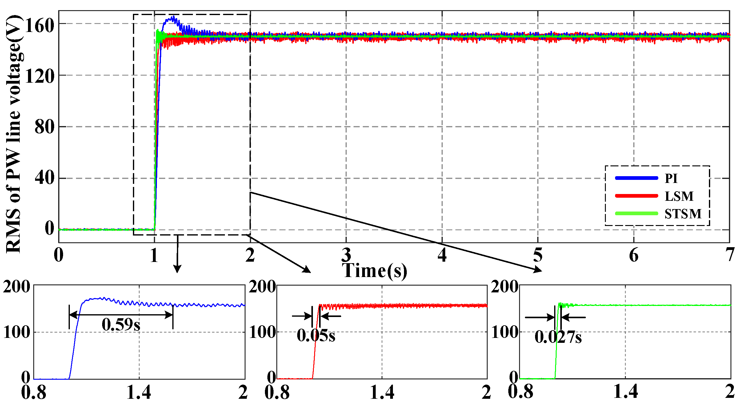
Compared with traditional controllers, the improved STSM control method avoids the low-pass filter and improves the transient response of the terminal voltage.

(2)

The matched and mismatched uncertainties in BDFIG-based ship shaft power generation systems are considered and compensated.

The study is organized as follows. Section 2 describes the BDFIG mathematical model with parameter perturbation uncertainties. The main contribution of this research is presented in Section 3, which comprises the design of the super-twisting sliding mode controller (STSMC) and the stability analysis based on Lyapunov theory. Section 4 shows the experimental results and the rapidness and robustness of the uncertainties of the BDFIG control system. Finally, Section 5 presents the conclusions.

2. BDFIG Mathematical Model with Perturbations

2.1. Traditional BDFIG Model

While BDFIG operates for an independent power generation system, the PW is connected to a load rather than a power grid. The traditional PW-side voltage orientation control method ignores the fluctuation of PW-side voltage. In this article, the rotation frequency of the d–q coordinates is set as the angle frequency of CW to enhance the effectiveness of the control system.

The stator voltage function of the PW is given as follows:

$$\left\{\begin{array}{l}{u}_{sd}=R_{sd}{i}_{sd}+{\displaystyle \frac{d{\psi }_{sd}}{dt}}-{\omega }_{s1}{\psi }_{sq}\\ u_{sq}=R_{sq}{i}_{sq}+{\displaystyle \frac{d{\psi }_{sq}}{dt}}+{\omega }_{s1}{\psi }_{sd}\end{array}\right.$$

(1)

where u_sd and u_sq, respectively, represent the stator voltage of PW in the d- and q-axes, i_sd and i_sq are the stator current of the PW, R_sd and R_sq are the stator resistance of the PW, ψ_sd and ψ_sq the stator flux of the PW, and ω_s1 is the angular frequency of the CW.

The stator flux function of the PW is presented as:

$$\left\{\begin{array}{l}{\psi }_{sd}=L_{sd}{i}_{sd}+L_{sr}{i}_{rd}\\ {\psi }_{sq}=L_{sq}{i}_{sd}+L_{sr}{i}_{rq}\end{array}\right.$$

(2)

where i_rd and i_rq, respectively, represent the rotor current in the d- and q-axes, L_s is the self-inductance of PW, and L_sr the mutual inductance between the PW and the rotor.

The stator voltage function of the CW is:

$$\left\{\begin{array}{l}{u}_{s1d}=R_{s1d}{i}_{s1d}+{\displaystyle \frac{d{\psi }_{s1d}}{dt}}-\left[{\omega }_{s1}-\left(p_s+p_{s1}\right){\omega }_r\right]{\psi }_{s1q}\\ u_{s1q}=R_{s1q}{i}_{s1q}+{\displaystyle \frac{d{\psi }_{s1q}}{dt}}+\left[{\omega }_{s1}-\left(p_s+p_{s1}\right){\omega }_r\right]{\psi }_{s1d}\end{array}\right.$$

(3)

where u_s1d and u_s1q, respectively, represent the stator voltage of CW in the d- and q-axes, i_s1d and i_s1q are the stator current of CW, R_s1d and R_s1q correspond to the stator resistance of CW, ψ_s1d and ψ_s1q represent the stator flux of CW, p_s and p_s1, respectively, represent the number of pole pairs in PW side and the CW side, and ω_r is the angular frequency of the rotor.

The stator flux of CW can be presented as:

$$\left\{\begin{array}{l}{\psi }_{s1d}=L_{s1}{i}_{s1d}+L_{s1r}{i}_{rd}\\ {\psi }_{s1q}=L_{s1}{i}_{s1d}+L_{s1r}{i}_{rq}\end{array}\right.$$

(4)

where L_s1 represents the self-inductances of CW, and L_s1r represents the mutual inductance between the CW and the rotor.

The voltage function of the rotor can be expressed as:

$$\left\{\begin{array}{l}{u}_{rd}=R_{rd}{i}_{rd}+{\displaystyle \frac{d{\psi }_{rd}}{dt}}+\left({\omega }_s-p_{s1}{\omega }_r\right){\psi }_{rq}\\ u_{rq}=R_{rq}{i}_{rq}+{\displaystyle \frac{d{\psi }_{rq}}{dt}}-\left({\omega }_s-p_{s1}{\omega }_r\right){\psi }_{rd}\end{array}\right.$$

(5)

where u_rd and u_rq, respectively, represent the rotor voltage in the d- and q-axes, R_rd and R_rq correspond to the rotor resistance, ψ_rd and ψ_rq are the rotor flux, and ω_s is the angular frequency of PW.

The rotor flux function is:

$$\left\{\begin{array}{l}{\psi }_{rd}=L_r{i}_{rd}+L_{sr}{i}_{sd}+L_{s1r}{i}_{s1d}\\ {\psi }_{rq}=L_r{i}_{rd}+L_{sr}{i}_{sd}+L_{s1r}{i}_{s1q}\end{array}\right.$$

(6)

where L_r represents the self-inductances of the rotor.

Under a stable doubly fed operation mode, the shaft speed is satisfied as follows:

$${\omega }_r={\displaystyle \frac{{\omega }_s+{\omega }_{s1}}{p_s+p_{s1}}}$$

(7)

The rotor voltage is satisfied with u_rd = u_rq = 0 when the load is a three-phase symmetric load. Combined with (5) and (6), the rotor current can be expressed as:

$$\begin{array}{ll}{i}_{rd}& =-{\displaystyle \frac{\left[s^2+\left(R_r/L_r\right)s+{\left({\omega }_s-p_{s1}{\omega }_r\right)}^2\right]\left(L_{sr}{i}_{sd}+L_{s1r}{i}_{s1d}\right)}{L_r\left[s^2+2\left(R_r/L_r\right)s+{\left({\omega }_s-p_{s1}{\omega }_r\right)}^2\right]}}\\ & -{\displaystyle \frac{R_r\left({\omega }_s-p_{s1}{\omega }_r\right)\left(L_{sr}{i}_{sq}+L_{s1r}{i}_{s1q}\right)}{{\left(R_r+L_{r}s\right)}^2+L_r^2{\left({\omega }_s-p_{s1}{\omega }_r\right)}^2}}\end{array}$$

(8)

$$\begin{array}{ll}{i}_{rq}& ={\displaystyle \frac{\left({\omega }_s-p_{s1}{\omega }_r\right)}{R_r+L_{r}s}}\left[1-{\displaystyle \frac{L_r^2{s}^2+L_r{R}_{r}s+L_r^2{\left({\omega }_s-p_{s1}{\omega }_r\right)}^2}{{\left(R_r+L_{r}s\right)}^2+L_r^2{\left({\omega }_s-p_{s1}{\omega }_r\right)}^2}}\right]\left(L_{sr}{i}_{sd}+L_{s1r}{i}_{s1d}\right)\\ \hspace{1em}& -{\displaystyle \frac{\left(L_{sr}{i}_{sq}+L_{s1r}{i}_{s1q}\right)}{R_r+L_{r}s}}\left[s+{\displaystyle \frac{L_r{R}_r{\left({\omega }_s-p_{s1}{\omega }_r\right)}^2}{{\left(R_r+L_{r}s\right)}^2+L_r^2{\left({\omega }_s-p_{s1}{\omega }_r\right)}^2}}\right]\end{array}$$

(9)

where s represents the differential operator. Compared to the self-induction of rotor winding, the rotor resistance is small enough to be neglected. Thus, the pole is approximately equal to zero for the first part in (8), which can be simplified as −(L_sri_sd + L_s1ri_s1d)/L_r. In the rest, the term (R_r + L_rs)² is small enough to be neglected as well. Finally, the rotor d-axis current (8) is simplified as:

$$i_{rd}=-{\displaystyle \frac{L_{sr}{i}_{sd}+L_{s1r}{i}_{s1d}}{L_r}}-{\displaystyle \frac{R_r\left(L_{sr}{i}_{sq}+L_{s1r}{i}_{s1q}\right)}{L_r^2{\left({\omega }_s-p_{s1}{\omega }_r\right)}^2}}$$

(10)

Similarly, the rotor q-axis current (9) can be simplified as:

$$i_{rq}={\displaystyle \frac{L_{sr}{i}_{sq}+L_{s1r}{i}_{s1q}}{L_r}}$$

(11)

Substituting Equations (4), (7), (10) and (11) into Equation (3), the voltage of CW can be obtained as:

$$\left\{\begin{array}{l}{u}_{s1d}={\sigma }_{s1}{L}_{s1}{\displaystyle \frac{d{i}_{s1d}}{dt}}+R_{s1}{i}_{s1d}+D_{s1d}\\ u_{s1q}={\sigma }_{s1}{L}_{s1}{\displaystyle \frac{d{i}_{s1q}}{dt}}+R_{s1}{i}_{s1q}+D_{s1q}\end{array}\right.$$

(12)

where σ_s1 = 1 − L²_s1r/(L_s1 L_r) is defined by the leakage inductance of CW, and D_s1d = α₁i_s1q + α₂i_sd + α₃i_1q and D_s1q = α₄i_s1d + α₅i_sd + α₆i_sq represent the cross disturbance of the d and q components, where:

$$\begin{array}{l}{\alpha }_1={\displaystyle \frac{{\omega }_s\left({\omega }_s-p_{s1}{w}_r\right)\left(L_r^2{L}_{s1}+L_{s1r}^2{L}_r\right)-L_{s1r}^2{R}_{r}s}{L_r^2\left({\omega }_s-p_{s1}{w}_r\right)}}\hspace{1em}\hspace{1em}\hspace{1em}\hspace{1em}, \hspace{1em}\hspace{1em}\hspace{1em}\hspace{1em}\hspace{1em}\hspace{1em}{\alpha }_2=-{\displaystyle \frac{L_{sr}{L}_{s1r}s}{L_r}} \hspace{1em}\hspace{1em}\hspace{1em}\hspace{1em}\hspace{1em}\hspace{1em},\\ {\alpha }_3={\displaystyle \frac{L_{sr}{L}_{s1r}\left[R_{r}s+L_r{\omega }_s\left({\omega }_s-p_{s1}{w}_r\right)\right]}{L_r^2\left({\omega }_s-p_{s1}{w}_r\right)}}\hspace{1em}\hspace{1em},\hspace{1em}\hspace{1em}{\alpha }_4=-{\displaystyle \frac{{\sigma }_{s1}{L}_{s1}{L}_r{\omega }_s}{L_s}}\hspace{1em}\hspace{1em}\hspace{1em},\hspace{1em}\hspace{1em}\hspace{1em}{\alpha }_5={\displaystyle \frac{{\omega }_s{L}_{sr}{L}_{s1r}}{L_r}}\hspace{1em}\hspace{1em}\hspace{1em},\\ {\alpha }_6={\displaystyle \frac{L_{sr}{L}_{s1r}\left[{\omega }_s{R}_r+L_r\left({\omega }_s-p_{s1}{w}_r\right)s\right]}{L_r^2\left({\omega }_s-p_{s1}{w}_r\right)}}.\end{array}$$

α₁, α₂, α₃, α₄, α₅ and α₆ represent the cross-perturbation parameters, α₁i_s1q and α₄i_s1d can decouple the current loop of d-q axis, and the rest of the terms compensate for the disturbance in the PW current caused by load fluctuation. If we set i_s1q = 0, then i_s1d is equal to the amplitude of the CW current I_s1. At this point, the current decoupling vector control of CW is completed.

To simplify the voltage outer loop, we analyze the system under steady-state conditions. The flux linkage ψ_sd and ψ_sq can be assumed as constant in this case. Substituting (2) and (12), i_s1q = 0 and i_s1d = I_s1 into (1), the PW-side voltage can be obtained as follows:

$$\left\{\begin{array}{l}{u}_{sd}=R_s{i}_{sd}+{\displaystyle \frac{{\omega }_{s1}\left(L_{sr}^2-L_s{L}_r\right)}{L_r}}{i}_{sq}\\ u_{sq}=R_s{i}_{sq}-{\displaystyle \frac{{\omega }_{s1}\left(L_{sr}^2-L_s{L}_r\right)}{L_r}}{i}_{sd}-{\displaystyle \frac{{\omega }_{s1}{L}_{sr}{L}_{s1r}}{L_r}}{I}_{s1}\end{array}\right.$$

(13)

where I_s1 is the amplitude of the CW current, and the amplitude of the PW is expressed as:

$$U_s=\sqrt{u_{sd}^2+u_{sq}^2}$$

(14)

where subscript character E represents the state of equilibrium. U_s (I_s1E) can be regarded as a given value of the output phase voltage amplitude at the PW side. Then, the tracking error of the output phase voltage amplitude at the PW side can be expressed as follows:

$$U_s\left(I_{s1E}+\Delta I_{s1}\right)=U_s\left(I_{s1E}\right)+\Delta I_{s1}{\displaystyle \frac{d{U}_s}{d{I}_{s1}}}{|}_{I_{s1}=I_{s1E}}$$

(15)

where subscript character E represents the state of equilibrium.

Combining (14) and (15) gives:

$$\begin{array}{ll}\mathsf{\Delta }{U}_s& =U_s\left(I_{s1E}+\mathsf{\Delta }{I}_{s1}\right)-U\left(I_{s1E}\right)\\ & =U_s\left(I_{s1E}+\mathsf{\Delta }{I}_{s1}\right)-U_{sref}\\ & =-K_u\mathsf{\Delta }{I}_{s1E}\hspace{1em}\hspace{1em}\hspace{1em}\hspace{1em}\hspace{1em}\end{array}$$

(16)

where K_u = ω_s1L_srL_s1r[ω_s1L_srL_s1rI_s1E + ω_s1($L_{sr}^2-$L_sL_r)i_sd − R_sL_ri_sq] is a linear proportional term.

From (14), the CW current amplitude I_s1E at the equilibrium point is as follows:

$$I_{s1E}=\left[\left({\beta }_1{i}_{sd}+r_s{i}_{sq}\right)+{\left(2{\beta }_1{r}_s{i}_{sd}{i}_{sq}-R_s^2{i}_{sd}^2-{\beta }_1^2{i}_{sq}^2+U_{ref}\right)}^{1/2}\right]/{\beta }_2$$

(17)

where β₁ = ω_s1L_s − ω_s1$L_{sr}^2$/L_r, β₂ = ω_s1L_srL_s1r/L_r.

2.2. Parameter Perturbation Analysis

Defining the tracking error of the PW-side voltage as e_U, according to the mathematical model of the BDFIG, e_U can be expressed as:

$$e_U=U_{sref}-U_s$$

(18)

where U_sref represents the reference value of the PW output voltage.

Taking the parameter perturbation into consideration, the resistance and inductance can be rewritten as:

$$\left\{\begin{array}{l}{R}_i=R_{i0}+\Delta R_i ,\hspace{0.33em}\hspace{0.33em} i=s,s1,r\\ L_j=L_{j0}+\Delta L_j ,\hspace{0.33em}\hspace{0.33em}j=s,s1,r,sr,s1r\end{array}\right.$$

(19)

where R_i0 and L_j0 are the nominal values of stator and rotor resistance and inductance, respectively, and ΔR_i and ΔL_j are the parameter perturbations of stator and rotor resistance and inductance, respectively. The custom motor parameters in BDFIG also vary with the stator and rotor resistance and inductance of the motor:

$$\left\{\begin{array}{l}{\sigma }_{s1}=1-{\displaystyle \frac{L_{s1r}^2}{L_{s1}{L}_r}}=1-{\displaystyle \frac{{(L_{s1r0}+\Delta L_{s1r})}^2}{(L_{s10}+\Delta L_{s1})(L_{s10}+\Delta L_{s1})}}={\sigma }_{s10}+\Delta {\sigma }_{s1}\\ T_1={\displaystyle \frac{R_{s1}}{{\sigma }_{s1}{L}_{s1}}}={\displaystyle \frac{(R_{s10}+\Delta R_{s1})}{({\sigma }_{s10}+\Delta {\sigma }_{s1})(L_{s10}+\Delta L_{s1})}}=T_{10}+\Delta T_1\\ T_2={\displaystyle \frac{1}{{\sigma }_{s1}{L}_{s1}}}={\displaystyle \frac{1}{({\sigma }_{s10}+\Delta {\sigma }_{s1})(L_{s10}+\Delta L_{s1})}}=T_{20}+\Delta T_2\\ {\beta }_k={\beta }_{k0}+\Delta {\beta }_{k k=1,2}\\ {\alpha }_l={\alpha }_{l0}+\Delta {\alpha }_{l l=1,\dots ,6}\end{array}\right.$$

(20)

where ${\sigma }_{s10}=1-(L_{s1r0}^2/L_{s10}{L}_{r0}),T_{10}=R_{s10}/{\sigma }_{s10}{L}_{s10},T_2=1/{\sigma }_{s10}{L}_{s10}$ are the nominal values of the custom motor parameters. The motor perturbation parameters are as follows:

$$\left\{\begin{array}{l}\Delta {\sigma }_{s1}={\displaystyle \frac{L_{s1r0}^2(L_{s10}+\Delta L_{s1})(L_{r0}+\Delta L_r)-L_{s10}{L}_{r0}{(L_{s1r0}+\Delta L_{s1r})}^2}{L_{s10}{L}_{r0}(L_{s10}+\Delta L_{s1})(L_{r0}+\Delta L_r)}}\\ \Delta T_1={\displaystyle \frac{{\sigma }_{s10}{L}_{s10}(R_{s10}+\Delta R_{s1})-R_{s10}({\sigma }_{s10}+\Delta {\sigma }_{s1})(L_{s10}+\Delta L_{s1})}{{\sigma }_{s10}{L}_{s10}({\sigma }_{s10}+\Delta {\sigma }_{s1})(L_{s10}+\Delta L_{s1})}}\\ \Delta T_2={\displaystyle \frac{{\sigma }_{s10}{L}_{s10}-({\sigma }_{s10}+\Delta {\sigma }_{s1})(L_{s10}+\Delta L_{s1})}{{\sigma }_{s10}{L}_{s10}({\sigma }_{s10}+\Delta {\sigma }_{s1})(L_{s10}+\Delta L_{s1})}}\end{array}\right.$$

(21)

If we suppose that all the uncertainties have definite upper bounds, they are satisfied as:

$$\begin{array}{c} \left|\Delta {\sigma }_{s1}\right|\le M_{{\sigma }_{s1}},\left|\Delta T_{10}\right|\le M_{T_{10}} , \left|\Delta T_{20}\right|\le M_{T_{20}}\\ \left|\Delta {\beta }_k\right|\le M_{{\beta }_k},\left|\Delta {\alpha }_l \right|\le M_{{\alpha }_l},\left|\Delta R_i \right|\le M_{R_i},\left|\Delta L_j \right|\le M_{L_j}\end{array}$$

(22)

Considering the variations in the motor parameters, the following parameter perturbations are defined as:

$$\left\{\begin{array}{l}{B}_1=\left(L_{sr0}+\Delta L_{sr}\right)\left(L_{s1r0}+\Delta L_{s1r}\right)=B_{10}+\Delta B_1\\ B_2={\left(L_{sr0}+\Delta L_{sr}\right)}^2=B_{20}+\Delta B_2\\ B_3=\left(R_{s0}+\Delta R_s\right)\left(L_{r0}+\Delta L_r\right)=B_{30}+\Delta B_3\\ K_u={\omega }_{s1}(B_{10}+\Delta B_1)\left[B_1{\omega }_{s1}{I}_{s1E}-B_3{i}_{sq}+{\omega }_{s1}(B_1-B_2)i_{sd}\right]=K_{u0}+\Delta K_u\end{array}\right.$$

(23)

where $K_{u0}={\omega }_{s1}{L}_{sr0}{L}_{s1r0}\left[{\omega }_{s1}{L}_{sr0}{L}_{s1r0}{I}_{s1E}+{\omega }_{s1}\left(L_{sr0}^2-L_{s0}{L}_{r0}\right)i_{sd}-R_{s0}{L}_{r0}{i}_{sq}\right]$, B₁₀ = L_1r0L_2r0, $B_{20}=L_{1r0}^2$, B₃₀ = R_s0L_r0 are the nominal value of the custom motor parameters. Then the perturbation of the motor parameters are as follows:

$$\left\{\begin{array}{l}\Delta K_u={\omega }_{s1}(B_{10}+\Delta B_1)\left[\Delta B_1{\omega }_{s1}{I}_{s1E}-\Delta B_3{i}_{sq}+{\omega }_{s1}(\Delta B_1-\Delta B_2)i_{sd}\right]\\ +{\omega }_{s1}\Delta B_1\left[B_1{\omega }_{s1}{I}_{s1E}-B_3{i}_{sq}+{\omega }_{s1}(B_1-B_2)i_{sd}\right]\\ \Delta B_1=L_{sr0}\Delta L_{s1r}+L_{s1r0}\Delta L_{sr}+\Delta L_{sr}\Delta L_{s1r}\\ \Delta B_2=2L_{sr0}\Delta L_{sr}+\Delta L_{sr}^2-L_{s0}\Delta L_{sr}-L_{sr}\Delta L_s-\Delta L_s\Delta L_{sr}\\ \Delta B_3=R_{s0}\Delta L_r+L_r\Delta R_s+\Delta R_s\Delta L_r\end{array}\right.$$

(24)

We suppose that all the uncertainties have definite upper bounds, satisfied as:

$$\left|\Delta B_1 \right|\le M_{B_1},\left|\Delta B_2 \right|\le M_{B_2},\left|\Delta B_3 \right|\le M_{B_3}$$

(25)

We design the virtual control law as ΔI_s1 to compensate the uncertainties in the PW-side voltage loop. Then, the reference CW-side current and tracking error are expressed as:

$$i_{s1dref}=I_{s1E}+\Delta I_{s1ref}$$

(26)

$$e_{id}=i_{s1dref}-i_{s1d}$$

(27)

Thus, considering the uncertainties, the voltage tracking error in (18) can be rewritten as:

$${\dot{e}}_U={\dot{U}}_{ref}-{\dot{U}}_s=-\left(K_{u0}+\Delta K_u\right)(\Delta {\dot{I}}_{s1ref}-{\dot{e}}_{id})$$

(28)

Defininf the virtual control law ${\tilde{i}}_{s1d}=K_{u0}\Delta {\dot{I}}_{s1ref}$, the above can be further simplified to:

$${\dot{e}}_U=-{\tilde{i}}_{s1d}-(\Delta K_u/K_{u0}){\tilde{i}}_{s1d}+(K_{u0}+\Delta K_u){\dot{e}}_{id}$$

(29)

where gain uncertainty ΔK_u0/K_u0 is satisfied with |ΔK_u0/K_u0| < M_δs < 1.

The matrix expression of (12) can be obtained as:

$${\displaystyle \frac{d{\mathit{i}}_{s1dq}}{dt}}={\mathit{F}}_0{i}_{s1dq}+\mathit{G}\left({\mathit{u}}_{s1dq}+{\mathit{F}}_1{\mathit{i}}_{s1dq}+{\mathit{F}}_2{\mathit{i}}_{sdq}\right)$$

(30)

where i_sdq = [i_sd,i_sq]^T, i_s1dq = [i_s1d,i_s1q]^T, u_s1dq = [u_s1d,u_s1q]^T. Considering uncertainties, the coefficient matrices are satisfied with: F₀ = F₀₀ + ΔF₀, F₁ = F₁₀ + ΔF₁, G = G₀ + ΔG, F₂ = F₂₀ + ΔF₂: ${\mathit{F}}_{00}=-\left[\begin{array}{cc}{T}_{10}& 0\\ 0& T_{10}\end{array}\right], {\mathit{G}}_0=\left[\begin{array}{cc}{T}_{20}& 0\\ 0& T_{20}\end{array}\right], {\mathit{F}}_{10}=\left[\begin{array}{cc}0& {\alpha }_{10}\\ {\alpha }_{40}& 0\end{array}\right], {\mathit{F}}_{20}=\left[\begin{array}{cc}{\alpha }_{20}& {\alpha }_{50}\\ {\alpha }_{30}& {\alpha }_{60}\end{array}\right], \Delta {\mathit{F}}_0=-\left[\begin{array}{cc}\Delta T_1& 0\\ 0& \Delta T_1\end{array}\right],$$\Delta \mathit{G}=\left[\begin{array}{cc}\Delta T_2& 0\\ 0& \Delta T_2\end{array}\right], \Delta {\mathit{F}}_1=\left[\begin{array}{cc}0& \Delta {\alpha }_1\\ \Delta {\alpha }_4& 0\end{array}\right], \Delta {\mathit{F}}_2=\left[\begin{array}{cc}\Delta {\alpha }_2& \Delta {\alpha }_5\\ \Delta {\alpha }_3& \Delta {\alpha }_6\end{array}\right]$. We assume that all the uncertainties have an upper bound and are expressed by:

$$‖\Delta {\mathit{F}}_0‖\le M_{{\mathit{F}}_0}, ‖\Delta {\mathit{G}}_0‖\le M_{{\mathit{G}}_0}, ‖\Delta {\mathit{F}}_1‖\le M_{{\mathit{F}}_1}, ‖\Delta {\mathit{F}}_2‖\le M_{{\mathit{F}}_2}$$

(31)

$$‖\Delta {\mathit{u}}_{s1dq}‖\le \sqrt{2}{u}_{s1e}, ‖\Delta {\mathit{i}}_{sdq}‖\le \sqrt{2}{i}_{se}, ‖\Delta {\mathit{i}}_{s1dq}‖\le \sqrt{2}{i}_{s1e}$$

(32)

where u_s1e is the rated voltage of the CW, i_se is the rated current of PW, and i_s1e is the rated current of the CW. Uncertainties (30) are transformed into:

$${\displaystyle \frac{d{\mathit{i}}_{s1dq}}{dt}}={\mathit{F}}_0{i}_{s1dq}+\left(\mathit{G}+\Delta {\mathit{G}}_0\right){\mathit{u}}_{dq}+\mathit{\delta }$$

(33)

where the uncertainty δ = ΔGu_dq+ ΔF₀i_s1dq + (G + ΔG)(F₁₀i_s1dq +F₂₀i_s1dq), $‖\delta ‖\le M_{\delta },‖\dot{\delta }‖\le M_{d\delta }$ and u_dq= u_s1dq + F₁₀i_s1dq + F₂₀i_sdq.

The control block diagram of the system is shown in Figure 1.

3. STSM Controller Design

The objective of the above system is to design a controller to compensate for the matched and mismatched uncertainties in the BDFIG system, so that the tracking error of the power winding voltage amplitude converges to zero rather than in the neighborhood. A virtual control law ${\tilde{i}}_{s1d}$ is designed to compensate for the unmatched uncertainties $(\Delta K_u/K_{u0}){\tilde{i}}_{s1d}$ and force the state e_U to converge to zero. After that, the actual control law u_dq is designed to compensate for the matched uncertainty $\delta$ in the system and make i_s1dq achieve the accurate tracking of its reference signal i_s1dqref.

To guarantee that the tracking error of the PW-side voltage e_U converges to zero, the STSM controller can guarantee the condition ${\dot{e}}_U=e_U=0$ for the control objective U_s = U_sref, and e_U = U_ref − U_s is defined in (18).

Lemma 1 

(see [19]). Consider a system $\dot{\mathit{x}}$ = f(x), f(0) = 0, x ∈ ${\mathit{R}}^{\mathit{n}}$, if there exists a positive definite continuous function V (x): U → R, real numbers c > 0 and 0 < α < 1, and an open neighborhood U₀ ⊂ U of the origin such that $\dot{V}$ + c$V^{\alpha }$(x) ≤ 0, x ∈ U₀{0}, and then V (x) can approach zero in a finite time.

Proposition 1. 

With the virtual control law, the outer-loop voltage tracking error dynamics can be regulated to converge to the equilibrium point in finite time:

$$u_0=k_1{\left|e_U\right|}^{1/2}\mathrm{sgn}\left(e_U\right)+{\displaystyle {\int }_0^{\mathrm{t}}{k}_2\mathrm{sgn}\left(e_U\right)d\tau }$$

(34)

where k₁ and k₂ are positive real numbers.

Proof of Proposition 1.

According to (29) and (34), the derivative is expressed by:

$$\begin{array}{ll}{\dot{e}}_U& =-u_0-(\Delta K_{U0}/K_{U0})u_0+(K_{U0}+\Delta K_{U0}){\dot{e}}_{id}\\ & =-\left[k_1{e_U}^{1/2}\mathrm{sgn}\left(e_U\right)+{\displaystyle \int k_2}\mathrm{sgn}\left(e_U\right)d\tau \right]+\epsilon \end{array}$$

(35)

where ε = $(K_{U0}+\Delta K_{U0}){\dot{e}}_{id}$, which represents the uncertainties and the derivative of ε, is bounded by M_dε.

We define:

$$\left\{\begin{array}{l}{x}_1=e_U\\ x_2=-{\displaystyle \int k_2}\mathrm{sgn}\left(e_U\right)d\tau +\epsilon \end{array}\right.$$

(36)

Thus, (35) is rewritten as:

$$\left\{\begin{array}{l}{\dot{x}}_1=-k_1{x_1}^{1/2}\mathrm{sgn}\left(x_1\right)+x_2\\ {\dot{x}}_2=-k_2\mathrm{sgn}\left(x_1\right)+\dot{\epsilon }\end{array}\right.$$

(37)

We define:

$${\zeta }_1={\left[-k_1{\left|x_1\right|}^{1/2}\mathrm{sgn}\left(x_1\right)\hspace{0.33em}\hspace{0.33em}\hspace{0.33em}{x}_2\right]}^T$$

(38)

The derivative of ζ₁ can be expressed as:

$$\begin{array}{ll}{\dot{\zeta }}_1& =\left[\begin{array}{l}{\displaystyle \frac{{\dot{x}}_1}{2{\left|x_1\right|}^{1/2}}}\\ {\dot{x}}_2\end{array}\right]=\left[\begin{array}{l}{\displaystyle \frac{-k_1{\left|x_1\right|}^{1/2}\mathrm{sgn}\left(x_1\right)+x_2}{2{\left|x_1\right|}^{1/2}}}\\ \hspace{0.33em}\hspace{0.33em}\hspace{0.33em}\hspace{0.33em}-k2\mathrm{sgn}\left(x_1\right)+\dot{\epsilon }\end{array}\right]\\ & =\left[\begin{array}{cc}{\displaystyle \frac{1}{{\left|x_1\right|}^{1/2}}}& 0\\ 0& {\displaystyle \frac{1}{{\left|x_1\right|}^{1/2}}}\end{array}\right]\left[\begin{array}{cc}-{\displaystyle \frac{k_1}{2}}& {\displaystyle \frac{1}{2}}\\ -k_2+\dot{\epsilon }& 0\end{array}\right]\left[\begin{array}{c}{\left|x_1\right|}^{1/2}\mathrm{sgn}\left(x_1\right)\\ x_2\end{array}\right]\end{array}$$

(39)

The above can be simplified to:

$${\dot{\zeta }}_1={\left|x_1\right|}^{1/2}\mathit{A}{\dot{\zeta }}_1$$

(40)

where $\mathit{A}=\left[\begin{array}{cc}-{\displaystyle \frac{k_1}{2}}& {\displaystyle \frac{1}{2}}\\ -k_2+\dot{\epsilon }& 0\end{array}\right]$.

The characteristic equation of A is expressed by:

$${e_U}^2+{\displaystyle \frac{k_1}{2}}{e}_U+{\displaystyle \frac{k_2+\dot{\epsilon }}{2}}=0$$

(41)

Considering that k₁ and k₂ are positive numbers, guaranteeing k₂ > M_dε, then the characteristic root of (41) is guaranteed to be negative, which is proof that A is a Hurwitz matrix. For any positive definite matrix Q₁, the solution P₁ of A^TP₁ + P₁A = −Q₁ is a unique and positive definite. Thus, we propose the Lyapunov function V as follows:

$$V={{\zeta }_1}^T{\mathit{P}}_1{\zeta }_1$$

(42)

Combined with the PW error equation, the derivative of V is expressed as:

$$\dot{V}={\displaystyle \frac{1}{{\left|x_1\right|}^{1/2}}}{{\zeta }_1}^T\left({\mathit{A}}^T{\mathit{P}}_1+{\mathit{P}}_1\mathit{A}\right){\zeta }_1=-{\displaystyle \frac{1}{{\left|x_1\right|}^{1/2}}}{{\zeta }_1}^T{\mathit{Q}}_1{\zeta }_1$$

(43)

Considering that V is a positive definite quadratic form, P is satisfied as:

$${\lambda }_{\min }\left({\mathit{P}}_1\right){‖{\zeta }_1‖}_2^2\le {{\zeta }_1}^T{\mathit{P}}_1{\zeta }_1\le {\lambda }_{\max }\left({\mathit{P}}_1\right){‖{\zeta }_1‖}_2^2$$

(44)

where:

$$\left\{\begin{array}{l}{‖{\zeta }_1‖}_2^2=\left|x_1\right|+x_2^2\\ {\left|x_1\right|}^{1/2}\le {‖{\zeta }_1‖}_2\le {\displaystyle \frac{V^{1/2}}{{\lambda }_{\min }\left({\mathit{P}}_1\right)}}\end{array}\right.$$

(45)

From (44), we can obtain:

$${‖{\zeta }_1‖}_2\ge {\displaystyle \frac{V^{1/2}}{{\lambda }_{\max }^{1/2}\left(P_1\right)}}$$

(46)

Similarly, Q₁ is a positive definite and is satisfied with the conclusion in (44). Then, we have:

$$\begin{array}{ll}\dot{V}& =-{\displaystyle \frac{1}{{\left|x_1\right|}^{1/2}}}{{\zeta }_1}^T{\mathit{Q}}_1{\zeta }_1\\ & \le -{\lambda }_{\min }\left({\mathit{Q}}_1\right){‖{\zeta }_1‖}_2^2\end{array}$$

(47)

Finally:

$$\dot{V}\le -{\displaystyle \frac{{\lambda }_{\min }\left({\mathit{Q}}_1\right)}{{\lambda }_{\min }\left({\mathit{P}}_1\right)}}{V}^{1/2}$$

(48)

V, P₁ and Q₁ are positive definite and the derivative of V is negative definite. According to Lemma 1, the virtual control law satisfies the Lyapunov stability proof conditions and can converge in finite time. The mismatched uncertainties caused by the parameter perturbations are fully compensated by the virtual control law, and the PW voltage value can track the ideal value. The proof under the virtual control law is completed. □

Let $e_i={\mathit{i}}_{\mathit{s}1ref}-{\mathit{i}}_{\mathit{s}1}={\left[i_{s1dref}-i_{s1d}, i_{s1qref}-i_{s1q}\right]}^T$ and $G_0{u}_{s1dq}=u_1$, where i_s1ref is the given value of the current on the CW side. i_s1ref is a matrix composed of i_s1dref = u₀ and i_s1qref = 0. For (33), the error dynamics can be expressed as:

$${\dot{\mathit{e}}}_i={\dot{\mathit{i}}}_{ref}-{\mathit{F}}_{00}{i}_{s1dq}-{\mathit{u}}_1-\mathsf{\Delta }\mathit{G}{G}_0^{-1}{\mathit{u}}_1-\mathit{\delta }$$

(49)

Theorem 1. 

Based on the virtual control law (34) and the actual control law below, the inner-loop current tracking error dynamics e_i and its derivatives can be adjusted to converge to zero in a finite time:

$${\mathit{u}}_1=({\mathit{u}}_{1eq}+{\mathit{u}}_{1n})$$

(50)

$$\begin{array}{ll}{\mathit{u}}_{1eq}& =-({\mathit{i}}_{ref}-{\mathit{F}}_{00}{\mathit{i}}_{sidq}){(I+\Delta G{G}_0^{-1})}^{-1}\\ & =-{\mathit{F}}_{00}{\mathit{i}}_{s1}+{\displaystyle \frac{1}{K_{u0}}}\left[\begin{array}{c}{k}_1{\left|e_U\right|}^{1/2}\mathrm{sgn}\left(e_U\right)+{\displaystyle \int k_2\mathrm{sgn}\left(e_U\right)d\tau }\\ 0\end{array}\right]\end{array}$$

(51)

$${\mathit{u}}_{1n}=k_3{\left|{\mathit{e}}_i\right|}^{1/2}\mathrm{sgn}\left({\mathit{e}}_i\right)+{\displaystyle \int k_4\mathrm{sgn}\left({\mathit{e}}_i\right)d\tau }$$

(52)

Proof of Theorem 1.

Substituting (51) into (49) gives:

$$\begin{array}{ll}{\dot{\mathit{e}}}_i& =-u_{1n}-\mathit{\delta }\\ & =-k_3{\left|{\mathit{e}}_i\right|}^{1/2}\mathrm{sgn}\left({\mathit{e}}_i\right)-{\displaystyle \int k_4\mathrm{sgn}\left({\mathit{e}}_i\right)d\tau }-\mathit{\delta }\end{array}$$

(53)

We define:

$$\left\{\begin{array}{l}{x}_3={\mathit{e}}_i\\ x_4=-{\displaystyle \int k_4}\mathrm{sgn}\left({\mathit{e}}_i\right)d\tau -\mathit{\delta }\end{array}\right.$$

(54)

Thus, (49) can be rewritten as:

$$\left\{\begin{array}{l}{\dot{x}}_3=-k_3{x_3}^{1/2}\mathrm{sgn}\left(x_3\right)+x_4\\ {\dot{x}}_4=-k_4\mathrm{sgn}\left(x_3\right)-\dot{\mathit{\delta }}\end{array}\right.$$

(55)

We define:

$${\zeta }_2={\left[-k_3{\left|x_3\right|}^{1/2}\mathrm{sgn}\left(x_3\right)\hspace{0.33em}\hspace{0.33em}\hspace{0.33em}{x}_4\right]}^T$$

(56)

The derivative of ζ is:

$$\begin{array}{ll}{\dot{\zeta }}_2& =\left[\begin{array}{l}{\displaystyle \frac{-k_3{\left|x_3\right|}^{1/2}\mathrm{sgn}\left(x_3\right)+x_4}{2{\left|x_3\right|}^{1/2}}}\\ \hspace{0.33em}\hspace{0.33em}\hspace{0.33em}\hspace{0.33em}-k_4\mathrm{sgn}\left(x_3\right)-\dot{\mathit{\delta }}\end{array}\right]\\ & =\left[\begin{array}{cc}{\displaystyle \frac{1}{{\left|x_3\right|}^{1/2}}}& 0\\ 0& {\displaystyle \frac{1}{{\left|x_3\right|}^{1/2}}}\end{array}\right]\left[\begin{array}{cc}-{\displaystyle \frac{k_3}{2}}& {\displaystyle \frac{1}{2}}\\ -k_4-\dot{\mathit{\delta }}& 0\end{array}\right]\left[\begin{array}{c}{\left|x_3\right|}^{1/2}\mathrm{sgn}\left(x_3\right)\\ x_4\end{array}\right]\end{array}$$

(57)

The above can be simplified to:

$${\dot{\zeta }}_2={\left|x_3\right|}^{1/2}B{\zeta }_2$$

(58)

where $\mathit{B}=\left[\begin{array}{cc}-{\displaystyle \frac{k_3}{2}}& {\displaystyle \frac{1}{2}}\\ -k_4-\dot{\delta }& 0\end{array}\right]$.

The characteristic equation of B is given by:

$${{\mathit{e}}_i}^2+{\displaystyle \frac{k_3}{2}}{\mathit{e}}_i+{\displaystyle \frac{k_4-\dot{\mathit{\delta }}}{2}}=0$$

(59)

Given that k₃ and k₄ are positive numbers with the condition that k₄ > M_dδ, it is ensured that the characteristic roots of (59) are negative, which proves that B is a Hurwitz matrix. For all positive definite matrix Q₂, the equation B^TP₂ + P₂B = −Q₂ has a unique and positive definite solution P₂. Based on this, we can define the Lyapunov function V as follows:

$$V={{\zeta }_2}^T{\mathit{P}}_2{\zeta }_2$$

(60)

Combined with the CW error equation, the derivative of V can be expressed as:

$$\dot{V}={\displaystyle \frac{1}{{\left|x_3\right|}^{1/2}}}{{\zeta }_2}^T\left({\mathit{B}}^T{\mathit{P}}_2+{\mathit{P}}_2\mathit{B}\right){\zeta }_2=-{\displaystyle \frac{1}{{\left|x_3\right|}^{1/2}}}{{\zeta }_2}^T{\mathit{Q}}_2{\zeta }_2$$

(61)

Given that V is a positive definite quadratic form, P₂ meets the following:

$${\lambda }_{\min }\left({\mathit{P}}_2\right){‖{\zeta }_2‖}_2^2\le {{\zeta }_2}^T{\mathit{P}}_2{\zeta }_2\le {\lambda }_{\max }\left({\mathit{P}}_2\right){‖{\zeta }_2‖}_2^2$$

(62)

where:

$$\left\{\begin{array}{l}{‖{\zeta }_2‖}_2^2=\left|x_1\right|+x_2^2\\ {\left|x_1\right|}^{1/2}\le {‖{\zeta }_2‖}_2\le {\displaystyle \frac{V^{1/2}}{{\lambda }_{\min }\left({\mathit{P}}_2\right)}}\end{array}\right.$$

(63)

By combining Equations (62) and (63), we can obtain:

$${‖{\zeta }_2‖}_2\ge {\displaystyle \frac{V^{1/2}}{{\lambda }_{\max }^{1/2}\left({\mathit{P}}_2\right)}}$$

(64)

Similarly, if Q₂ is a positive definite and satisfied with the conclusion in (62), then we have:

$$\begin{array}{ll}\dot{V}& =-{\displaystyle \frac{1}{{\left|x_1\right|}^{1/2}}}{{\zeta }_2}^T{\mathit{Q}}_2{\zeta }_2\\ & \le -{\lambda }_{\min }\left({\mathit{Q}}_2\right){‖{\zeta }_2‖}_2^2\end{array}$$

(65)

Finally:

$$\dot{V}\le -{\displaystyle \frac{{\lambda }_{\min }\left({\mathit{Q}}_2\right)}{{\lambda }_{\min }\left({\mathit{P}}_2\right)}}{V}^{1/2}$$

(66)

Since V, P₂, Q₂ are positive definite and the derivative of V is negative definite, it is probable (according to Lemma 1) that the dynamic error converges to zero in a finite time. The actual control law can guarantee the virtual control law to track the ideal PW current value, which fully compensates the matched uncertainties and achieves finite-time convergence. The stability proof of the system under the actual control law is completed. □

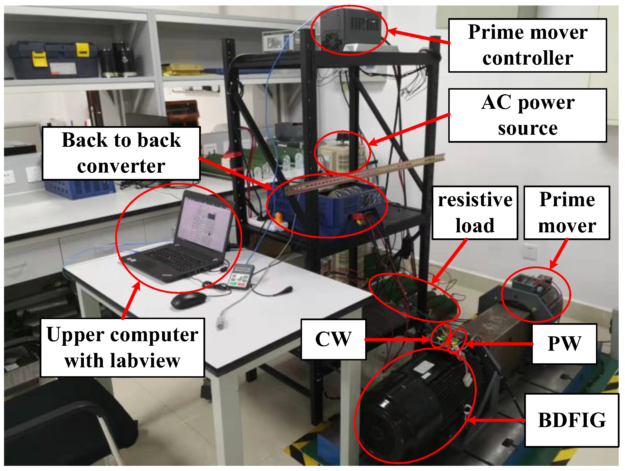
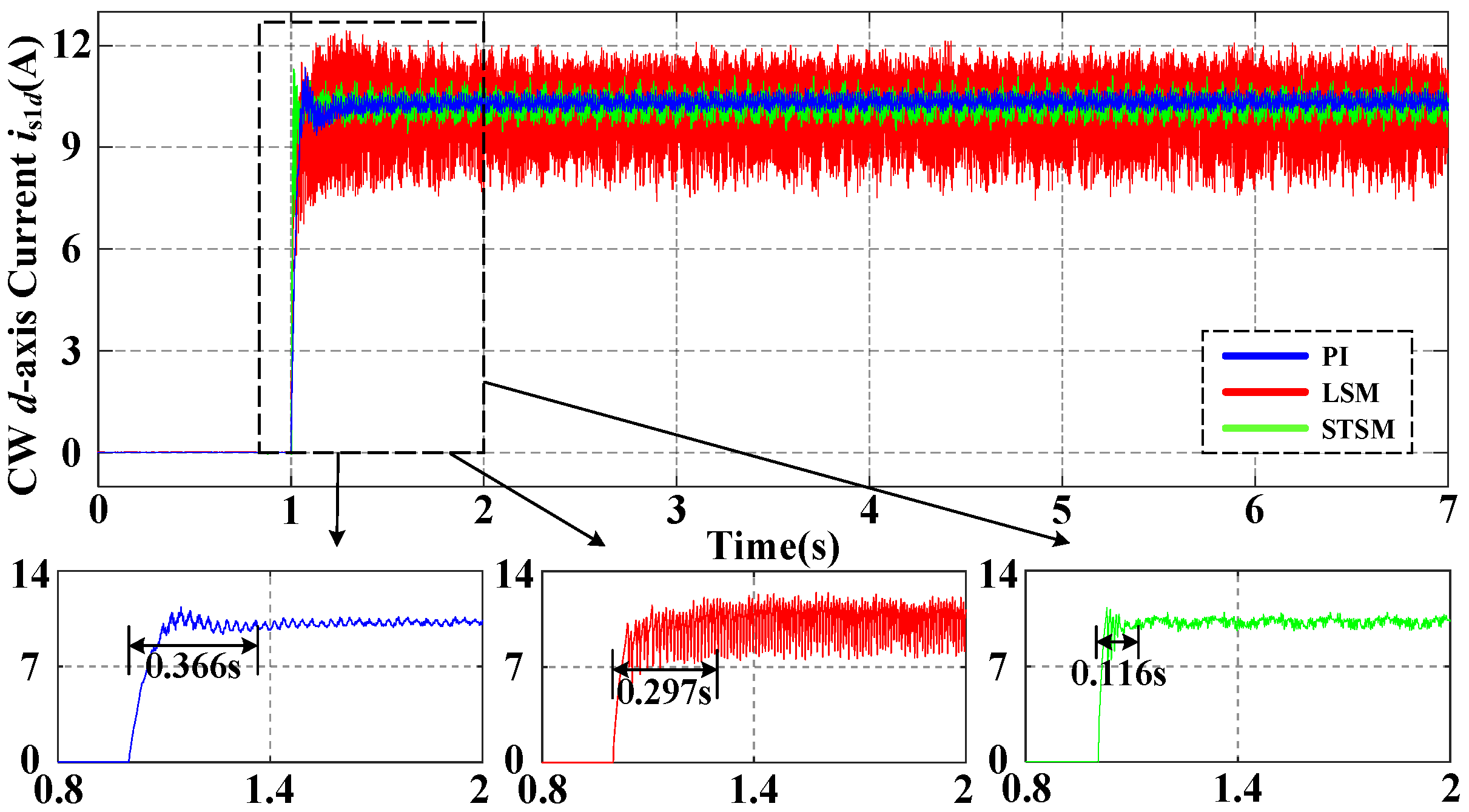
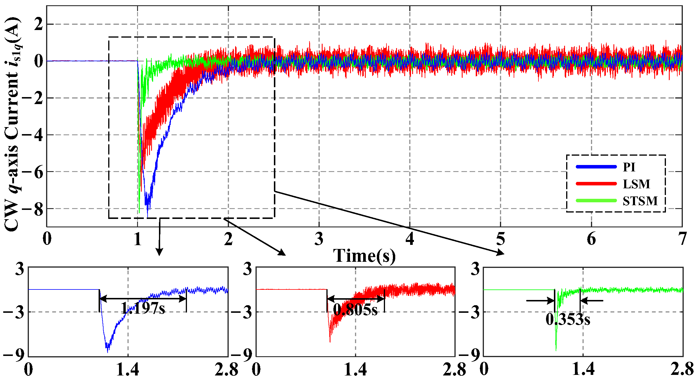
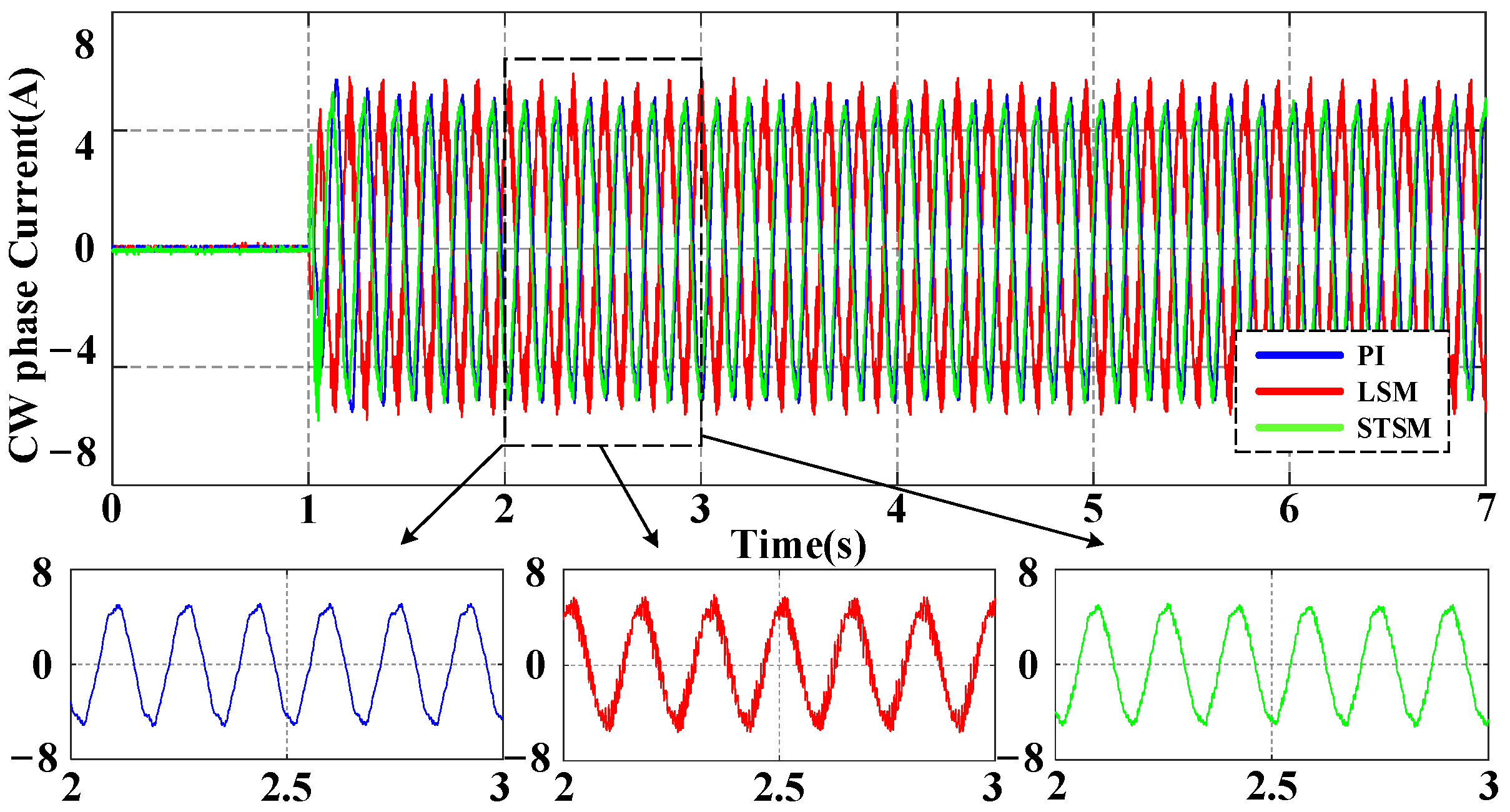
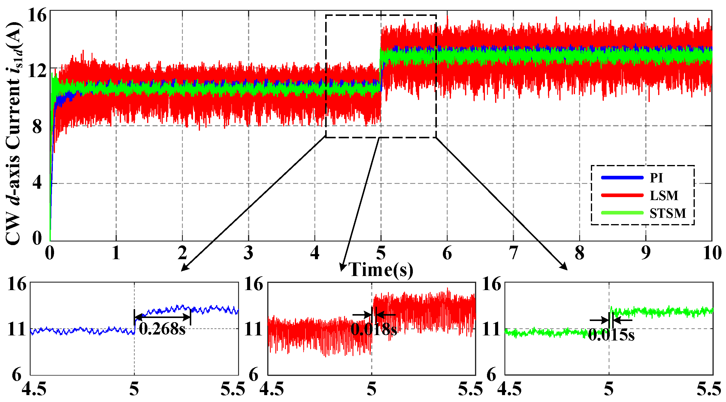
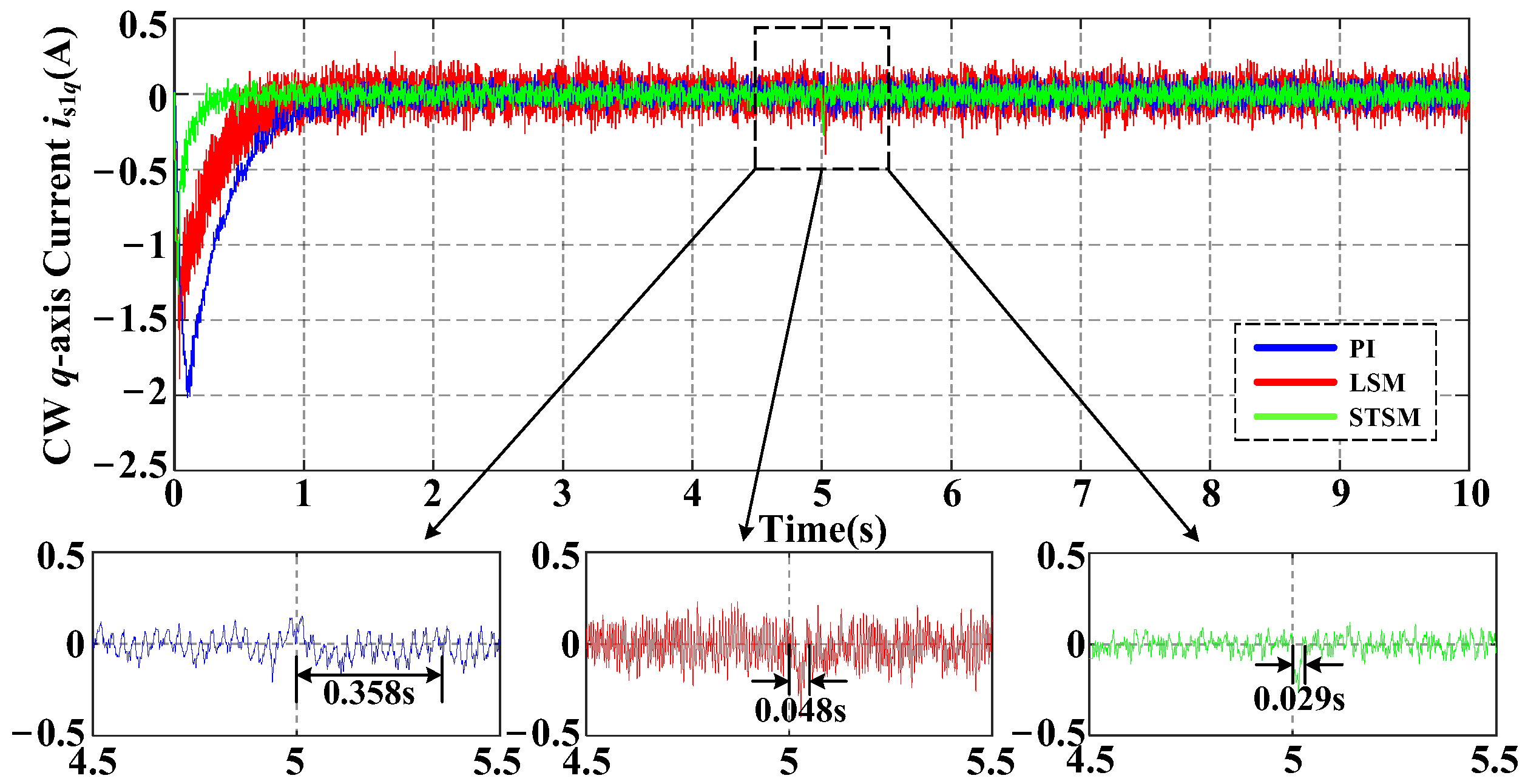
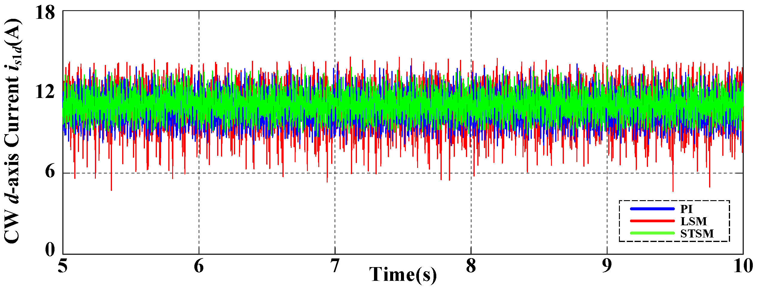
4. Experimental Results

To verify the effectiveness of the controller design method proposed in this study, the control performance of the controller in the actual system is verified. The experiment is based on the BDFIG-based ship shaft independent power system shown in Figure 2. The BDFIG experimental platform includes a 5 kVA brushless doubly-fed motor (Tianjin Tongyu Jiahe Energy Saving Technology Co., Ltd., Tianjin, China) and a 10 kW induction motor (Zhong Dalide Intelligent Transmission Equipment Co., Ltd., Ningbo, China) as the prime mover to drive the BDFIG, as well as a set of four-quadrant inverters based on a TMS320F28335 chip (Texas instruments, Dalas, TX, USA), voltage and current sensors (Precision Electronics (Shenzhen) Co., Ltd., Shenzhen, China), and a host computer built by LabView. The communication protocol selects the CAN communication protocol, and the motor sampling frequency is set as 5 kHz. The parameters of the brushless doubly-fed machine on the experimental platform are shown in

Table 1. Experiment parameters.

Parameter	Value	Parameter	Value
Capacity	3 kW	Rr	8.691 Ω
PW pole pairs	1	Rs	4.21 Ω
PW pole pairs	2	Rs1	3.10 Ω
Natural speed	1000 rpm	Ls	1.510 H
Speed range	700–1200 rpm	Ls1	0.8908 H
PW rated voltage	380 V	Lr	2.134 H
PW rated current	4.5 A	Lsr	1.466 H
CW rated voltage	350 V	Ls1r	0.5911 H
CW rated current	8 A	Rotor type	Wound rotor

below.

The startup and loading change conditions were investigated in an experiment. In the experiment, the reference voltage was set at 150 V. To account for uncertainties stemming from aging and temperature variations, the values of R_i and L_i in the control algorithm were adjusted to 120% of their nominal values. The startup experiment results are shown in Figure 3 and Figure 4. The CW d-axis current rising response time with proportional-integral (PI), linear sliding mode (LSM), and STSM controllers are 0.366 s, 0.297 s, and 0.116 s, respectively. STSM exhibits a quicker dynamic response. The same conclusion can be drawn from experimental data on the current of the q-axis.

Figure 5 and Figure 6 show the CW phase current and the effective values of PW line voltage under the starting experiment. In Figure 5 and Figure 6, the proposed STSM has smaller steady-state fluctuations compared to LSM and PI, but it has a faster dynamic response. These experimental results demonstrate that the proposed STSM controller exhibits a quick dynamic response and strong robustness against the uncertainties caused by parameter perturbation.

The experiment results under loading condition are shown in Figure 7 and Figure 8. In Figure 7 and Figure 8, the stability time of the d-axis current and the recovery time of the q-axis current with STSMC are both smaller than PI controller. The robustness against the uncertainties with proposed STSM is proven by the results of the loading experiment.

To verify the robustness of the proposed method under parameter perturbation. The values of R_i and L_i in the control algorithm are adjusted to 160% of the nominal value, and the experimental results are shown in Figure 9 and Figure 10. The d-axis current response and q-axis current response of the CW side under the three control methods all show that the CW current response under the STSM control method have smaller ripples.

Compared with the existing methods [12,15,24,25], the steady-state time and accuracy are shown in

Table 2. Comparison of existing methods.

Name	Convergence Time	Steady-State Accuracy	Chattering
ADRC	4.50 s	1.2 × 10−2	free
ISMC	3.15 s	1.12 × 10−4	exists
TSMC	2.31 s	1 × 10−2	exists
Standard STSMC	3.85 s	4 × 10−2	free
Improved STSMC	0.83 s	3 × 10−6	free

.

It can be seen in Table 2 that the mismatched uncertainties lead to a reduction in the steady-state accuracy of active disturbance rejection control (ADRC), ISMC, TSMC, and standard STSM control. The improved STSM control method can overcome the mismatched uncertainties, thus achieving the highest accuracy among the methods. For the dynamic performance, the proposed method has the fastest dynamic response, while other methods compromise their response speed to guarantee the steady-state accuracy. The control of ISMC and TSMC has chattering, while the control signals using standard STSM and improved STSM are smooth without chattering. In summary, the proposed improved STSM control represent better control performance than the other methods in terms of chattering suppression, dynamic response, and especially steady-state accuracy under mismatched uncertainties.

5. Conclusions

In this study, an improved STSM controller of the BDFIG for standalone ship shaft power generation systems is designed. The mechanism of parameter perturbations is analyzed, and the mismatched uncertain model of BDFIG is established to improve the modelling accuracy. The proposed improved STSM method uses virtual control technology to compensate for the mismatched uncertainties, so that the PW voltage error can converge to the equilibrium point rather than the neighborhood, and the steady-state accuracy of the system is enhanced. Meanwhile, the improved STSM method brings excellent dynamic performance and eliminates chattering, which improves the rapidity and robustness of the standalone ship shaft power generation systems. The excellent performance of the proposed method in voltage control is verified by experiments. However, this study has the following two limitations:

(1)

Real-world component selection and constraints: idealized components are assumed in the theoretical controller design and experimental validation. However, practical applications face challenges related to the component’s selection, bandwidth limitations, noise sensitivity, the cost-effectiveness of high-bandwidth sensors, and marine operating conditions (vibration, high temperature, high humidity).

(2)

Computational complexity: the improved STSM method, while effective, has high computational requirements, especially for the existing control chip of the ships.

Future research will focus on addressing these limitations:

(1)

Hardware implementation: to verify the controller’s effectiveness, rigorous tests simulating real marine environments and using commercial chip will be conducted in our future studies.

(2)

Algorithm optimization: methods reducing the computational burden of the proposed improved STSM will be explored in our future research.

References

1. Liu, Y.; Hussien, M.G.; Xu, W.; Shao, S.; Rashad, E.M. Recent Advances of Control Technologies for Brushless Doubly-Fed Generators. IEEE Access 2021, 9, 123324–123347. [Google Scholar] [CrossRef]
2. Knight, A.M.; Betz, R.E.; Dorrell, D.G. Design and Analysis of Brushless Doubly Fed Reluctance Machines. IEEE Trans. Ind. Appl. 2021, 49, 50–58. [Google Scholar] [CrossRef]
3. Abad, G.; Lopez, J.; Rodriguez, M.; Marroyo, L.; Iwanski, G. Doubly Fed Induction Machine: Modeling and Control for Wind Energy Generation; John Wiley & Sons: Hoboken, NJ, USA, 2011. [Google Scholar]
4. Boldea, I.; Tutelea, L.N.; Wu, C.; Blaabjerg, F.; Liu, Y.; Hussien, M.G.; Xu, W. Fractional kVA Rating PWM Converter Doubly Fed Variable Speed Electric Generator Systems: An Overview in 2020. IEEE Access 2021, 9, 117957–117968. [Google Scholar] [CrossRef]
5. Xu, W.; Dong, D.; Liu, Y.; Yu, K.; Gao, J. Improved sensorless phase control of stand-alone brushless doubly-fed machine under unbalanced loads for ship shaft power generation. IEEE Trans. Energy Convers. 2018, 33, 2229–2239. [Google Scholar] [CrossRef]
6. Vadim, K.; Goncharov, N. Problem statement on the vessel braking within ice channel, Transportation Safety and Environment. Transp. Saf. Environ. 2021, 3, 50–56. [Google Scholar]
7. Chen, X.; Wei, C.; Xin, Z.; Zhao, J.; Xian, J. Ship Detection under Low-Visibility Weather Interference via an Ensemble Generative Adversarial Network. J. Mar. Sci. Eng. 2023, 11, 2065. [Google Scholar] [CrossRef]
8. Shao, S.; Abdi, E.; Barati, F.; McMahon, R. Stator-flux-oriented vector control for brushless doubly fed induction generator. IEEE Trans. Ind. Electron. 2009, 56, 4220–4228. [Google Scholar] [CrossRef]
9. Hussien, M.G.; Liu, Y.; Xu, W.; Junejo, A.K.; Allam, S.M. Improved MRAS Rotor Position Observer Based on Control Winding Power Factor for Stand-Alone Brushless Doubly-Fed Induction Generators. IEEE Trans. Energy Convers. 2022, 37, 707–717. [Google Scholar] [CrossRef]
10. Poza, J.; Oyarbide, E.; Sarasola, I.; Rodriguez, M. Vector control design and experimental evaluation for the brushless doubly fed machine. IET Electr. Power Appl. 2009, 3, 247–256. [Google Scholar] [CrossRef]
11. Boudjema, Z.; Taleb, R.; Djeriri, Y.; Yahdou, A. A novel direct torque control using second order continuous sliding mode of a doubly fed induction generator for a wind energy conversion system. Turk. J. Electr. Eng. Comput. Sci. 2017, 25, 965–975. [Google Scholar] [CrossRef]
12. Sadeghi, R.; Madani, S.M.; Ataei, M.; Kashkooli, M.R.A.; Ademi, S. Super-twisting sliding mode direct power control of a brushless doubly fed induction generator. IEEE Trans. Ind. Electron. 2018, 65, 9147–9156. [Google Scholar] [CrossRef]
13. Yan, X.; Cheng, M. A robustness-improved control method based on ST-SMC for cascaded brushless doubly fed induction generator. IEEE Trans. Ind. Electron. 2020, 68, 7061–7071. [Google Scholar] [CrossRef]
14. Sankhwar, P. Application of Permanent Magnet Synchronous Motor for Electric Vehicle. Indian J. Des. Eng. 2024, 4, 1–6. [Google Scholar] [CrossRef]
15. Guo, H.; Zhang, X. Extended State Observer (ESO) Based Control Strategy with Parameter Optimization for Brushless Doubly-fed Machine. In Proceedings of the 2017 2nd International Conference on Automatic Control and Information Engineering (ICACIE 2017), Hong Kong, China, 26–28 August 2017. [Google Scholar]
16. Utkin, V.; Poznyak, A.; Orlov, Y.; Polyakov, A. Conventional and high order sliding mode control. J. Frankl. Inst. 2020, 357, 10244–10261. [Google Scholar] [CrossRef]
17. Pan, Y.; Yang, C.; Pan, L.; Yu, H. Integral sliding mode control: Performance, modification, and improvement. IEEE Trans. Ind. Inform. 2017, 14, 3087–3096. [Google Scholar] [CrossRef]
18. Feng, Y.; Yu, X.; Han, F. On nonsingular terminal sliding-mode control of nonlinear systems. Automatica 2013, 49, 1715–1722. [Google Scholar] [CrossRef]
19. Feng, Y.; Han, F.; Yu, X. Chattering free full-order sliding-mode control. Automatica 2014, 50, 1310–1314. [Google Scholar] [CrossRef]
20. Levant, A. Sliding order and sliding accuracy in sliding mode control. Int. J. Control. 1993, 58, 1247–1263. [Google Scholar] [CrossRef]
21. Levant, A. Chattering analysis. IEEE Trans. Autom. Control. 2010, 55, 1380–1389. [Google Scholar] [CrossRef]
22. Moreno, J.A.; Osorio, M. Strict Lyapunov functions for the super-twisting algorithm. IEEE Trans. Autom. Control. 2012, 57, 1035–1040. [Google Scholar] [CrossRef]
23. Manzanilla, A.; Ibarra, E.; Salazar, S.; Zamora, Á.E.; Lozano, R.; Muñoz, F. Super-twisting integral sliding mode control for trajectory tracking of an Unmanned Underwater Vehicle. Ocean. Eng. 2021, 234, 109164. [Google Scholar] [CrossRef]
24. Yang, X.; Qin, Y.; Zhan, J.; Li, Y.; Hao, S.; Fu, Z. Direct Power Control of BDFRG Based on Novel Integral Sliding Mode Control. Recent Adv. Electr. Electron. Eng. 2024, 17, 1–16. [Google Scholar] [CrossRef]
25. Zhan, Y.; Guo, Y.; Zhu, J. Terminal sliding mode speed controller based on vector control for brushless doubly fed machine. In Proceedings of the 2011 International Conference on Applied Superconductivity and Electromagnetic Devices, Sydney, Australia, 14–16 December 2011. [Google Scholar]
Figure 1. The control block diagram of the BDFIG-based independent power generation system.
Jmse 13 01358 g001
Figure 2. Laboratory equipment of the BDFIG ship shaft independent power system.
Jmse 13 01358 g002
Figure 3. Experimental results of the CW d-axis current with PI, LSM, and STSM under startup conditions.
Jmse 13 01358 g003
Figure 4. Experimental results of the CW q-axis current with PI, LSM, and STSM under startup conditions.
Jmse 13 01358 g004
Figure 5. Experimental results of the CW phase current with PI, LSM and STSM under startup conditions.
Jmse 13 01358 g005
Figure 6. Experimental results of the RMS of the PW line voltage with PI, LSM and STSM under startup conditions.
Jmse 13 01358 g006
Figure 7. Experimental results of the CW d-axis current with PI, LSM, and STSM under loading conditions.
Jmse 13 01358 g007
Figure 8. Experimental results of the CW q-axis current with PI, LSM and STSM under loading conditions.
Jmse 13 01358 g008
Figure 9. Experimental results of the CW d-axis current with PI, LSM, and STSM under 150% parameter perturbation.
Jmse 13 01358 g009
Figure 10. Experimental results of the CW q-axis current with PI, LSM and STSM under 150% parameter perturbation.
Jmse 13 01358 g010