Autonomous Tracking of Steel Lazy Wave Risers Using a Hybrid Vision–Acoustic AUV Framework

Abstract

Steel lazy wave risers (SLWRs) are critical in offshore hydrocarbon transport for linking subsea wells to floating production facilities in deep-water environments. The incorporation of buoyancy modules reduces curvature-induced stress concentrations in the touchdown zone (TDZ); however, extended operational exposure under cyclic environmental and operational loads results in repeated seabed contact. This repeated interaction modifies the seabed soil over time, gradually forming a trench and altering the riser configuration, which significantly impacts stress patterns and contributes to fatigue degradation. Accurately reconstructing the riser’s evolving profile in the TDZ is essential for reliable fatigue life estimation and structural integrity evaluation. This study proposes a simulation-based framework for the autonomous tracking of SLWRs using a fin-actuated autonomous underwater vehicle (AUV) equipped with a monocular camera and multibeam echosounder. By fusing visual and acoustic data, the system continuously estimates the AUV’s relative position concerning the riser. A dedicated image processing pipeline, comprising bilateral filtering, edge detection, Hough transform, and K-means clustering, facilitates the extraction of the riser’s centerline and measures its displacement from nearby objects and seabed variations. The framework was developed and validated in the underwater unmanned vehicle (UUV) Simulator, a high-fidelity underwater robotics and pipeline inspection environment. Simulated scenarios included the riser’s dynamic lateral and vertical oscillations, in which the system demonstrated robust performance in capturing complex three-dimensional trajectories. The resulting riser profiles can be integrated into numerical models incorporating riser–soil interaction and non-linear hysteretic behavior, ultimately enhancing fatigue prediction accuracy and informing long-term infrastructure maintenance strategies.

1. Introduction

Offshore oil and gas exploration has increasingly advanced into deeper and ultra-deep waters. Riser systems, essential for connecting subsea production units to floating platforms, enable the safe and efficient transfer of oil and gas. Several types of risers have been developed to accommodate the demands of different floating platform designs. 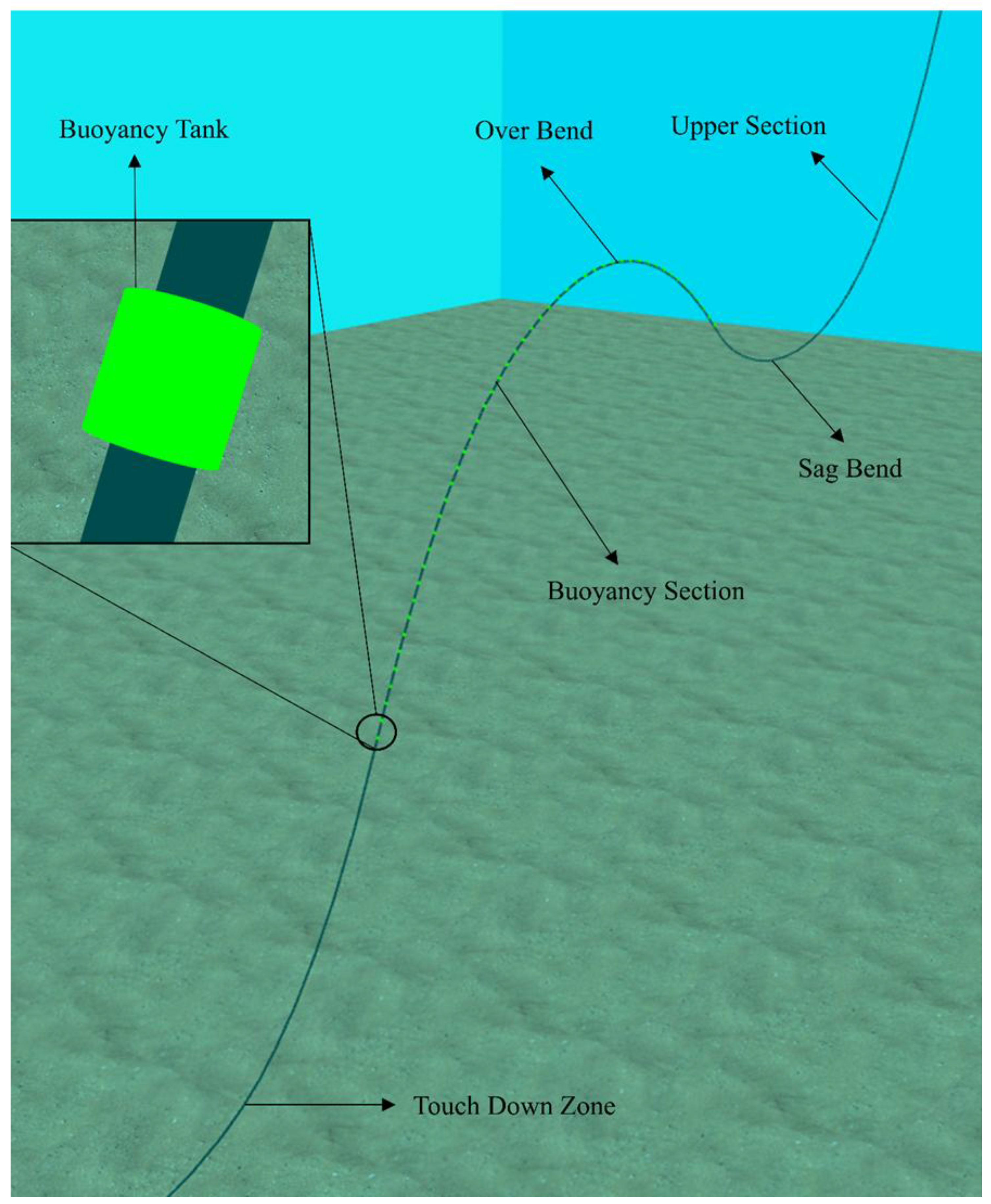Each system comes with unique advantages and constraints [1]. SLWRs have become increasingly popular in deep-water projects due to their ability to address critical challenges associated with steel catenary risers (SCRs). By incorporating buoyancy modules along the mid-section of the riser, SLWRs effectively reduce the fatigue issues prevalent in SCRs, particularly in the TDZ, where frequent interactions with the seabed cause significant fatigue. While SCRs were traditionally favored for their simplicity and cost-effectiveness in installation, their applications were limited in harsher environments due to these fatigue-related vulnerabilities [2]. In particular, the fatigue behavior of risers in the touchdown zone is influenced not only by platform dynamics and ocean currents but also by long-term riser–soil interaction. Under cyclic loading, repeated contact between the riser and seabed leads to soil deformation and trench development, often reaching depths of 3–5 riser diameters over time. These geometric changes can profoundly alter stress distributions along the riser, making accurate reconstruction of its evolving profile critical for fatigue life estimation and structural integrity assessments. Deep-sea operations such as riser monitoring and trench analysis are impossible for humans to perform due to the immense pressure and harsh conditions. This is where AUVs play a transformative role. Unlike traditional underwater vehicles, AUVs operate without the need for cumbersome tethers or umbilical cables, giving them greater mobility and the ability to work for extended periods in remote and deep-sea areas. Their self-driving capabilities, when enhanced with artificial intelligence (AI) for decision-making, push the boundaries of autonomy, allowing them to handle complex tasks more efficiently. By reducing the need for human intervention in hazardous environments, AUVs offer a safer, more cost-effective, and environmentally friendly solution for underwater operations [3,4,5]. AUVs can be equipped with a variety of sensors tailored for specific underwater operations. Multibeam echo sounders (MBES) are used for mapping and detecting small objects, while side-scan sonar (SSS) excels in monitoring pipelines and conducting seabed surveys. Optical cameras, often paired with artificial lights for deeper conditions, enable visual tracking and simultaneous localization and mapping (SLAM) [6,7]. In this context, AUVs equipped with vision and acoustic sensors offer a promising solution for autonomous riser tracking. By accurately estimating their position relative to the riser and surrounding features, these systems can extract detailed three-dimensional profiles, particularly within the TDZ. When deployed in simulated environments such as the UUV Simulator, these frameworks can be rigorously tested under dynamic seabed and riser conditions. The resulting spatial data not only enhances AUV control strategies but also provides valuable input for fatigue modeling that accounts for trench formation and non-linear riser–soil interaction effects.

In recent years, various studies have been conducted in the field of autonomous underwater cable and pipeline tracking using different sensing and optimization techniques. Feng et al. [8] introduced a non-myopic receding-horizon optimization (RHO) strategy for optimizing imaging quality to track underwater cables using AUVs equipped with side-scan sonar (SSS). They incorporate long short-term memory (LSTM) networks to predict cable states, minimize AUV motion instability, and enhance sonar imaging quality. The study by Zhang et al. [9] proposed a vision-based framework for detecting and tracking underwater pipelines using a monocular CCD camera. The method involved image preprocessing with the Sobel operation [10] and Hough transform [11] for edge detection, followed by Kalman filtering [12] to predict pipeline positions in subsequent frames. The system was evaluated in a 50 m × 30 m × 10 m tank with five 6-meter-long sewer pipes as simulated pipelines. Zhang, T. et al. [13] proposed an online framework for tracking underwater moving targets using forward-looking sonar (FLS) images, leveraging a Gaussian particle filter (GPF) for multi-target tracking in cluttered environments. The framework incorporated modified median filtering and region-growing segmentation to enhance image processing, while feature selection was optimized using a generalized regression neural network (GRNN) combined with sequential forward and backward selection. Abu, A., & Diamant, R. [14] presented a SLAM-based approach for AUV localization using optical and synthetic aperture sonar (SAS) image matching. The method models SAS-detected objects as hidden Markov model (HMM) states and employs a constrained Viterbi algorithm to determine the AUV’s position based on similarity rankings of optical camera observations. Experiments with real SAS and optical data in simulated environments demonstrated high localization accuracy and robustness against image noise. The study also analyzed sensitivity to the number of detected objects and AUV heading accuracy, with future work aiming to integrate seabed feature extraction. Petillot, Y. et al. [15] introduced two techniques for pipeline tracking using multibeam echo sounders and side-scan sonar, employing a model-based Bayesian framework for robust detection. The method involves segmenting noisy side-scan sonar images with an unsupervised Markov random field model and detecting pipe-like shadows using adaptive filters. Line fitting is performed using a least median squared algorithm followed by least-squares refinement for robust results.

Akram, W., & Casavola, A. [16] proposed a visual control scheme for tracking underwater pipelines using an AUV-mounted downward-looking camera. The method processes robot operating system (ROS)-collected images with OpenCV to segment the pipeline based on HSV (hue, saturation, value) values and recover its coordinates, enabling the AUV to follow the pipeline’s longitudinal axis. The system integrates image processing, coordinate recovery, and proportional integral derivative (PID) control, tested using a modified UUV Simulator in ROS and Gazebo. Alla, D. N. V. et al. [17] explored underwater object detection in shallow waters using a transfer learning-based You Only Look Once YOLOv4 model enhanced with underwater image processing techniques. The methodology involved data augmentation, including cropping and flipping, and applied dehazing and deblurring methods to improve image quality. Hu et al. [18] demonstrated a vision-based robotic fish capable of autonomously tracking dynamic targets underwater. Drawing inspiration from the stability and agility of the boxfish, the system used a digital camera alongside an improved continuously adaptive mean shift (Camshift) algorithm to maintain visual focus on the target. The algorithm relied on the target’s color histogram in the YCrCb color space, specifically leveraging the Cr and Cb components for enhanced robustness under varying lighting conditions. This approach minimized computational demands while ensuring adaptive tracking. As the target moved within the image or varied in distance, the algorithm dynamically adjusted the search window, allowing the robotic fish to reposition itself and sustain consistent tracking performance.

Yu, J. et al. [19] addressed this by developing a vision-based system with a camera stabilizer and a deep reinforcement learning (DRL) controller. The system integrates a kernelized correlation filter (KCF) for efficient target detection and uses proportional–derivative (PD) control to stabilize images by compensating for disturbances. The Deep Deterministic Policy Gradient (DDPG)-based deep reinforcement learning (DRL) controller manages continuous state–action spaces to optimize motion parameters.

Da Silva et al. [20] employed YOLO and classical image processing techniques, such as Canny edge detection and Hough transform, to track unburied pipelines by identifying and extracting pipeline reference lines. The method was validated through simulations using PX4 software-in-the-loop (SITL) with ROS and Gazebo and further confirmed by real-world tests, achieving 72% accuracy in pipe detection and a 0.0111 m mean squared error in path tracking. To enhance underwater inspection capabilities, Fan, J. et al. [21] developed a system for subsea pipeline tracking and 3D reconstruction using structured light vision (SLV). The system, integrated into the BlueROV underwater vehicle, combines SLV sensors, dual-line lasers, a camera, and a Doppler velocity log (DVL) to achieve precise positioning and tracking. Experimental validation was conducted in a controlled pool environment measuring 5 × 4 × 1.5 m, using a pipeline model with a 1.4 m length, a 7.5 cm diameter, and a 45-degree bend. Bobkov et al. 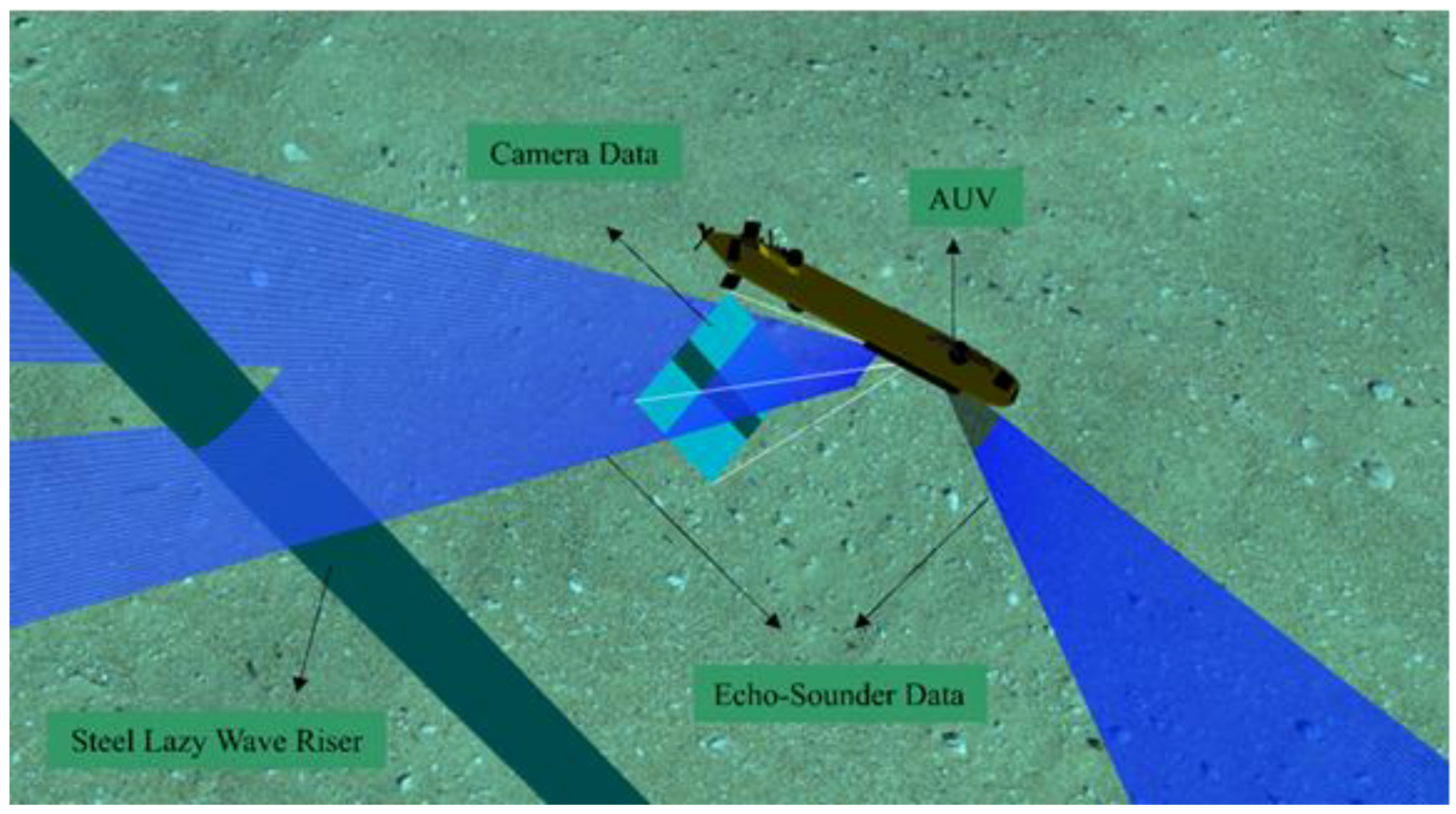[22] focused on improving the inspection of underwater pipelines (UPs) using AUVs by leveraging stereo image data for enhanced accuracy. The proposed method includes an algorithm to calculate the 3D centerline of visible pipeline segments by combining 2D and 3D video data. Key features include using modified Hough’s algorithm for efficient pipeline contour construction, a voting mechanism to select the most reliable solution, and techniques to resume tracking after temporary visibility loss, such as pipelines covered by sediments. The approach allows precise determination of the relative positions of the AUV and the pipeline, enabling both tracking and contact-based inspection operations. In this paper, we propose a methodology for detecting the boundaries of a steel lazy wave riser using stereo camera data, enabling the AUV to align its trajectory with the riser’s centerline. The system ensures a predefined standoff distance by utilizing a multibeam echosounder for precise distance measurement. A secondary echosounder mounted at the front of the AUV aids in collision avoidance, particularly with the upward sections of the riser. This approach enables the AUV to navigate past the buoyancy modules installed along the riser, ensuring safe traversal while maintaining proximity to the riser’s structure from the hang-off point to the riser’s termination point.

Despite the diverse advancements in vision-based tracking, sonar-aided localization, and deep-learning-enhanced detection techniques, most existing methods have focused on straight pipelines or low-complexity trajectories, often in controlled or shallow-water environments. There remains a clear gap in tracking risers with dynamic, three-dimensional geometries, such as SLWRs, particularly in deep-sea settings where seabed interaction introduces additional challenges. This work presents a unified tracking framework that combines stereo image-based boundary detection with acoustic range measurements to guide a fin-actuated AUV along the riser’s centerline. The system ensures an adaptive standoff distance, enables safe passage around buoyancy modules, and provides spatial data that can support fatigue modeling by capturing the riser’s full three-dimensional shape from hang-off to termination.

2. Missions and Framework

2.1. System Architecture

The autonomous underwater system is based on the ECA Group’s A9 fin-based autonomous AUV, designed for high-precision subsea missions. This AUV is equipped with a suite of sensors to facilitate navigation and environmental interaction. At both the front and rear sections, multibeam echosounders are installed, each offering a 30-degree field of view and comprising 60 beams. These sensors are pivotal for accurate distance measurements and practical obstacle avoidance. By emitting multiple beams across a wide angle, they generate dense depth information, allowing the AUV to estimate its distance from the riser with high precision. This supports safe navigation and ensures robust performance even when visual input is degraded due to turbidity or poor lighting. Complementing these is an optical camera mounted at the front, featuring a 30-degree field of view and a resolution of 400 × 300 pixels, which is utilized for visual tracking tasks.

The operational environment is simulated to mirror realistic subsea conditions, encompassing a depth of 800 m, dynamic sea surface interactions, and the presence of a steel lazy wave riser, as depicted in Figure 1. The simulation leverages UUV Simulator [23], an open-source platform built upon the ROS and Gazebo. This simulator facilitates the integration and testing of various underwater vehicles and sensors. The AUV’s physical structure and sensor placements are defined using unified robot description format (URDF) files, while the environment is configured through simulation description format (SDF) files [24]. Custom behaviors for actuators and sensors are implemented via C++ plugins, allowing for tailored simulations.

2.2. Riser-Tracking Approach

The primary mission objective is to enable the AUV to autonomously track the profile of a steel lazy wave riser, extending from the hang-off point to its touchdown zone on the seabed. This is achieved through real-time sensor data processing to ascertain the AUV’s relative position concerning the riser, subsequently adjusting its trajectory to maintain alignment.

The riser’s complex geometry is meticulously modeled, including features such as the over-bend near the floating facility, as shown in Figure 2, buoyant sections with yellow buoyancy tanks, the sag bend, and the touchdown zone. Designs are created in SolidWorks (2024) and imported into the simulation environment using appropriate mesh formats. These models are refined using numerical simulations conducted with OrcaFlex, ensuring an accurate representation of the riser’s physical characteristics and behavior under various conditions. Integrating advanced sensor data processing with precise environmental modeling enables the AUV to perform reliable and efficient riser-tracking operations, even in challenging underwater environments.

The profile shows buoyancy tanks, the sag bend, the over-bend upper section, and the path down to the touchdown point on the seabed.

3. Navigation and Path Estimation Strategy

3.1. Sensor Integration and Data Handling

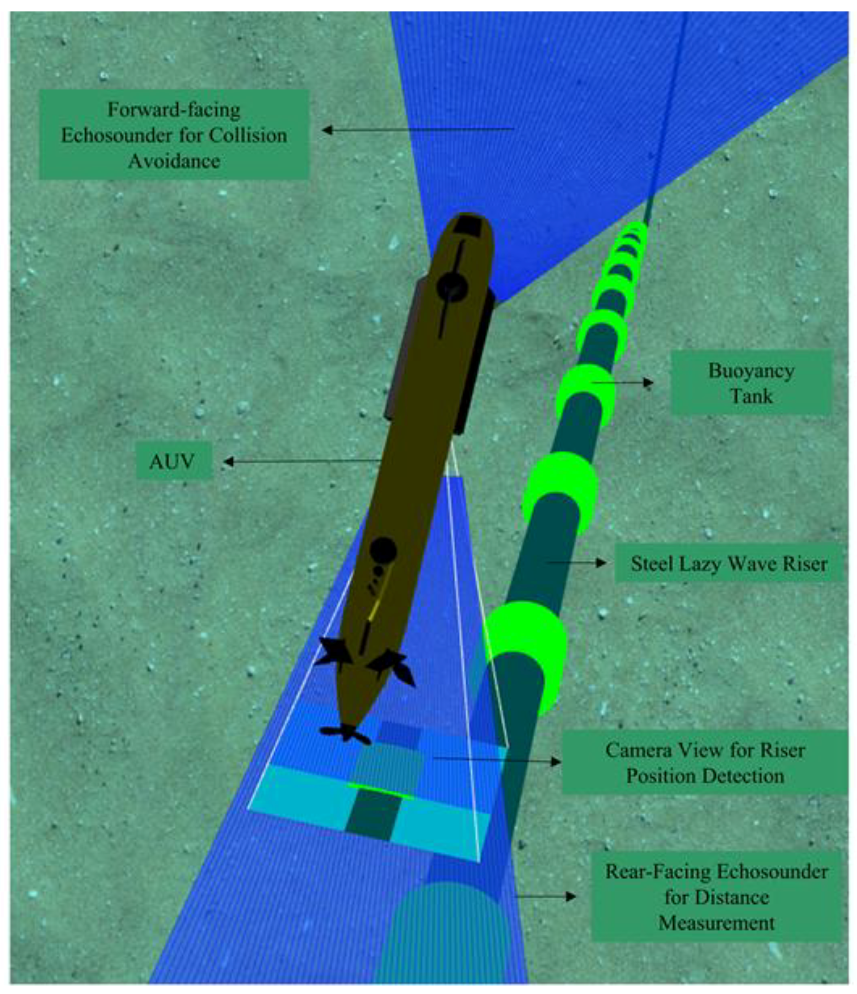
The AUV employs a stereo camera mounted at the front, as depicted in Figure 3, to capture visual data essential for navigation and tracking tasks. The images obtained are transmitted via the cv_bridge library, which facilitates the conversion of ROS image messages into OpenCV-compatible formats, enabling efficient image processing within the ROS framework. This interaction is managed through an ROS Python (rospy) subscriber, which uses the sensor_msgs/Image module to receive image data from the camera sensor.

The riser is visible in the camera’s field of view, with one yellow buoyancy tank along its buoyant section. In parallel, the AUV utilizes multibeam echosounders mounted at both the front and rear, each configured with a 30-degree field of view and comprising 60 beams. These sensors are critical for distance measurement and obstacle avoidance. The sensor_msgs/Range module processes the echosounder inputs, allowing the AUV to maintain a safe and consistent distance from the riser, thereby preventing collisions during forward motion. The visual and acoustic data streams are managed within a Python 2.7 ROS node, ensuring synchronized and efficient handling of sensor information.

3.2. Riser Detection and Tracking Pipeline

The AUV’s ability to accurately detect and track the steel lazy wave riser relies on a robust image processing pipeline designed to operate effectively in challenging underwater conditions. The pipeline initiates with bilateral denoising, which smooths the image while preserving important edges by considering spatial proximity and intensity similarity. This approach effectively reduces underwater noise without distorting critical features, ensuring the clarity of the riser in noisy environments.

Following denoising, the pipeline applies the Canny edge detection algorithm to identify prominent edges by highlighting regions of significant intensity change. This algorithm employs gradient computation, non-maximum suppression, and hysteresis to produce clean, well-defined edges, making the riser’s boundaries more visible. Subsequently, the Hough transform is utilized to detect linear features within the edge-detected image. This method identifies the riser’s straight edges with high precision by transforming edge points into a parameter space, even amidst complex backgrounds.

To further enhance accuracy, K-means clustering is applied to group the detected edge points. This step isolates the riser’s edges from other features, such as seabed structures, and helps define the riser’s centerline by averaging the most significant clusters of edge points. Together, these steps create a robust pipeline capable of accurately identifying and tracking the riser in challenging underwater conditions.

The integration of vision-based data with echosounder measurements enables the AUV to adjust its position in real time, achieving robust and consistent tracking even in noisy underwater environments. By analyzing the shortest range recorded in the echosounder beams, the system calculates the distance between the AUV and the riser, ensuring the AUV maintains a controlled position relative to the riser, supporting accurate tracking and reliable navigation.

4. Tracking Scenario

Building on the sensor processing pipeline described above, the AUV makes real-time trajectory adjustments based on the detected position of the riser in the east–north–up (ENU) coordinate system, where X points east, Y points north, and Z points up or down, which fully defines the robot’s position and rotation. Hydrodynamic forces, derived from Fossen’s mathematical equations [24], are applied to the AUV’s body, taking into account its speed and mechanical specifications. Sensor data determines whether the AUV needs to move left or right (yaw adjustment) or up or down (pitch adjustment).

Commands are sent to the AUV’s actuators, including fins and propellers. These convert angular velocity, yaw, and pitch angle inputs into drag, lift, and thrust forces to maintain the AUV’s position and move toward the desired direction. Since the SLWR follows a non-linear path influenced by wave amplitude and frequency, the AUV’s motion must account for these variations. The desired pitch and yaw angles are computed as a proportion of the deviation from the riser’s centerline and its distance from the AUV. The tracking is performed as a feedback loop, where vision and acoustic sensors continuously provide position updates, the AUV dynamically calculates the required adjustments to maintain its trajectory, and non-linear variations in the riser’s motion are compensated to ensure smooth tracking. This approach ensures precise alignment with the riser’s path, from the hang-off point to its endpoint, enabling thorough inspection and monitoring under varying environmental conditions.

5. Performance Metrics

5.1. Precision and Recall

Precision and recall are fundamental evaluation metrics in classification and detection tasks. Precision measures the proportion of accurate optimistic predictions among all positive predictions, emphasizing minimizing false positives. Recall, also known as sensitivity, measures the proportion of actual positive cases that were correctly identified, focusing on minimizing false negatives. In the context of underwater riser tracking, high precision ensures that detected features correspond accurately to the riser, while high recall ensures that the majority of the riser is successfully captured without omission. Together, they evaluate the system’s ability to detect and track the structure in noisy and complex environments. The mathematical definitions of precision and recall are provided in Equations (1) and (2), respectively, following the formulations outlined by Powers [25].

$$\mathrm{P}\mathrm{r}\mathrm{e}\mathrm{c}\mathrm{i}\mathrm{s}\mathrm{i}\mathrm{o}\mathrm{n}={\displaystyle \frac{\mathrm{T}\mathrm{r}\mathrm{u}\mathrm{e} \mathrm{P}\mathrm{o}\mathrm{s}\mathrm{i}\mathrm{t}\mathrm{i}\mathrm{v}\mathrm{e}}{\mathrm{T}\mathrm{r}\mathrm{u}\mathrm{e} \mathrm{P}\mathrm{o}\mathrm{s}\mathrm{i}\mathrm{t}\mathrm{v}\mathrm{e}+\mathrm{F}\mathrm{a}\mathrm{l}\mathrm{s}\mathrm{e} \mathrm{P}\mathrm{o}\mathrm{s}\mathrm{i}\mathrm{t}\mathrm{i}\mathrm{v}\mathrm{e}}}$$

(1)

$$\mathrm{R}\mathrm{e}\mathrm{c}\mathrm{a}\mathrm{l}\mathrm{l}={\displaystyle \frac{\mathrm{T}\mathrm{r}\mathrm{u}\mathrm{e} \mathrm{P}\mathrm{o}\mathrm{s}\mathrm{i}\mathrm{t}\mathrm{i}\mathrm{v}\mathrm{e}}{\mathrm{T}\mathrm{r}\mathrm{u}\mathrm{e} \mathrm{P}\mathrm{o}\mathrm{s}\mathrm{i}\mathrm{t}\mathrm{v}\mathrm{e}+\mathrm{F}\mathrm{a}\mathrm{l}\mathrm{s}\mathrm{e} \mathrm{N}\mathrm{e}\mathrm{g}\mathrm{a}\mathrm{t}\mathrm{i}\mathrm{v}\mathrm{e}}}$$

(2)

5.2. F1 Score

The F1 score combines precision and recall into a single harmonic mean to provide a balanced measure of detection performance. It is particularly advantageous when dealing with imbalanced datasets, as is common in underwater environments where the riser occupies a small portion of the field of view. A high F1 score indicates that the model maintains a good trade-off between identifying relevant features and avoiding false detections. In riser-tracking scenarios, both false positives and false negatives can have critical operational impacts, making the F1 score an essential evaluation criterion. The F1 score is computed as shown in Equation (3), based on the definitions of precision and recall [25].

$$\mathrm{F}1 \mathrm{S}\mathrm{c}\mathrm{o}\mathrm{r}\mathrm{e}=2\times {\displaystyle \frac{\mathrm{P}\mathrm{r}\mathrm{e}\mathrm{c}\mathrm{i}\mathrm{s}\mathrm{i}\mathrm{o}\mathrm{n}\times \mathrm{R}\mathrm{e}\mathrm{c}\mathrm{a}\mathrm{l}\mathrm{l}}{\mathrm{P}\mathrm{r}\mathrm{e}\mathrm{c}\mathrm{i}\mathrm{s}\mathrm{i}\mathrm{o}\mathrm{n}+\mathrm{R}\mathrm{e}\mathrm{c}\mathrm{a}\mathrm{l}\mathrm{l}}}$$

(3)

5.3. IoU and Dice Coefficient

Intersection over union (IoU) and Dice Coefficient are two widely adopted metrics for evaluating the spatial accuracy of feature localization, particularly in segmentation tasks. In this context, the prediction area refers to the region identified by the algorithm as the riser’s edge; the ground truth area is the manually labeled true riser edge; the area of overlap is the intersection between the predicted and true regions; and the area of union is the total combined area of both predicted and ground truth regions. IoU measures the overlap between the predicted region and the ground truth relative to their union, offering a strict assessment of localization performance. Dice Coefficient, while conceptually similar, emphasizes the overlapping region more strongly and tends to be more sensitive to small structures, making it particularly effective for narrow objects such as underwater risers. Both metrics are crucial for assessing the accuracy and reliability of the AUV’s perception system in subsea environments. Their mathematical formulations are provided in Equations (4) and (5), respectively, based on definitions commonly used in image segmentation literature [25].

$$\mathrm{I}\mathrm{o}\mathrm{U}={\displaystyle \frac{\mathrm{A}\mathrm{r}\mathrm{e}\mathrm{a} \mathrm{o}\mathrm{f} \mathrm{O}\mathrm{v}\mathrm{e}\mathrm{r}\mathrm{l}\mathrm{a}\mathrm{p}}{\mathrm{A}\mathrm{r}\mathrm{e}\mathrm{a} \mathrm{o}\mathrm{f} \mathrm{U}\mathrm{n}\mathrm{i}\mathrm{o}\mathrm{n}}}$$

(4)

$$\mathrm{D}\mathrm{i}\mathrm{c}\mathrm{e}={\displaystyle \frac{2\times \mathrm{A}\mathrm{r}\mathrm{e}\mathrm{a} \mathrm{o}\mathrm{f} \mathrm{O}\mathrm{v}\mathrm{e}\mathrm{r}\mathrm{l}\mathrm{a}\mathrm{p}}{\mathrm{P}\mathrm{r}\mathrm{e}\mathrm{d}\mathrm{i}\mathrm{c}\mathrm{t}\mathrm{i}\mathrm{o}\mathrm{n} \mathrm{A}\mathrm{r}\mathrm{e}\mathrm{a}+\mathrm{G}\mathrm{r}\mathrm{o}\mathrm{u}\mathrm{n}\mathrm{d} \mathrm{T}\mathrm{r}\mathrm{u}\mathrm{t}\mathrm{h} \mathrm{A}\mathrm{r}\mathrm{e}\mathrm{a}}}$$

(5)

6. Results and Discussion

6.1. Stereo Vision and Centerline Extraction

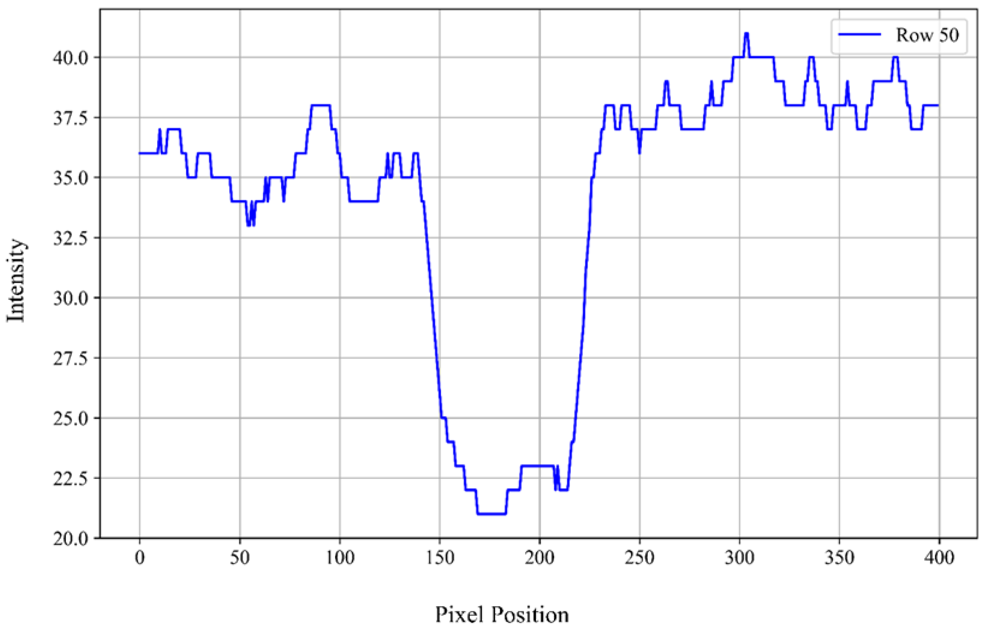
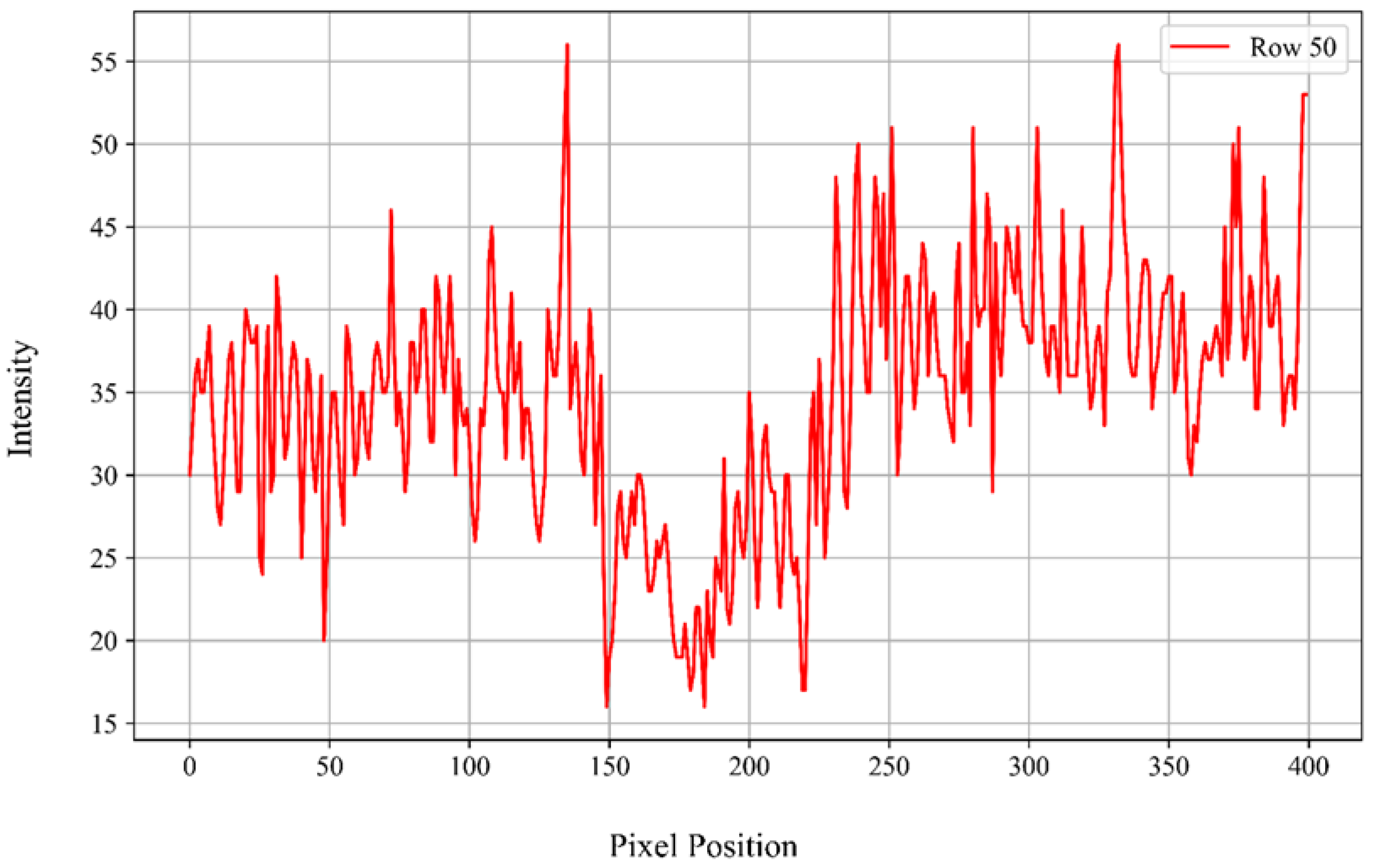
In this pipeline, the process begins with the noisy image undergoing bilateral denoising, a highly effective technique that reduces noise while preserving sharp edges, an essential feature for our task. As illustrated in Figure 4, the intensity profile along the central row (row 50) of the original noisy grayscale image reveals significantly high-frequency variations due to noise. This profile, spanning pixels 0 to 400, exhibits fluctuating intensity levels without a distinct boundary indicating the presence of the riser.

Specifically, from pixel 0 to approximately pixel 150, the intensity values oscillate between 30 and 40, reflecting a noisy background. Between pixels 150 and 250, corresponding to the approximate location of the riser, the intensity levels decrease to a range of 17 to 35, indicating a darker region. Beyond pixel 250 up to pixel 400, the intensity values rise again, fluctuating between 30 and 50, similar to the initial background levels.

This continuous fluctuation across the entire row underscores the challenge in distinguishing the riser from the background based solely on raw intensity values. The absence of a clear intensity demarcation necessitates applying advanced image processing techniques, such as bilateral filtering and edge detection algorithms, to enhance feature extraction and improve the accuracy of riser detection in noisy underwater environments. In contrast, Figure 5 shows the same row after applying the bilateral filter, which significantly smooths the intensity profile along row 50 of the grayscale image. Post-filtering, the intensity values from pixel 0 to 150 stabilize within the 32–37 range, exhibiting reduced fluctuations compared to the original noisy profile. In the riser region (pixels 150–250), intensities further decrease to a narrow band of 21–23, indicating enhanced contrast and clearer delineation of the riser’s boundaries. Beyond pixel 250 up to 400, the intensity values modestly increase, ranging between 35 and 40, yet maintain a smooth transition without abrupt variations. Overall, the bilateral filter effectively suppresses noise-induced fluctuations across the entire row while preserving critical edge information, facilitating more accurate and reliable riser detection in challenging underwater imaging conditions.

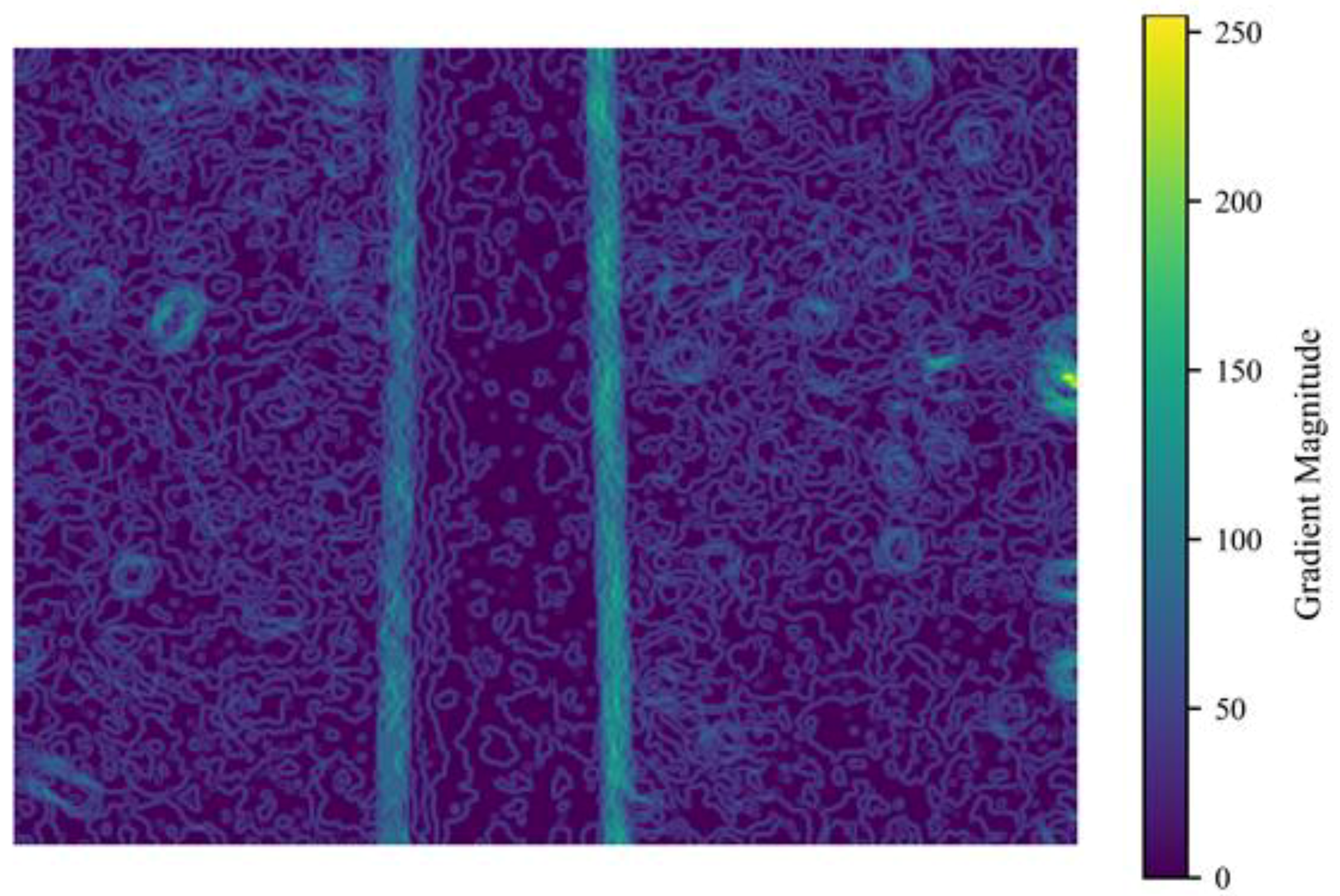
Noise has been effectively reduced while preserving edge information and structural details. Following denoising, the images are processed using Canny edge detection. This widely used edge detection algorithm operates in several steps to identify strong edges based on intensity gradients. The gradient heatmap in Figure 6 highlights the most likely edge points by detecting rapid intensity changes between the riser and the background.

To convert the detected edge pixels into structured line representations, the Hough transform is applied. This classical technique maps points from the image space into a parameter space, typically polar coordinates (ρ, θ), where each edge point votes for all possible lines passing through it. Lines in the image correspond to peaks in this accumulator space, allowing the algorithm to extract the most prominent linear features from noisy or complex edge maps. In this context, the Hough transform helps identify and quantify dominant linear structures from the processed edge image. 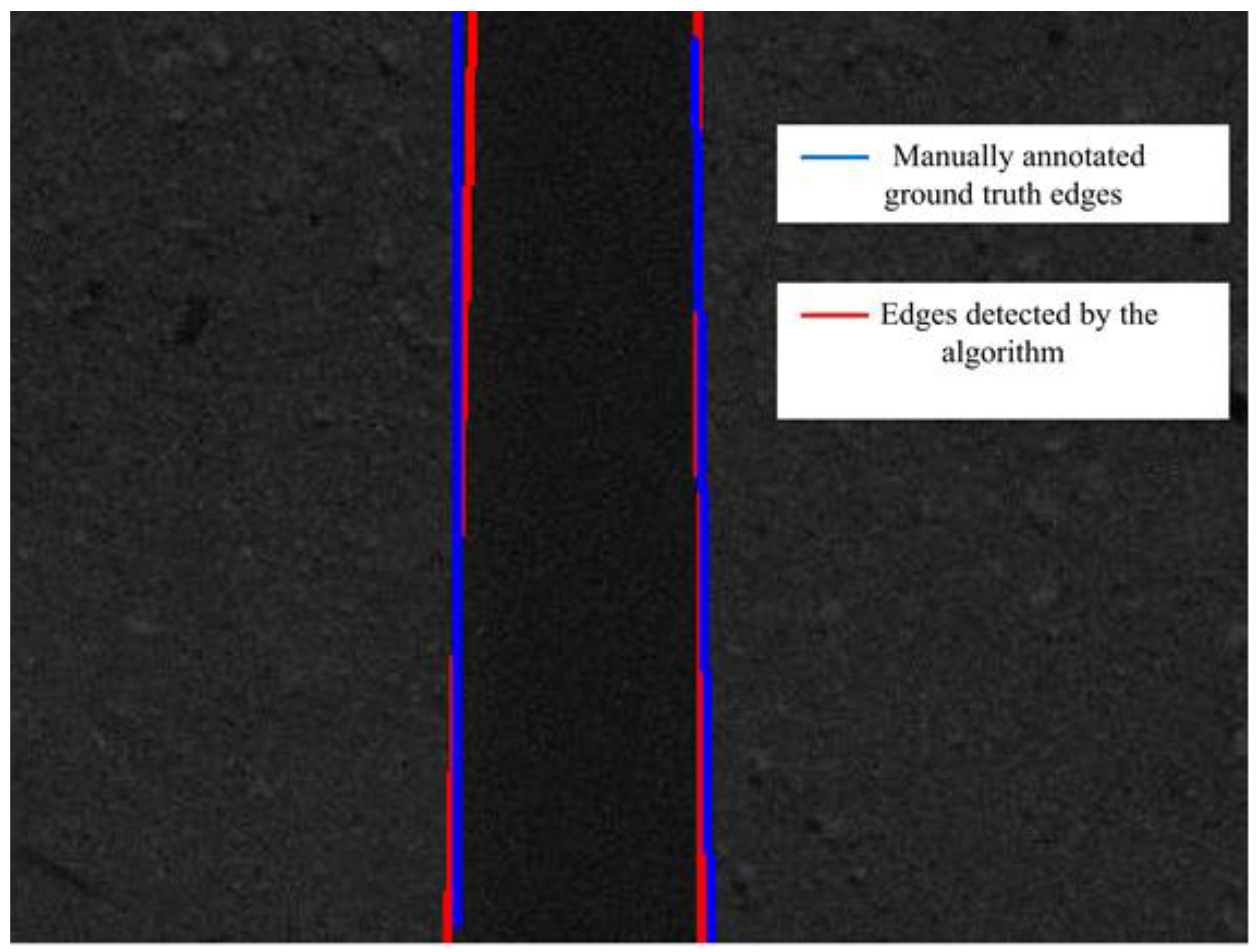Figure 7 presents a visual comparison between the lines detected using the Hough transform (shown in red) and the manually annotated ground truth edges (shown in blue). This overlay provides an intuitive and effective means to assess how well the algorithm captures the actual geometry of the scene and evaluates the precision and consistency of the edge detection process.

The comparison highlights the alignment between algorithmic detection and manually annotated reference edges. Quantitative metrics such as the intersection over union (IoU), Dice Coefficient, F1 score, precision, and recall are summarized in

Table 1. Quantitative metrics evaluating the edge detection algorithm, including precision, recall, F1 score, and accuracy, based on comparison with ground truth edges.

Performance Metric	Value
F1 Score	97.08
Precision	96.68
Recall	97.49
IoU	96.49
Dice Coefficient	98.22

, offering a comprehensive evaluation of the algorithm’s edge detection performance. These metrics are calculated based on pixel-level comparisons between the Hough transform-detected edges and the manually annotated ground truth. As shown in

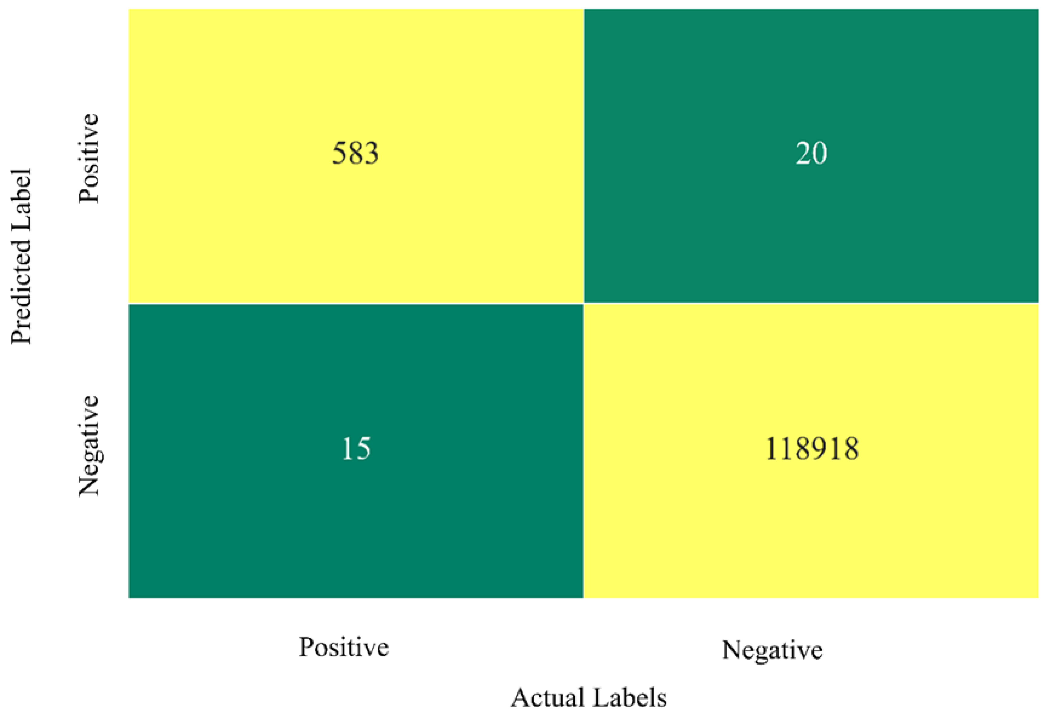
Table 1, the F1 score achieved 97.08%, precision reached 96.68%, recall was 97.49%, IoU was 96.49%, and the Dice Coefficient reached 98.22%. The consistently high values across all metrics indicate that the algorithm accurately detects the riser edges with minimal false positives and false negatives, reflecting strong agreement with the ground truth annotations and confirming the robustness of the edge detection approach. The corresponding confusion matrix is shown in Figure 8, providing a breakdown of classification results. In this matrix, true positives (TP = 583) represent edge pixels that were correctly identified by the algorithm, while true negatives (TN = 118,918) refer to background (non-edge) pixels that were correctly ignored. False positives (FP = 20) indicate background pixels that were incorrectly classified as edges, and false negatives (FN = 15) represent actual edge pixels that the algorithm failed to detect. Together, these values offer both a numerical and visual interpretation of how well the algorithm distinguishes edges from non-edges.

The results demonstrate that, out of approximately 600 strong edge points corresponding to the two riser edges in an image with a height of 300 pixels, the method successfully recognizes the majority of these points. To enhance the realism of the evaluation, a small sliding window is used to count true positive and false positive points. This approach accounts for the narrow pixel width of the edges and ensures precise performance evaluation.

6.2. Detection and Spatial Deviation

To address the challenge posed by irregular and noisy riser edges after the application of the edge detection method described in the previous section, a K-means clustering algorithm was employed. This clustering process was based on the horizontal (x-axis) positions of detected edge pixels. The rationale behind this approach is that true riser edges tend to form two dominant vertical edge clusters, corresponding to the left and right boundaries of the pipe, while noise and false detections are more randomly scattered. By identifying the two clusters with the highest number of members, we effectively filtered out noise and isolated the strongest edge responses derived from the Hough transform output.

The mean positions of these two dominant clusters were then computed and considered as the estimated left and right edges of the riser. The approximate centerline of the riser was calculated as the midpoint between these two means. To evaluate the accuracy of this centerline estimation, the detected center was compared to the known ground truth center in each image frame. The pixel-level deviation between the detected and actual centers was recorded to quantify the localization error across the selected snapshots.

Figure 9 presents the deviation values for each of the 18 snapshots taken along the riser’s geometry path, providing insight into how the algorithm performs across different regions and conditions. Figure 9 illustrates the deviation between the detected center and the true center of the riser, with values ranging from 0 to 23 pixels over the 18 snapshots collected during the tracking process. A deviation of 0 indicates that the method accurately detected the center of the riser, while higher values, such as the 23-pixel deviation observed at snapshot 5, suggest a less precise detection at that point. Overall, most deviations fall within the range of 0–5 pixels, demonstrating strong centerline detection performance, with only a few instances showing deviations between 10 and 23 pixels due to local detection challenges or environmental variations. In addition,

Table 2. Detection metrics—precision, recall, and F1 score—for the 18 sequential snapshots used in the tracking evaluation. These values reflect the algorithm’s performance in accurately identifying the pipe centerline compared to the ground truth in each image.

Snapshot Number	Precision	Recall	F1 Score
1	0.998333333	1	0.999165972
2	0.998310811	0.988294314	0.993277311
3	0.805598756	0.864774624	0.834138486
4	0.704874835	0.897651007	0.789667897
5	0.808868502	0.883138564	0.844373504
6	0.810318665	0.892976589	0.849642005
7	0.840442338	0.889632107	0.864337937
8	0.996621622	0.986622074	0.991596639
9	1	0.92654424	0.96187175
10	0.998236332	0.94490818	0.97084048
11	1	0.936666667	0.967297762
12	0.937799043	0.983277592	0.96
13	1	0.883333333	0.938053097
14	1	0.888333333	0.94086496
15	0.995967742	0.82885906	0.904761905
16	1	0.748333333	0.856053384
17	0.998137803	0.894824708	0.943661972
18	0.998296422	0.978297162	0.988195616

summarizes the detection performance metrics, including precision, recall, and F1 score for the same set of images. These metrics offer a comprehensive evaluation of the method’s ability to distinguish edge pixels from non-edge pixels and reinforce the effectiveness of the proposed detection and center estimation technique. As observed, the highest F1 score of 0.999 was achieved at snapshot 1, indicating near-perfect detection performance. In contrast, lower F1 scores were recorded at snapshots 4 (0.79) and 5 (0.84), suggesting slightly less accurate detection in these regions. This reduction in performance is mainly due to image noise and low contrast between the riser and background in those snapshots. These conditions caused some background pixels to be misclassified as edge points (false positives) and led to missed detections along the riser edges (false negatives), slightly lowering the overall accuracy at those points. Overall, the majority of snapshots maintain high precision and recall values, further demonstrating the robustness and consistency of the algorithm across different sections of the riser.

6.3. Kinematic Analysis of AUV Path Tracking in Simulated Environments

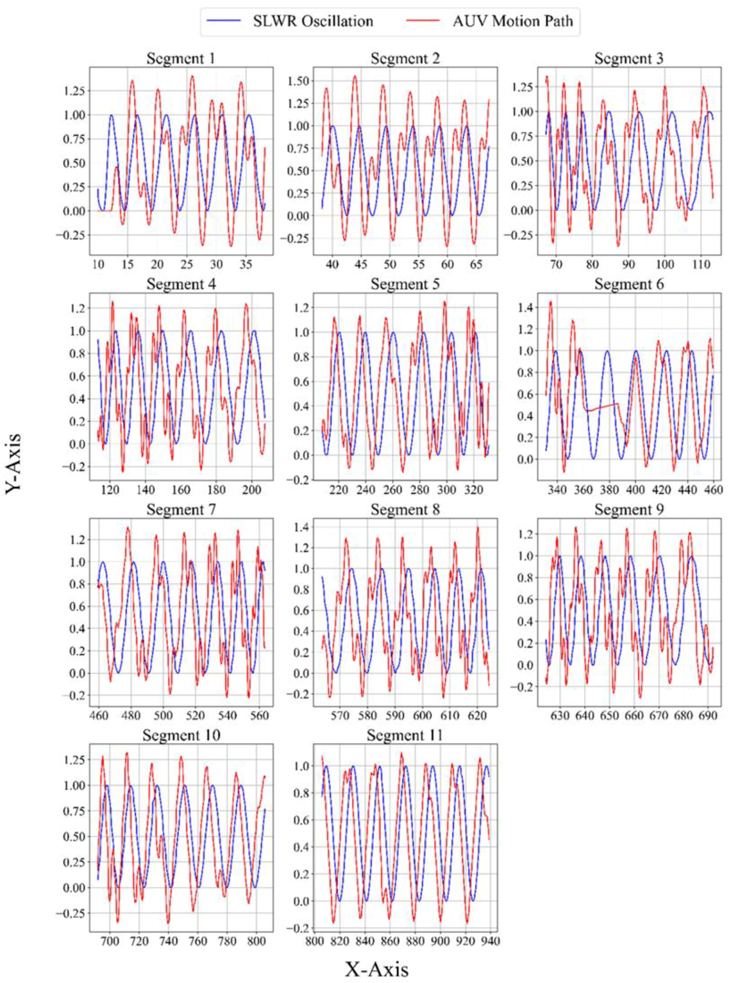
The kinematic analysis of the AUV path tracking was performed within a controlled simulation environment. Figure 10 illustrates the motion trajectory of the AUV in the top view, compared against the oscillatory behavior of the SLWR. For clarity, the path from x = 0 to x = 940 was divided into nine sections for better visualization. In the figure, blue lines represent the oscillations of the riser (y ranging from 0 to 1 meter), while red lines indicate the actual path tracked by the autonomous navigation system. This highlights the AUV’s ability to dynamically update its position based on the riser’s geometry, even when navigating complex regions such as the buoyancy module section. The results demonstrate that the AUV successfully adjusted its lateral position, maintaining alignment with the riser throughout the simulation.

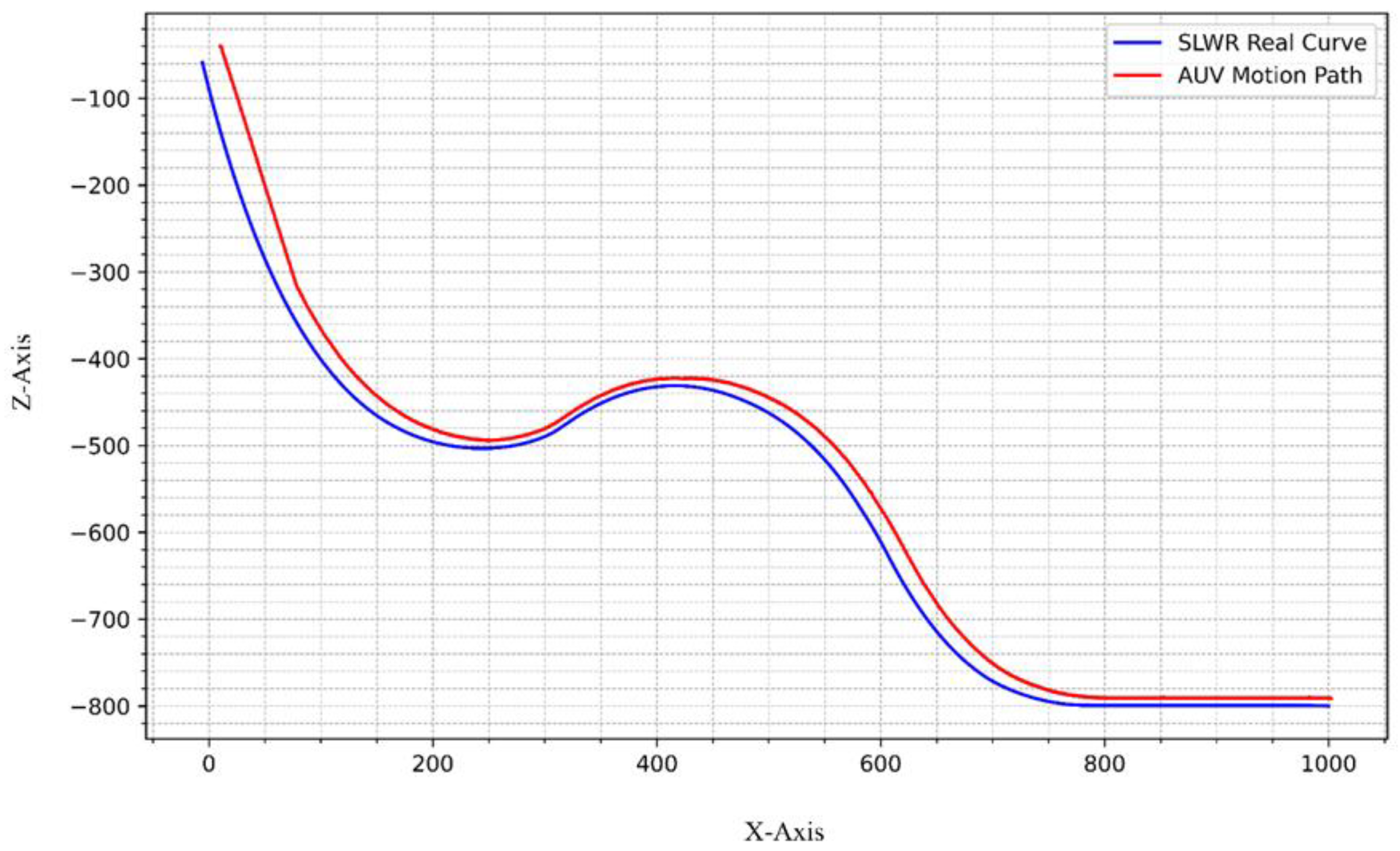
The AUV’s actual path (red) is compared to the SCR position (blue) across divided length segments for clearer analysis. All dimensions are in meters. For a more comprehensive understanding of the AUV’s vertical motion, Figure 11 presents the side view of its trajectory. This perspective emphasizes the AUV’s capability to maintain a specified depth relative to the riser while avoiding collisions in critical regions. Specifically, in the bowl-shaped sections of the SLWR, the AUV effectively adapted its depth to prevent contact with the riser while preserving the required tracking distance. The results confirm that the AUV not only maintained a collision-free path but also accurately followed the riser’s exact curvature, including the challenging sections characterized by oscillations and abrupt depth changes. These findings validate the robustness of the proposed tracking methodology in achieving precise riser-tracking performance under simulated operational conditions.

7. Conclusions

This study successfully demonstrated an AUV equipped with stereo vision and multibeam echosounder sensors for tracking an SLWR while maintaining a safe standoff distance and avoiding structural collisions. The system achieved a high detection F1 score of 92.29%, with an average deviation of only 5.27 pixels from the riser centerline, even under dynamically oscillating conditions in the simulation environment. The AUV effectively followed the riser in both lateral and vertical directions, preserving alignment across spatial planes and maneuvering around buoyancy modules.

Beyond simple detection or inspection, the proposed framework enables precise scanning of the riser’s evolving geometry, particularly in the touchdown zone where seabed–riser interactions gradually alter the structural profile. The spatial data captured through this approach provides a valuable foundation for high-fidelity numerical modeling that incorporates seabed deformation and fatigue behavior. By offering an autonomous solution for generating realistic riser trajectories and cross-sectional profiles, this work contributes to the development of more reliable fatigue life assessments and supports long-term integrity management in offshore infrastructure systems.

It is worth mentioning that the current study has been conducted in a simulation environment that can be a simplified version of the real environment. In the future phases of the project, the algorithms shall be uploaded to the onboard computer of a real AUV and the efficiency of the algorithms in terms of time and memory size in a real environment are required to be assessed by performing a computational complexity analysis to ensure there will be no delay in the control system. This cannot be conducted in a simulated environment because of the scaling challenges and the limitations in simultaneous simulation of the first- and second-order AUV motions along with riser’s hydrodynamic response to the sea currents in the software. These field tests are mandatory to assess the practicality of the proposed algorithms.