Trajectory Tracking of Unmanned Surface Vessels Based on Robust Neural Networks and Adaptive Control

Abstract

In this paper, a robust neural adaptive controller is proposed for the trajectory tracking control problem of unmanned surface vessels (USVs), considering model uncertainty, time-varying environmental disturbance, and actuator saturation. First, measurement errors in acceleration signals are eliminated through filtering techniques and a series of auxiliary variables, and after linearly parameterizing the USV dynamic model, a parameter adaptive update law is developed based on Lyapunov’s second method to estimate unknown dynamic parameters in the USV dynamics model. This parameter adaptive update law enables online identification of all USV dynamic parameters during trajectory tracking while ensuring convergence of the estimation errors. Second, a radial basis function neural network (RBF-NN) is employed to approximate unmodeled dynamics in the USV system, and on this basis, a robust damping term is designed based on neural damping technology to compensate for environmental disturbances and unmodeled dynamics. Subsequently, a trajectory tracking controller with parameter adaptation law and robust damping term is proposed using Lyapunov theory and adaptive control techniques. In addition, finite-time auxiliary variables are also added to the controller to handle the actuator saturation problem. Signal delay compensators are designed to compensate for input signal delays in the control system, thereby enhancing controller reliability. The proposed controller ensures robustness in trajectory tracking under model uncertainties and time-varying environmental disturbances. Finally, the convergence of each signal of the closed-loop system is proved based on Lyapunov theory. And the effectiveness of the control system is verified by numerical simulation experiments.

1. Introduction

With the increasing scarcity of land resources, the development of marine resources by humans is an important trend in future development. Unmanned surface vehicles (USVs) are water robots that can navigate unmanned, autonomously, and highly maneuverably on the water surface and are often used to perform specific tasks such as maritime patrol, meteorological monitoring, anti-submarine and mine clearance in complex waters; therefore, USVs have important research value and broad research prospects in both military and civilian fields [1]. As an important technical link of USV autonomous navigation, the motion control of USVs can be divided into positioning control [2,3,4], path following [5,6,7], and trajectory tracking [8,9,10] according to different control objectives. Among them, the trajectory tracking of USVs specifically refers to the design of the controller of the USV so that the USV can not only navigate according to the preset route, but also reach the specified position on the route at the specified time. It can be seen that the accurate tracking of the desired trajectory by USV is of great significance for improving the autonomous navigation of USVs.

In the dynamic model of USVs, the precision of the dynamic parameters that reflect the inertial characteristics and hydrodynamic characteristics of the USV is particularly crucial for achieving accurate trajectory tracking of the USV. The dynamic parameters of USVs with different ship types vary. These USV dynamic parameters usually need to be obtained through costly ship maneuverability experiments. However, these dynamic parameters are unknown in many application scenarios. Due to the complex interaction mechanism between USVs and water, the dynamic models of USVs established by researchers from various countries at present are difficult to accurately describe the motion of the USV. Therefore, there are unmodeled parts in the dynamic models that are currently used to describe the motion of the USV. This, together with the uncertainty of the USV dynamic parameters, results in the uncertainty of the USV model. At the same time, the USV will be subjected to unknown time-varying environmental disturbances during the navigation process. The model uncertainty and the unknown time-varying environmental disturbances pose great challenges to achieving the trajectory tracking of the USV.

Benefiting from the development of nonlinear control theory, neural networks, and other technologies, in recent years, scholars from various countries have conducted some studies of USV trajectory tracking using the backstep method, model predictive control, robust control, reinforcement learning, and other methods. Wang designed a trajectory tracking controller for underactuated USVs based on backstepping control method and fuzzy neural networks and designed event triggering conditions for updating the controller according to Lyapunov function [11]. Yuan simplified the USV dynamic model into a discrete form and designed the controller by combining model predictive control (MPC) and the event-triggered mechanism to track the trajectory during the autonomous berthing process of the USV [12]. Sami designed a sliding mode controller with a time-varying boundary layer to solve the problem of trajectory tracking of USVs with unknown environmental disturbances [13]. Zheng designed a nonlinear active disturbance rejection controller to achieve trajectory tracking of USVs, and improved the performance of the controller by adapting the design parameters of the controller through the reinforcement learning DDPG algorithm [14]. The above studies all have high requirements for the accuracy of prior information on dynamic parameters.

As an important nonlinear control method, adaptive control technology automatically adjusts the unknown parameters in the controller through the feedback signals of the dynamic system, which has certain advantages in solving the motion control problem of the USV when the dynamic parameters are unknown. For the heading control problem of USVs under disturbances, Liu proposed a novel data-driven adaptive sliding mode controller based on Model-Free Adaptive Control (MFAC) theory [15]. Souissi designed an adaptive law with alternative leakage terms based on composite adaptive technology to compensate for the impact of the uncertainty of USV dynamic parameters on USVs, and thus designed a trajectory tracking controller for USVs [16]. Xiong proposed a data-driven interactive identification algorithm based on an extended state observer (ESO) to online identify USV dynamic parameters and estimate environmental disturbances, achieving adaptive motion control [17]. Wang developed an improved data-driven disturbance observer for environmental disturbance estimation and proposed a model-free adaptive controller for USVs [18]. Neural networks can be used to approximate uncertain models and have been applied to some extent in the research of USV motion control [19,20,21]. Under the framework of adaptive control technology, combining adaptive control with technologies such as neural networks brings the possibility of achieving the trajectory tracking of USVs under model uncertainty and environmental disturbances. Zhang proposed an adaptive trajectory tracking controller with a high-gain observer that compensates for the model uncertainty through the RBF-NNs and a second-order differentiator [22]. Meng used a Bidirectional Long Short-Term Memory (BiLSTM) neural network to approximate the uncertain model of the USV, and thus proposed a robust adaptive trajectory tracking controller for USV [23]. However, the above-mentioned studies failed to consider the unmodeled parts in the dynamic model of the USV, and it is difficult to identify the actual values of the uncertain dynamic parameters.

To enhance the robustness of USVs in trajectory tracking under model uncertainties and environmental disturbances, this paper proposes a robust neural adaptive controller by separately addressing the unknown dynamic parameters and the unmodeled dynamics in the uncertain model. Firstly, a series of filters and auxiliary variables are designed to eliminate measurement errors in acceleration signals. After linearly parameterizing the USV dynamic model, an adaptive update law for the unknown dynamic parameters is developed. The Radial Basis Function Neural Networks (RBF-NNs) are employed to approximate the unmodeled dynamics in the USV dynamic model. Additionally, auxiliary variables are designed to handle actuator saturation. Subsequently, a controller with a dynamic parameters adaptive update law is designed based on robust neural damping techniques to achieve trajectory tracking for the USV. Then, the convergence of all signals in the closed-loop system is proven using Lyapunov theory. Finally, the effectiveness of the proposed method is validated through simulation experiments. The main contributions of this paper are summarized as follows:

(1)

A robust neural adaptive trajectory tracking controller is designed to achieve trajectory tracking for USVs under conditions when the dynamic parameters are unknown, have unmodeled dynamics in the dynamic model, have unknown time-varying environmental disturbances, and have actuator saturation constraints.

(2)

The controller separately addresses the unknown dynamic parameters and the unmodeled dynamics in the uncertain model. In the controller, the RBF-NNs are employed to approximate the unmodeled dynamics, while robust neural damping techniques are used to compensate for the unknown time-varying environmental disturbances and the unmodeled dynamics.

(3)

The controller incorporates a parameter adaptive update law for online identification of all USV dynamic parameters. This ensures convergence of both parameter estimation errors and tracking errors when dynamic parameters are unknown or perturbed.

The remainder of this paper is organized as follows. Section 2 establishes the three-degree-of-freedom (3-DOF) USV model and defines the trajectory tracking problem for the USV. Section 3 details the design of the controller and provides the proof of convergence for all signals in the closed-loop system. Section 4 analyzes the process and results of the simulation experiments. Section 5 concludes the paper.

2. Problem Formulation

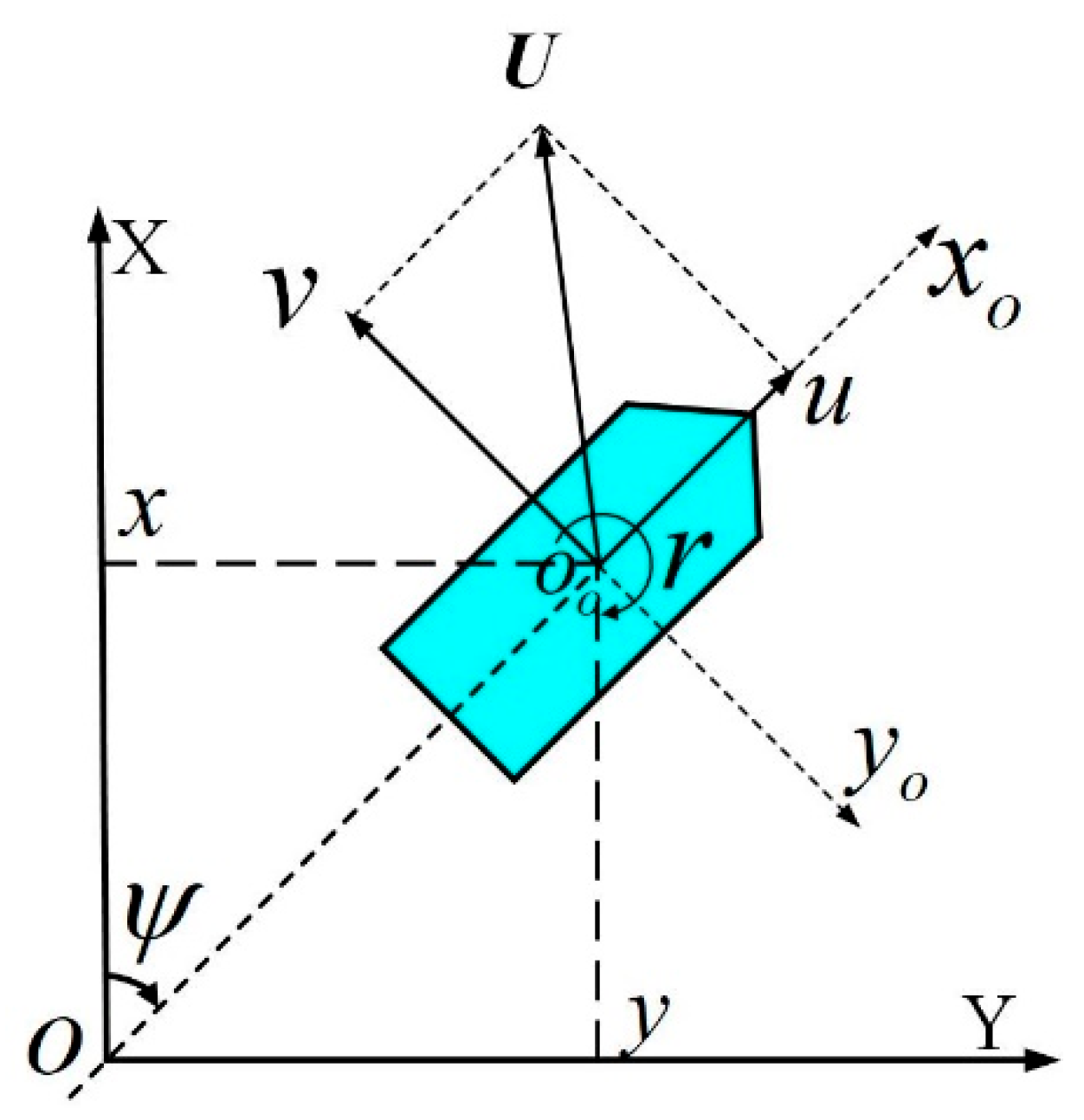
Throughout the paper, $\left|\ast \right|$ denotes the absolute value of a scalar, $‖\ast ‖$ represents the Euclidean norm of a vector, and ${‖\ast ‖}_F$ denotes the Frobenius norm of a vector. $\widehat{\left(\ast \right)}$ denotes the estimate of $\left(\ast \right)$, and $\widetilde{\left(\ast \right)}=\widehat{\left(\ast \right)}-\left(\ast \right)$ represents the estimation error. $\overline{\left(\ast \right)}$ indicates the upper bound of a variable. This section designs the 3-degree-of-freedom (3-DOF) USV model, provides an explanation of actuator saturation, and describes the trajectory tracking problem.

2.1. USV Model

To facilitate the description of the three-degree-of-freedom (3-DOF) motion of the USV on the horizontal plane, a space-fixed coordinate system $O-XYZ$ is established, as shown in Figure 1. In this system, the $OX$ axis points to the north, and the $OY$ axis points to the east. The coordinates $(x,y)$ represent the position of the USV’s midship in the $O-XYZ$ coordinate system, and $\psi$ denotes the heading angle of the USV. Simultaneously, a body-fixed coordinate system $O_{\mathrm{o}}-x_{\mathrm{o}}{y}_{\mathrm{o}}{z}_{\mathrm{o}}$ is established with the USV’s midship $O_{\mathrm{o}}$ as the origin. In this system, $u$, $v$, and $r$ represent the surge velocity, sway velocity, and yaw rate of the USV, respectively. The kinematic model of the USV describes the relationship between the USV’s velocity and its position coordinates. The kinematic model of the USV is given by Equation (1):

$$\dot{\eta }=R\left(\psi \right)\mathbf{v}$$

(1)

In Equation (1), ${\eta }^T=[x,y,\psi ]$, ${\mu }^T=[u,v,r]$, and $R\left(\psi \right)$ is the bow roll rotation matrix, defined as:

$$R\left(\psi \right)=\left[\begin{array}{ccc}cos\psi & -sin\psi & 0\\ sin\psi & cos\psi & 0\\ 0& 0& 1\end{array}\right]$$

(2)

The dynamic model of the USV is used to describe the relationship between the forces acting on the USV and its velocity and acceleration. With reference to [24,25], the dynamic model of the USV is expressed by Equation (3):

$$M\dot{\mathbf{v}}+C\left(\mathbf{v}\right)\mathbf{v}+D\left(\mathbf{v}\right)\mathbf{v}=\tau +f$$

(3)

In Equation (3), ${\tau }^T={[\tau }_1,$ ${\tau }_2,$ ${\tau }_3$] represents the control forces of the USV in the three degrees of freedom on the horizontal plane, which also serve as the control input vector for the USV’s trajectory tracking. $f^T={[f}_1,$ $f_2,$ $f_3$] denotes the environmental disturbance force vector. $M=M_0+∆M$ is the inertia matrix, $D\left(\mathbf{v}\right)=D_0\left(\mathbf{v}\right)+∆D\left(\mathbf{v}\right)$ is the damping matrix, and $C\left(\mathbf{v}\right)=C_0\left(\mathbf{v}\right)+∆C\left(\mathbf{v}\right)$ is the Coriolis and centripetal force matrix. Here, $M_0$ is a symmetric positive definite matrix, and ${\mathrm{M}}_0$, ${\mathrm{D}}_0\left(\mathbf{v}\right)$, and ${\mathrm{C}}_0\left(\mathbf{v}\right)$ represent the nominal parts of $\mathrm{M}$, $\mathrm{D}\left(\mathbf{v}\right)$, and $\mathrm{C}\left(\mathbf{v}\right)$, respectively. $∆\mathrm{M}$, $∆\mathrm{D}\left(\mathbf{v}\right)$, and $∆\mathrm{C}\left(\mathbf{v}\right)$ denote the unmodeled parts of $\mathrm{M}$, $\mathrm{D}\left(\mathbf{v}\right)$, and $\mathrm{C}\left(\mathbf{v}\right)$, respectively. The specific forms of ${\mathrm{M}}_0$, ${\mathrm{D}}_0\left(\mathbf{v}\right)$, and ${\mathrm{C}}_0\left(\mathbf{v}\right)$ are as follows:

$$M_0=\left[\begin{array}{ccc}{m}_{11}& 0& 0\\ 0& m_{22}& m_{23}\\ 0& m_{32}& m_{33}\end{array}\right]$$

(4)

$$\begin{array}{c}{D}_0\left(\mathbf{v}\right)\\ =\left[\begin{array}{ccc}-X_u-X_{u\left|u\right|}\left|u\right|& 0& 0\\ 0& {-Y}_v-Y_{v\left|v\right|}\left|v\right|-Y_{\left|r\right|v}\left|r\right|& {-Y}_r-Y_{\left|v\right|r}\left|v\right|-Y_{r\left|r\right|}\left|r\right|\\ 0& -N_v-N_{v\left|v\right|}\left|v\right|-N_{\left|r\right|v}\left|r\right|& -N_r-N_{\left|v\right|r}\left|v\right|-N_{r\left|r\right|}\left|r\right|\end{array}\right]\end{array}$$

(5)

$$C_0\left(\mathbf{v}\right)=\left[\begin{array}{ccc}0& 0& -m_{22}v-m_{23}r\\ 0& 0& m_{11}u\\ m_{22}v+m_{23}r& -m_{11}u& 0\end{array}\right]$$

(6)

In Equations (4)–(6), $m_{11}=m-X_{\dot{u}}$, $m_{22}=m-Y_{\dot{v}}$, $m_{23}=m_{32}=m{x}_g-Y_{\dot{r}}$, $m_{33}=I_Z-N_{\dot{r}}$. Among them, $m$ is the mass of the USV, and $x_g$ is the coordinate of the center of gravity of the USV in the body-fixed coordinate system, $X_{\dot{u}}$, $Y_{\dot{v}}$, $Y_{\dot{r}}$, and $N_{\dot{r}}$ are coefficients that reflect the additional mass of the USV. $X_u,X_{u\left|u\right|},Y_v,Y_r,Y_{v\left|v\right|},Y_{\left|r\right|v},Y_{\left|v\right|r},Y_{r\left|r\right|},N_v,N_r,N_{v\left|v\right|},N_{\left|r\right|v},N_{\left|v\right|r}$, and $N_{r\left|r\right|}$ all are hydrodynamic coefficients.

2.2. Actuator Saturation

The control forces of the USV are typically generated by actuators such as rudders and propellers. Depending on the specific mission of the USV, different actuators may be installed. For the trajectory tracking of the USV, it is usually only necessary to determine the control forces that need to be applied to the USV. After obtaining these control forces, specific actuator commands, such as propeller speed or rudder angle, can be obtained through thrust allocation algorithms based on the actual actuator configuration of the USV [26]. Due to factors such as material limitations, dimensional parameters, and mechanical friction, the control forces generated by the USV actuators are subject to saturation constraints as shown in Equation (7):

$${\tau }_i=\left\{\begin{array}{ll}{\tau }_{Mi}& {\tau }_{0i}\ge {\tau }_{Mi}\\ {\tau }_{0i}& {-\tau }_{Mi}<{\tau }_{0i}<{\tau }_{Mi}\\ {-\tau }_{Mi}& {\tau }_{0i}\le {-\tau }_{Mi}\end{array}\right.$$

(7)

In the above equation, ${\tau }_{Mi}$ represents the maximum control force that the USV actuator can generate in the $i$-th degree of freedom, and ${\tau }_{0i}$ denotes the output of the controller in the $i$-th degree of freedom. Let $∆\tau =\tau -{\tau }_0$ be the deviation between the controller output and the actual control force.

2.3. Definition of USV Trajectory Tracking

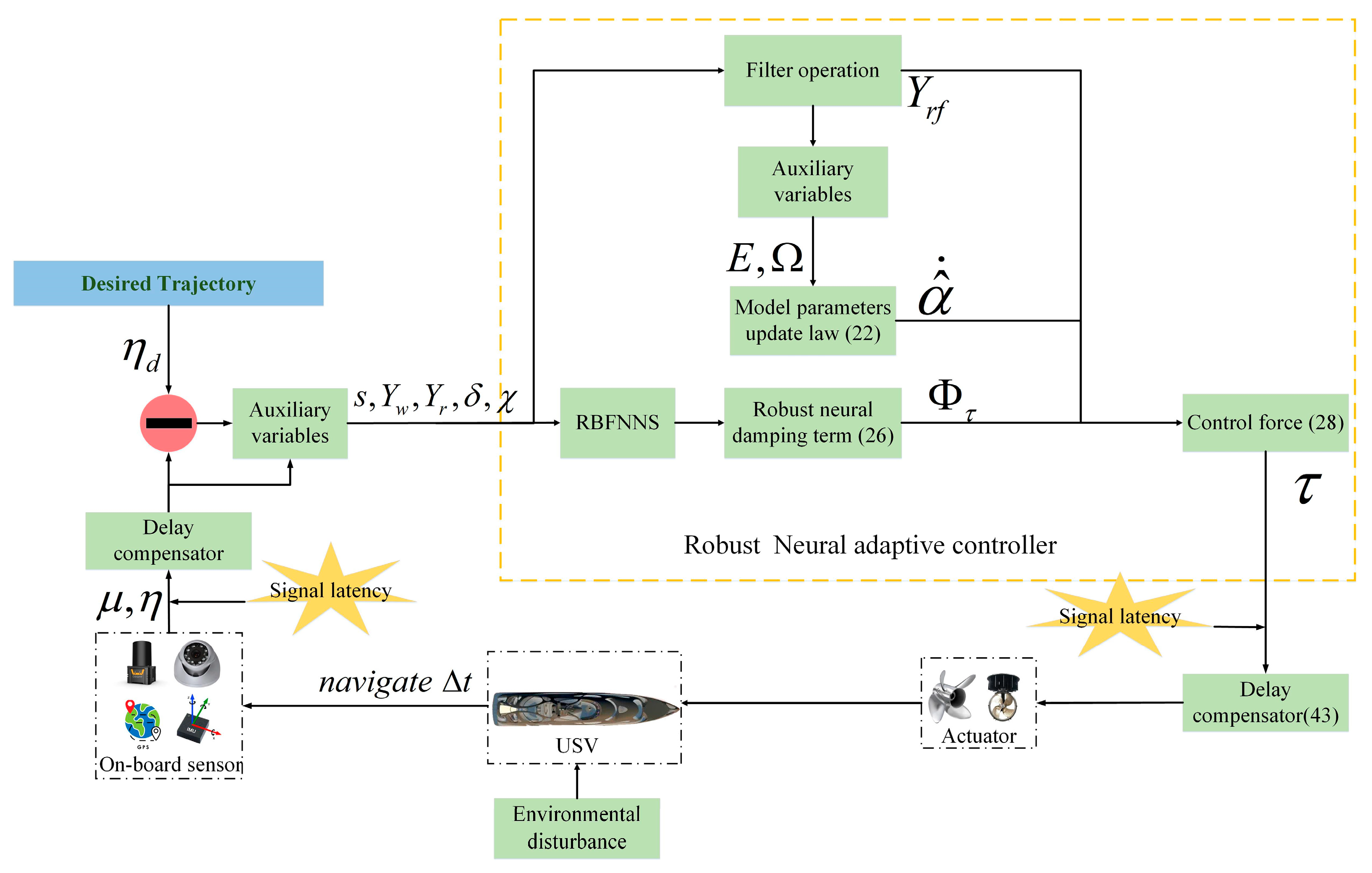
Define the desired trajectory ${\eta }_d^T=[x_d,y_d,{\psi }_d]$ and the desired velocity ${\mathbf{v}}_d^T=[u_d,v_d,r_d]$ for the USV trajectory tracking. Define the tracking errors for the desired trajectory and the desired velocity as $\tilde{\eta }=\eta -{\eta }_d={[\tilde{x},\tilde{y},\tilde{\psi }]}^T$ and $\tilde{\mathbf{v}}=\mathbf{v}-{\mathbf{v}}_d={[\tilde{u},\tilde{v},\tilde{r}]}^T$, respectively. Based on the USV dynamic model shown in Equation (3), let the dynamic parameters vector $\alpha \in R^p$ denote all parameters in the USV dynamic model. The specific form of $\alpha$ is as follows:

$${\alpha }^T=[X_u,Y_v,Y_r,N_v,N_r,X_{u\left|u\right|},Y_{v\left|v\right|},Y_{\left|v\right|r},Y_{\left|r\right|v},Y_{r\left|r\right|},N_{v\left|v\right|},N_{\left|v\right|r},N_{\left|r\right|v},N_{r\left|r\right|},m_{11},m_{22},m_{23},m_{33}]$$

Equation (3) can be further expanded as follows:

$$M_0\dot{\mathbf{v}}+C_0\left(\mathbf{v}\right)\mathbf{v}+D_0\left(\mathbf{v}\right)\mathbf{v}+∆M\dot{\mathbf{v}}+∆C\left(\mathbf{v}\right)\mathbf{v}+∆D\left(\mathbf{v}\right)\mathbf{v}=\tau +f$$

(8)

Let $f_d=∆M\dot{\mathbf{v}}+∆C\left(\mathbf{v}\right)\mathbf{v}+∆D\left(\mathbf{v}\right)\mathbf{v}$ represent the unmodeled dynamics. To accurately describe the USV trajectory tracking problem addressed in this paper, the following assumptions are made:

Assumption 1.

The desired trajectory ${\eta }_d^T=[x_d,y_d,{\psi }_d]$ is smooth and bounded, and the first and second derivatives of the desired trajectory ${\eta }_d$ are also bounded. There exist normal numbers ${\rho }_i,i=\mathrm{1,2},3$ and ${\sigma }_i,i=\mathrm{1,2}$ , such that $‖{\eta }_d‖\le {\rho }_1$, $‖\dot{{\eta }_d}‖\le {\rho }_2$, $‖\ddot{{\eta }_d}‖\le {\rho }_3$.

Assumption 2.

All dynamic parameters in the dynamic parameters vector $\alpha$ are unknown.

Assumption 3.

The unmodeled dynamics $f_d$ are unknown and bounded.

Assumption 4.

The time-varying environmental disturbances $f$ acting on the USV are unknown and have an upper bound $\overline{f}$.

According to Assumption 2, let $\widehat{\alpha }$ denote the estimate of the dynamic parameters $\alpha$. The estimation error of the dynamic parameters is defined as $\tilde{\alpha }=\widehat{\alpha }-\alpha$.

Control Problem: For the USV which kinematics and dynamics can be characterized by Equations (1)–(7) and satisfies Assumptions 1–4, the control objective of trajectory tracking is to design the control input $\tau$ and the adaptive update law for the dynamic parameters $\alpha$ such that all signals in the closed-loop system, including $\tilde{\eta }$, $\tilde{\mathbf{v}}$, and $\tilde{\alpha }$, are semi-globally uniformly ultimately bounded (SGUUB), when the desired trajectory satisfies Assumption 1.

Remark 1.

As a weak stability theory, SGUUB enables the USV to maintain robustness against external disturbances and model uncertainties, ensuring that the USV’s states (e.g., position, velocity, heading) are ultimately confined within predetermined bounds. Even in the presence of external disturbances (e.g., wind waves, sensor noise), the trajectory of the USV will not exceed safe limits or deviate from the operational area. This guarantees that USVs performing long-term missions (e.g., environmental monitoring, cargo transportation) remain within acceptable operational ranges. Therefore, the proposed controller ensures that the trajectory tracking error of the USV is SGUUB, which is both effective and reasonable for practical engineering applications.

3. Controller

This section begins with the linear parameterization of the USV dynamic model, followed by the design of a set of auxiliary variables incorporating the error signals of the closed-loop system. Based on this, an adaptive update law for the dynamic parameters is formulated. Subsequently, robust neural damping techniques are introduced to compensate for environmental disturbances and model uncertainties. Auxiliary variables are designed to handle the problem of input saturation of actuators. And on the basis of the above design, the control law is designed. Finally, the convergence of all signals in the closed-loop system is proved based on Lyapunov theory. The calculation block diagram of the proposed controller is illustrated in Figure 2.

3.1. Controller Design

3.1.1. Step 1: Design of Auxiliary Variables Incorporating Error Signals

An error variable as shown in Equation (9) is defined to measure the trajectory tracking error of the USV.

$$s=\dot{\tilde{\eta }}+\mathsf{\Lambda }\tilde{\eta }+{\xi }_s$$

(9)

In the above equation, $s^T=\left[s_1,s_2,s_3\right]$. ${\xi }_s>0$ is a small numerical parameter that ensures the non-singularity of $‖s‖$ during the initial period, thereby preventing computational errors in the control system. Additionally, $\mathsf{\Lambda }=diag\left({\lambda }_1,{\lambda }_2,{\lambda }_3\right)$, and ${\lambda }_i>0$. The term $M_0\dot{\mathbf{v}}+C_0\left(\mathbf{v}\right)\mathbf{v}+D_0\left(\mathbf{v}\right)\mathbf{v}$ in Equation (8) can be linearly parameterized as follows:

$$M_0\dot{\mathbf{v}}+C_0\left(\mathbf{v}\right)\mathbf{v}+D_0\left(\mathbf{v}\right)\mathbf{v}=Y_w\alpha$$

(10)

In the above equation, $Y_w\in R^{3\times p}$. After substituting Equations (4)–(6) into Equation (10), we obtain the specific form of $Y_w$ as follows:

$$\left[\begin{array}{cccccccccccccccccc}-u& 0& 0& 0& 0& -\left|u\right|u& 0& 0& 0& 0& 0& 0& 0& 0& \dot{u}& -vr& -r^2& 0\\ 0& -v& -r& 0& 0& 0& -\left|v\right|v& -\left|v\right|r& -\left|r\right|v& -\left|r\right|r& 0& 0& 0& 0& ur& \dot{v}& \dot{r}& 0\\ 0& 0& 0& -v& -r& 0& 0& 0& 0& 0& -\left|v\right|v& -\left|v\right|r& -\left|r\right|v& -\left|r\right|r& -uv& uv& \dot{v}+ur& \dot{r}\end{array}\right]$$

In order to eliminate the high-frequency noise in the USV acceleration signal and facilitate the design of the adaptive update law of the dynamic parameters. We define the auxiliary variables $\mathsf{\Omega }\in R^{p\times p}$, $\Gamma \in R^{p\times 1}$, and $F\in R^{p\times 1}$ as follows:

$$\dot{\mathsf{\Omega }}=-\mathsf{\Omega }+Y_w^T{Y}_w+{\xi }_{\alpha }$$

(11)

$$\dot{\Gamma }=-\Gamma +Y_w^T\tau$$

(12)

$$\dot{F}=-F+Y_w^T(f-f_d)$$

(13)

In Equation (11), ${\xi }_{\alpha }>0$ is a small numerical parameter that ensures the non-singularity of $‖\mathsf{\Omega }‖$ during the initial period. Equations (11)–(13) can be regarded as first-order low-pass filters applied to the input signals $Y_w^T{Y}_w+{\xi }_{\alpha }$, $Y_w^T\tau$, and $Y_w^T(f-f_d)$, thereby eliminating high-frequency noise of these input signals. $Y_w\tilde{\alpha }=Y_w\widehat{\alpha }-\alpha =Y_w\widehat{\alpha }-\tau -(f-f_d)$; therefore, according to Equation (12), it can be seen that $\Gamma =\mathsf{\Omega }\alpha -F$. Define auxiliary variables that contain the dynamic parameters information as follows:

$$E=\mathsf{\Omega }\widehat{\alpha }-\Gamma =\mathsf{\Omega }\tilde{\alpha }+F$$

(14)

From the above equation, it can be observed that ${\mathsf{\Omega }}^{-1}E=\tilde{\alpha }+\omega$, where $\omega ={\mathsf{\Omega }}^{-1}F={\mathsf{\Omega }}^{-1}\left(\mathsf{\Omega }\alpha -\Gamma \right)=\alpha -{\mathsf{\Omega }}^{-1}\Gamma$. According to Assumption 3 and Assumption 4, both $f$ and $f_d$ are bounded. Consequently, $\omega$ and $\dot{\omega }$ can be considered bounded. That is, there exist positive constants ${\varrho }_1$ and ${\varrho }_2$ such that: $‖\omega ‖\le {\varrho }_1$, $‖\dot{\omega }‖\le {\varrho }_2$.

Remark 2.

It can be seen from Equation (11) that: $\Omega ={\int }_0^t{e}^{-\mathcal{l}(t-r)}\left(Y_w^T\left(r\right)Y_w\left(r\right)+{\xi }_{\alpha }\right)dr={\int }_{t-dt}^t{e}^{-\mathcal{l}dt}{Y}_w^T\left(r\right)Y_w\left(r\right)dr+{\int }_{t-dt}^t{e}^{-\mathcal{l}dt}{\xi }_{\alpha }dr$. Due to $Y_w^T\left(r\right)Y_w\left(r\right)\ge 0$, ${\xi }_{\alpha }>0$. Thus, ${\int }_{t-dt}^t{e}^{-\mathcal{l}dt}{Y}_w^T\left(r\right)Y_w\left(r\right)dr\ge 0$, ${\int }_{t-dt}^t{e}^{-\mathcal{l}dt}{\xi }_{\alpha }dr>e^{-\mathcal{l}T}{\xi }_{\alpha }$. Therefore, when there exists $dt>0, \Omega >e^{-\mathcal{l}T}{\xi }_{\alpha }>0$ is true for all $t>0$ and $\sigma =e^{-\mathcal{l}T}{\xi }_{\alpha }$. Consequently, $\Omega$ is positive definite $({\lambda }_{min}\left(\Omega \right)>\sigma >0)$.

3.1.2. Step 2: Design of Dynamic Parameters Adaptive Update Law

A positive definite candidate Lyapunov function is defined as follows:

$$V={\displaystyle \frac{1}{2}}{s}^T{M}_{0}s+{\displaystyle \frac{1}{2}}{E}^T{\mathsf{\Omega }}^{-1}{P}^{-1}{\mathsf{\Omega }}^{-1}E$$

(15)

In the above equation, $P^{-1}=pI$, $p$ positive design parameters. Taking the time derivative of Equation (15), we obtain:

$$\dot{V}=s^T{M}_0\dot{s}+{(\dot{\tilde{\alpha }}+\dot{\omega })}^T{P}^{-1}{\mathsf{\Omega }}^{-1}E$$

(16)

To facilitate the design of the controller, an auxiliary variable ${\mu }_s$ is defined as follows:

$${\mathbf{v}}_s=\mathbf{v}-s$$

(17)

In the above equation, ${\mathbf{v}}_s^T=[{\mathbf{v}}_{s1},{\mathbf{v}}_{s2},{\mathbf{v}}_{s3}]$. During a single voyage, the loading condition of the USV typically remains unchanged, and the mass reduction due to energy consumption can be neglected. Additionally, the hydrodynamic coefficients of the USV, which are primarily determined by the hull shape, usually exhibit minimal variation during navigation. Therefore, the model parameters $\alpha$ can be considered constant or slowly time-varying, i.e., $\dot{\tilde{\alpha }}=\dot{\widehat{\alpha }}$. Substituting Equations (8) and (17) into Equation (16), we obtain:

$$\dot{V}=s^T\left(M_0\dot{\mathbf{v}}-M_0{\dot{\mathbf{v}}}_{\mathit{s}}\right)+{(\dot{\widehat{\alpha }}+\dot{\omega })}^{T}P{\mathsf{\Omega }}^{-1}=s^T\left(\tau +f-f_d-C_0\left(\mathbf{v}\right)\mathbf{v}-D_0\left(\mathbf{v}\right)\mathbf{v}-M_0{\dot{\mathbf{v}}}_{\mathit{s}}\right)+{\dot{\widehat{\alpha }}}^{T}P{\mathsf{\Omega }}^{-1}E+{\dot{\omega }}^{T}P{\mathsf{\Omega }}^{-1}E$$

(18)

In Equation (18), $C_0\left(\mathbf{v}\right)\mathbf{v}+D_0\left(\mathbf{v}\right)\mathbf{v}+M_0{\dot{\mathbf{v}}}_s$ can be linearly parameterized as follows:

$$C_0\left(\mathbf{v}\right)\mathbf{v}+D_0\left(\mathbf{v}\right)\mathbf{v}+M_0{\dot{\mathbf{v}}}_s=Y_r\alpha$$

(19)

Among them, $Y_r\in R^{3\times p}$, the specific form of $Y_r$ as follows:

$$\left[\begin{array}{cccccccccccccccccc}-u& 0& 0& 0& 0& -\left|u\right|u& 0& 0& 0& 0& 0& 0& 0& 0& {\dot{\mathbf{v}}}_{s1}& -vr& -r^2& 0\\ 0& -v& -r& 0& 0& 0& -\left|v\right|v& -\left|v\right|r& -\left|r\right|v& -\left|r\right|r& 0& 0& 0& 0& ur& {\dot{\mathbf{v}}}_{s2}& {\dot{\mathbf{v}}}_{s3}& 0\\ 0& 0& 0& -v& -r& 0& 0& 0& 0& 0& -\left|v\right|v& -\left|v\right|r& -\left|r\right|v& -\left|r\right|r& -uv& uv& {\dot{\mathbf{v}}}_{s2}+ur& {\dot{\mathbf{v}}}_{s3}\end{array}\right]$$

To eliminate the high-frequency noise of the acceleration signal in $Y_r$, put $Y_r$ into the first-order low-pass filter as follows:

$${{k_r\dot{Y}}_{rf}+Y}_{rf}=Y_r$$

(20)

In the above equation, $k_r>0$ is a design parameter, and $Y_{rf}$ represents the filtered output signal of $Y_r$. Let $d_1=Y_r-Y_{rf}$ denote the filtering error between $Y_r$ and $Y_{rf}$, such that $Y_r\alpha =\left(d_1+Y_{rf}\right)\alpha =d_1\alpha +Y_{rf}\alpha$. Substituting Equation (19) into Equation (18), we obtain:

$$\dot{V}=s^T\left(\tau +f-f_d-d_1\alpha -Y_{rf}\alpha \right)+{\dot{\widehat{\alpha }}}^T{P}^{-1}{\mathsf{\Omega }}^{-1}E+{\dot{\omega }}^T{P}^{-1}{\mathsf{\Omega }}^{-1}E$$

(21)

Based on the above analysis, the adaptive update law of the USV dynamic parameters is designed as shown in Equation (22).

$$\dot{\widehat{\alpha }}=-P\left[Y_{rf}^{T}s+k_{\alpha }{\displaystyle \frac{E}{‖E‖}}+r_{\alpha }{\displaystyle \frac{{\mathsf{\Omega }}^{-1}E}{‖{\mathsf{\Omega }}^{-1}‖}}\right]$$

(22)

In the above equation, $k_{\alpha }>0$ and $r_{\alpha }>0$ are design parameters.

3.1.3. Step 3: Robust Neural Damping Technique for Compensating Unmodeled Dynamics and Environmental Disturbances

Radial Basis Function Neural Networks (RBF-NNs) can be employed to approximate smooth nonlinear functions with multiple outputs [27]. In this paper, RBF-NNs are utilized to approximate the term $-f_d-d_1\alpha$ in Equation (21) as follows:

$$-f_d-d_1\alpha =W_{\tau }h\left(\mathsf{\chi }\right)+{\epsilon }_{\tau }\left(\mathsf{\chi }\right)$$

(23)

In the above equation, the input to the RBF-NNs is $\mathsf{\chi }\in R^6$, and ${\mathsf{\chi }}^T=[u,v,r,\dot{u},\dot{v},\dot{r}]$. ${\epsilon }_{\tau }\left(\mathsf{\chi }\right)={[{\epsilon }_1\left(x\right),{\epsilon }_2\left(x\right),{\epsilon }_3\left(x\right)]}^T$ represents the approximation error of the RBF-NNs, which has an unknown upper bound $\overline{{\epsilon }_{\tau }}$. $W_{\tau }\in R^{3\times l}$ denotes the ideal weight matrix of the RBF-NNs, where $l$ is the number of hidden layer neurons. $h\left(x\right)={[h_1\left(x\right),h_2\left(x\right),\dots ,h_l\left(x\right)]}^T$ is the basis function vector, and $h_i\left(x\right)$ is the Gaussian function expressed as follows:

$$h_i\left(x\right)=exp\left(-{\displaystyle \frac{‖\mathsf{\chi }-{\mu }_j‖}{2{\mathsf{{\rm Y}}}_j^2}}\right),\hspace{1em}\hspace{1em}j=\mathrm{1,2},\dots ,l$$

(24)

In the above equation, ${\mu }_j={[{\mu }_{j1},{\mu }_{j2},\dots ,{\mu }_{j6}]}^T$ and ${\mathsf{{\rm Y}}}_j={[{\mathsf{{\rm Y}}}_{j1},{\mathsf{{\rm Y}}}_{j2},\dots ,{\mathsf{{\rm Y}}}_{j6}]}^T$ represent the center and width of the Gaussian function, respectively. The ideal weight matrix $W_{\tau }$ is unknown and has the following form:

$$W_{\tau }=\left[\begin{array}{ccc}{w}_{11}& \dots & w_{1l}\\ ⋮& \ddots & ⋮\\ w_{31}& \dots & w_{3l}\end{array}\right]$$

By introducing the robust neural damping technique [21], the unmodeled dynamics of USVs and environmental disturbances are compensated by designing the robust neural damping terms as in Equation (25).

$$\begin{array}{ll}{G}_t& =W_{\tau }h\left(\mathsf{\chi }\right)+{\epsilon }_{\tau }\left(\mathsf{\chi }\right)+∆\tau +f\\ & \le W_{\tau }h\left(\mathsf{\chi }\right)+\overline{{\epsilon }_{\tau }}\left(\mathsf{\chi }\right)+\overline{∆\tau }+\overline{f}\\ & \le {\theta }_{\tau }{\phi }_{\tau }\left(\mathsf{\chi }\right)\end{array}$$

(25)

In the above equation, ${\theta }_{\tau }=\mathrm{m}\mathrm{a}\mathrm{x}\left\{{‖W_{\tau }‖}_F,\overline{{\epsilon }_{\tau }}+\overline{∆\tau }+\overline{f}\right\}$ is an unknown parameter, and ${\phi }_{\tau }\left(\mathsf{\chi }\right)=‖h\left(\mathsf{\chi }\right)‖+1$. To facilitate the design of the controller, a robust damping coefficient is defined as follows:

$${\Phi }_{\tau }={\displaystyle \frac{1}{2}}[{\phi }_{\tau }^2+{h\left(\mathsf{\chi }\right)}^{T}h\left(\mathsf{\chi }\right)]$$

(26)

Remark 3.

The input variables $\chi$ of the RBF-NNs include acceleration signals, and the approximation deviation of the RBF-NNs caused by high-frequency noise in the acceleration signals is also encompassed in ${\epsilon }_{\tau }\left(\chi \right)$. Additionally, since the robust neural damping technique demonstrates excellent performance in compensating for model uncertainties and environmental disturbances, there is no need for online adaptation of the internal parameters of the RBF-NNs.

3.1.4. Step 4: Design of the Control Law

An auxiliary variable ${\sigma }^T=[{\sigma }_1,{\sigma }_2,{\sigma }_3]$ is designed to address the issue of input saturation of the USV actuators. The derivative of $\sigma$ is expressed as follows:

$${\dot{\sigma }}_i=\left\{\begin{array}{ll}-q_1{\sigma }_i-{\displaystyle \frac{\left|s_i∆{\tau }_i\right|+\frac{1}{2}{(∆{\tau }_i)}^2}{{\left|{\sigma }_i\right|}^2}}{\sigma }_i+∆{\tau }_i& \left|{\sigma }_i\right|>{\xi }_{\tau }\\ 0& \left|{\sigma }_i\right|<{\xi }_{\tau }\end{array}\right.$$

(27)

In the above equation, $q_1>1$ is a design parameter, and ${\xi }_{\tau }>0$ is a parameter with an extremely small value.

Based on the parameter of the adaptive update law $\dot{\widehat{\alpha }}$ in Equation (22), the robust damping coefficient ${\Phi }_{\tau }$ in Equation (26), and the auxiliary variable $\sigma$ in Equation (27), the control law is designed as shown in Equation (28).

$${\tau }_0=Y_{rf}\widehat{\alpha }-K_{D}s-r_{\tau }{\Phi }_{\tau }s-k_t{\displaystyle \frac{s}{‖s‖}}+q_1\sigma$$

(28)

In the above equation, the control gain matrix $K_D$ is a positive definite diagonal matrix, i.e., $K_D=diag(K_{D1},K_{D2},K_{D3})$. $r_{\tau }>0$ and $k_t>0$ are design parameters.

Substituting Equations (22), (23), and (28) into Equation (21), we obtain:

$$\begin{gathered} \begin{array}{c}\dot{V}=s^T\left(Y_{rf}\widehat{\alpha }-K_{D}s-r_{\tau }{\Phi }_{\tau }s-k_t{\displaystyle \frac{s}{‖s‖}}+q_1\sigma +∆\tau +W_{\tau }h\left(\chi \right)+{\epsilon }_{\tau }\left(\chi \right)+f-Y_{rf}\alpha \right)-{(Y_{rf}^{T}s+k_{\alpha }{\displaystyle \frac{E}{‖E‖}}+r_{\alpha }{\displaystyle \frac{{\Omega }^{-1}E}{‖{\Omega }^{-1}‖}})}^T{\mathsf{\Omega }}^{-1}E \\ +{\dot{\omega }}^T{P}^{-1}{\mathsf{\Omega }}^{-1}E\\ =s^T{Y}_{rf}\left(\widehat{\alpha }-\alpha \right)-s^T{K}_{D}s+s^T\left(-r_{\tau }{\Phi }_{\tau }s-k_t{\displaystyle \frac{s}{‖s‖}}+W_{\tau }h\left(\chi \right)+{\epsilon }_{\tau }\left(\chi \right)+∆\tau +f\right)+s^T{q}_1\sigma -s^T{Y}_{rf}\left(\overline{\alpha }+\omega \right) \\ -{\displaystyle \frac{k_{\alpha }}{‖E‖}}{E}^T{\mathsf{\Omega }}^{-1}E-{\displaystyle \frac{r_{\alpha }}{‖{\Omega }^{-1}‖}}{E}^T{\mathsf{\Omega }}^{-1}{\mathsf{\Omega }}^{-1}E+{\dot{\omega }}^T{P}^{-1}{\mathsf{\Omega }}^{-1}E\\ =-s^T{K}_{D}s+s^T\left(-r_{\tau }{\Phi }_{\tau }s+W_{\tau }h\left(\chi \right)+{\epsilon }_{\tau }\left(\chi \right)+∆\tau +f\right)-k_t{\displaystyle \frac{s^{T}s}{‖s‖}}+s^T{q}_1\sigma -s^T{Y}_{rf}\omega -{\displaystyle \frac{k_{\alpha }}{‖E‖}}{E}^T{\mathsf{\Omega }}^{-1}E-{\displaystyle \frac{r_{\alpha }}{‖{\Omega }^{-1}‖}}{E}^T{\mathsf{\Omega }}^{-1}{\mathsf{\Omega }}^{-1}E+ \\ {\dot{\omega }}^T{P}^{-1}{\mathsf{\Omega }}^{-1}E\end{array} \end{gathered}$$

(29)

3.2. Stability Analysis of the Proposed Controller

Based on the designed controller, the main results of this paper are summarized in the following theorem.

Theorem 1.

For a USV whose kinematics and dynamics can be characterized by Equations (1)–(7), satisfying Assumptions 1–5. Considering the parameter adaptive update law in Equation (22) and the robust neural adaptive controller in Equation (28). For any initial conditions satisfying $\tilde{x}\left(0\right)+\tilde{y}\left(0\right)+\tilde{\psi }\left(0\right)+\tilde{u}\left(0\right)+\tilde{v}\left(0\right)+\tilde{r}\left(0\right)+{\sum }_{i=1}^p{\tilde{\alpha }}_i<∆$, with any $∆>0$. by appropriately selecting the design parameters $k_{\alpha }$, $r_{\alpha }$, $r_{\tau }$, $r_{\tau }$, $r_{\tau }$, $k_r$, $P$, $K_D$, and $\Lambda$, all signals of the closed-loop control system are SGUUB.

Proof. 

• Step 1. Proof That $s$, ${\mathsf{\Omega }}^{-1}E,\mathrm{a}\mathrm{n}\mathrm{d} \sigma$ Are SGUUB.

Based on the designed controller, a positive definite candidate Lyapunov function is established as follows:

$$V={\displaystyle \frac{1}{2}}{s}^T{M}_{0}s+{\displaystyle \frac{1}{2}}{E}^T{\mathsf{\Omega }}^{-1}{P}^{-1}{\mathsf{\Omega }}^{-1}E+{\displaystyle \frac{1}{2}}{\sum }_{i=1}^3{\sigma }_i$$

(30)

After substituting Equation (29) into Equation (30), we obtain:

$$\begin{gathered} \dot{V}=-s^T{K}_{D}s+s^T\left(-r_{\tau }{\Phi }_{\tau }s+W_{\tau }h\left(\mathsf{\chi }\right)+{\epsilon }_{\tau }\left(\mathsf{\chi }\right)+∆\tau +f\right)-k_t{\displaystyle \frac{s^{T}s}{‖s‖}}+s^T{q}_1\sigma - \\ {s}^T{Y}_{rf}\omega -{\displaystyle \frac{k_{\alpha }}{‖E‖}}{E}^T{\mathsf{\Omega }}^{-1}E-{\displaystyle \frac{r_{\alpha }}{‖{\mathsf{\Omega }}^{-1}‖}}{E}^T{\mathsf{\Omega }}^{-1}{\mathsf{\Omega }}^{-1}E+{\dot{\omega }}^T{P}^{-1}{\mathsf{\Omega }}^{-1}E+{\sum }_{i=1}^3{\sigma }_i{\dot{\sigma }}_i \end{gathered}$$

(31)

After substituting Equations (25)–(27) into Equation (31), we obtain:

$$\begin{gathered} \begin{array}{c}\dot{V}=-s^T{K}_{D}s+s^T\left(-{\displaystyle \frac{1}{2}}{r}_{\tau }\left[{\phi }_{\tau }^2+{h\left(\chi \right)}^{T}h\left(\chi \right)\right]s+G_{\tau }\right)-k_t{\displaystyle \frac{s^{T}s}{‖s‖}}+s^T{q}_1\sigma -s^T{Y}_{rf}\omega -{\displaystyle \frac{k_{\alpha }}{‖E‖}}{E}^T{\mathsf{\Omega }}^{-1}E- \\ {\displaystyle \frac{r_{\alpha }}{‖{\Omega }^{-1}‖}}{E}^T{\mathsf{\Omega }}^{-1}{\mathsf{\Omega }}^{-1}E+{\dot{\omega }}^T{P}^{-1}{\mathsf{\Omega }}^{-1}E+{\sum }_{i=1}^3(-q_1{\sigma }_i^2-{\displaystyle \frac{{\sigma }_i^2}{{\left|{\sigma }_i\right|}^2}}\left(\left|s_i∆{\tau }_i\right|+{\displaystyle \frac{1}{2}}{(∆{\tau }_i)}^2\right)+{\sigma }_i∆{\tau }_i )\\ =-s^T{K}_{D}s+s^T\left(-{\displaystyle \frac{1}{2}}{r}_{\tau }\left[{\phi }_{\tau }^2+{h\left(\chi \right)}^{T}h\left(\chi \right)\right]s\right)+s^T{G}_{\tau }-k_t{\displaystyle \frac{s^{T}s}{‖s‖}}+s^T{q}_1\sigma -s^T{Y}_{rf}\omega -{\displaystyle \frac{k_{\alpha }}{‖E‖}}{E}^T{\mathsf{\Omega }}^{-1}E-{\displaystyle \frac{r_{\alpha }}{‖{\Omega }^{-1}‖}}{E}^T{\mathsf{\Omega }}^{-1}{\mathsf{\Omega }}^{-1}E+ \\ {\dot{\omega }}^T{P}^{-1}{\mathsf{\Omega }}^{-1}E+{\sum }_{i=1}^3\left(-q_1{\sigma }_i^2-{\displaystyle \frac{{\sigma }_i^2}{{\left|{\sigma }_i\right|}^2}}\left(\left|s_i∆{\tau }_i\right|+{\displaystyle \frac{1}{2}}{\left(∆{\tau }_i\right)}^2\right)+{\sigma }_i∆{\tau }_i+s_i{q}_1{\sigma }_i\right)\end{array} \end{gathered}$$

(32)

Based on Young’s inequality, certain terms in Equation (32) can be further simplified to yield Equations (33)–(35).

$$s^T{G}_{\tau }\le s^T{\theta }_{\tau }{\phi }_{\tau }\le {\displaystyle \frac{r_{\tau }{s}^T{\phi }_{\tau }^{2}s}{2}}+{\displaystyle \frac{{\theta }_{\tau }^2}{2r_{\tau }}}$$

(33)

$$s_i{q}_1{\sigma }_i\le {\displaystyle \frac{q_1}{2}}{s}_i^2+{\displaystyle \frac{q_1}{2}}{\sigma }_i^2$$

(34)

$${\sigma }_i∆{\tau }_i\le {\displaystyle \frac{{\sigma }_i^2}{2}}+{\displaystyle \frac{∆{\tau }_i^2}{2}}$$

(35)

After substituting Equations (33)–(35) into Equation (32), we obtain:

$$\begin{gathered} \begin{array}{c}\dot{V}\le -s^T{K}_{D}s-{\displaystyle \frac{1}{2}}{r}_{\tau }{s}^T{h\left(\mathsf{\chi }\right)}^{T}h\left(\mathsf{\chi }\right)s+{\displaystyle \frac{{\theta }_{\tau }^2}{2r_{\tau }}}-k_t{\displaystyle \frac{s^{T}s}{‖s‖}}-s^T{Y}_{rf}\omega -{\displaystyle \frac{k_{\alpha }}{‖E‖}}{E}^T{\mathsf{\Omega }}^{-1}E-{\displaystyle \frac{r_{\alpha }}{‖{\mathsf{\Omega }}^{-1}‖}}{E}^T{\mathsf{\Omega }}^{-1}{\mathsf{\Omega }}^{-1}E+{\dot{\omega }}^T{P}^{-1}{\mathsf{\Omega }}^{-1}E \\ +{\displaystyle \sum _{i=1}^3}(-q_1{\sigma }_i^2-\left|s_i∆{\tau }_i\right|+{\displaystyle \frac{(q_1+1)}{2}}{\sigma }_i^2+{\displaystyle \frac{q_1}{2}}{s}_i^2)\\ \le -s^T{K}_{D}s-{\displaystyle \frac{1}{2}}{r}_{\tau }{s}^T{h\left(\mathsf{\chi }\right)}^{T}h\left(\mathsf{\chi }\right)s+{\displaystyle \frac{{\theta }_{\tau }^2}{2r_{\tau }}}-k_{\tau }‖s^T‖+‖s^T‖‖Y_{rf}\omega ‖-k_{\alpha }‖\sqrt{P}‖‖\sqrt{P^{-1}}{\mathsf{\Omega }}^{-1}E‖-{\displaystyle \frac{r_{\alpha }}{‖{\mathsf{\Omega }}^{-1}‖}}{E}^T{\mathsf{\Omega }}^{-1}{\mathsf{\Omega }}^{-1}E+ \\ ‖{\dot{\omega }}^T\sqrt{P^{-1}}‖‖\sqrt{P^{-1}}{\mathsf{\Omega }}^{-1}E‖+{\sum }_{i=1}^3(-{\displaystyle \frac{\left(q_1-1\right)}{2}}{\sigma }_i^2-\left|s_i∆{\tau }_i\right|+{\displaystyle \frac{q_1}{2}}{s}_i^2)\end{array} \end{gathered}$$

(36)

After further simplification of Equation (36), we obtain:

$$\begin{gathered} \dot{V}\le -s^T\left(K_D-{\displaystyle \frac{q_1}{2}}I\right)s-{\displaystyle \frac{1}{2}}{r}_{\tau }{s}^T{h\left(\mathsf{\chi }\right)}^{T}h\left(\mathsf{\chi }\right)s+{\displaystyle \frac{{\theta }_{\tau }^2}{2r_{\tau }}}-\left(k_{\tau }-‖Y_{rf}\omega ‖\right)‖s^T‖-\left(k_{\alpha }‖\sqrt{P}‖-‖{\dot{\omega }}^T\sqrt{P^{-1}}‖\right)‖\sqrt{P^{-1}}{\mathsf{\Omega }}^{-1}E‖- \\ {\displaystyle \frac{r_{\alpha }}{‖{\mathsf{\Omega }}^{-1}‖}}{E}^T{\mathsf{\Omega }}^{-1}{\mathsf{\Omega }}^{-1}E+{\sum }_{i=1}^3\left(-{\displaystyle \frac{\left(q_1-1\right)}{2}}{\sigma }_i^2-\left|s_i∆{\tau }_i\right|\right) \end{gathered}$$

(37)

It can be seen from Equation (37) that when $q_1>1$ and $K_D>{\displaystyle \frac{q_1}{2}}I$, it can make $-s^T\left(K_D-{\displaystyle \frac{q_1}{2}}I\right)s\le 0$ and ${\sum }_{i=1}^3\left(-{\displaystyle \frac{\left(q_1-1\right)}{2}}{\sigma }_i^2\right)\le 0$. At the same time, when $k_{\alpha }\ge {\displaystyle \frac{‖{\dot{\omega }}^T\sqrt{P^{-1}}‖}{‖\sqrt{P}‖}}$ and $k_{\tau }\ge ‖Y_{rf}\omega ‖$, it can make $\left(k_{\tau }-‖Y_{rf}\omega ‖\right)‖s^T‖\le 0$ and $\left(k_{\alpha }‖\sqrt{P}‖-‖{\dot{\omega }}^T\sqrt{P^{-1}}‖\right)‖\sqrt{P^{-1}}{\mathsf{\Omega }}^{-1}E‖\le 0$. Therefore, by selecting appropriate design parameters $q_1$, $K_D$, $k_{\alpha }$ and $k_{\tau }$, Equation (37) can be simplified as follows:

$$\dot{V}\le -s^T\left(K_D-{\displaystyle \frac{q_1}{2}}I\right)s-{\displaystyle \frac{1}{2}}{r}_{\tau }{s}^T{h\left(\mathsf{\chi }\right)}^{T}h\left(\mathsf{\chi }\right)s+{\displaystyle \frac{{\theta }_{\tau }^2}{2r_{\tau }}}-{\displaystyle \frac{r_{\alpha }}{‖{\mathsf{\Omega }}^{-1}‖}}{E}^T{\mathsf{\Omega }}^{-1}{\mathsf{\Omega }}^{-1}E-{\displaystyle \frac{\left(q_1-1\right)}{2}}{\sigma }^T\sigma$$

(38)

Equation (38) can be further simplified as follows:

$$\dot{V}\le -aV+b$$

(39)

In the above equation, $a=min\left\{{\displaystyle \frac{r_{\tau }{h\left(\mathsf{\chi }\right)}^{T}h\left(\mathsf{\chi }\right)+‖2K_D-q_{1}I‖}{‖M‖}},{\displaystyle \frac{r_{\alpha }}{‖{\mathsf{\Omega }}^{-1}‖‖P‖}},q_1-1\right\}$, $b={\displaystyle \frac{{\theta }_{\tau }^2}{2r_{\tau }}}$. From Equation (39), we can obtain $0\le V\left(t\right)\le {\displaystyle \frac{b}{a}}+\left(V\left(0\right)-{\displaystyle \frac{b}{a}}\right)e^{-at}$. Thus, $V\left(t\right)$ is bounded and satisfies $\underset{t\to \mathrm{\infty }}{\lim }V\left(t\right)={\displaystyle \frac{b}{a}}$. Consequently, when $t\to \mathrm{\infty }$, the error signals $s$, ${\mathsf{\Omega }}^{-1}E$, and $\sigma$ in the closed-loop system are SGUUB and converge to a sphere with radius $\sqrt{{\displaystyle \frac{b}{a}}}$.

• Step 2. Proof That $\tilde{\eta },\tilde{\mu },\mathrm{a}\mathrm{n}\mathrm{d} \tilde{\alpha }$ Are SGUUB.

From ${\mathsf{\Omega }}^{-1}E=\tilde{\alpha }+\omega$, it can be concluded that $\tilde{\alpha }$ is bounded and converges to a sphere with radius $\sqrt{{\displaystyle \frac{b}{a}}}+{\varrho }_1$. When $f=f_d=0$, $‖\omega ‖={\varrho }_1=0$, and $\tilde{\alpha }$ converge to a sphere with radius $\sqrt{{\displaystyle \frac{b}{a}}}$. Additionally, substituting $s=\dot{\tilde{\eta }}+\mathsf{\Lambda }\tilde{\eta }+{\xi }_s$ into the inequality equation $\left|s_i\right|\le \sqrt{{\displaystyle \frac{b}{a}}}$, yields:

$${\displaystyle \frac{-\partial }{‖\mathsf{\Lambda }‖}}+\left(\tilde{\eta }\left(0\right)-{\displaystyle \frac{-\partial }{‖\mathsf{\Lambda }‖}}\right)e^{-‖\mathsf{\Lambda }‖t}\le \tilde{\eta }\le {\displaystyle \frac{\partial }{‖\mathsf{\Lambda }‖}}+\left(\tilde{\eta }\left(0\right)-{\displaystyle \frac{\partial }{‖\mathsf{\Lambda }‖}}\right)e^{-‖\mathsf{\Lambda }‖t}$$

(40)

In the above equation, $\partial ={\xi }_s+\sqrt{{\displaystyle \frac{b}{a}}}$. According Equation (40), it can be inferred that $\tilde{\eta }$ is bounded, and when $t\to \infty$, it converges to a sphere with radius ${\displaystyle \frac{\partial }{‖\Lambda ‖}}$. Consequently, when $t\to \infty$, $\dot{\tilde{\eta }}$ converge to a sphere with radius $\left({\xi }_s+\sqrt{{\displaystyle \frac{b}{a}}}-\mathsf{\Lambda }{\displaystyle \frac{\partial }{‖\Lambda ‖}}\right)$. Based on $‖R\left(\psi \right)‖=1$, it can also be concluded that when $t\to \infty$, $\tilde{\mathbf{v}}$ converge to a sphere with radius $\left({\xi }_s+\sqrt{{\displaystyle \frac{b}{a}}}-\mathsf{\Lambda }{\displaystyle \frac{\partial }{‖\Lambda ‖}}\right)$. In summary, the error signals $\tilde{\eta }$, $\tilde{\mathbf{v}}$, and $\tilde{\alpha }$ are SGUUB. □

3.3. Design of Signal Delay Compensator

When operating in real marine environments, the pose signals measured by onboard sensors and control signals of USVs are subject to delays caused by transmission media and other practical factors. These delays prevent the timely transmission of pose measurements and control commands, and may even lead to packet loss, thereby compromising the safety of USV trajectory tracking. Therefore, signal delay compensators must be designed to mitigate the negative effects of signal delays on USV navigation.

Due to signal delays, the USV’s actuator may fail to receive data packets transmitted by sensors and controllers at time $t_k$, or may receive them after one or multiple future time steps. Therefore, the packet reception status at the USV’s terminal at time $t_k$ is defined as shown in Equation (41).

$$\hslash (t_k)=\left\{\begin{array}{ll}1& \mathit{Terminal} \mathit{receives} \mathit{time} t_k \mathit{data}\\ 0& \mathit{Terminal} \mathit{not} \mathit{receives} \mathit{time} t_k \mathit{data}\end{array}\right.$$

(41)

To facilitate the design of the delay compensators, a data packet is considered lost when delayed by three or more time steps. Based on the packet reception status at the data transmission terminal at the current time $t_k$, signal delays are classified into the following four cases:

$$\left\{\begin{array}{l}\hslash \left(t_k\right)=1\\ \hslash \left(t_k\right)=0 \mathit{and} \hslash \left(t_{k-1}\right)=1\\ \hslash \left(t_k\right)=0 \mathit{and} \hslash \left(t_{k-1}\right)=0 \mathit{and} \hslash \left(t_{k-2}\right)=1\\ \hslash \left(t_k\right)=0 \mathit{and} \hslash \left(t_{k-1}\right)=0 \mathit{and} \hslash \left(t_{k-2}\right)=0\end{array}\right.$$

(42)

In the above equation, the successful transmission of the data packet at time $t_{k-i}$ to the terminal, or signal delays causing the terminal to receive packets sent by sensors and controllers at time $t_{k-i}$ at time $t_k$, will both result in $\varpi \left(t_{k-i}\right)=1$.

Assumption 5.

During USV trajectory tracking, signals transmitted by sensors and controllers at the initial time and second time step experience no delays and are successfully received by the terminal.

Based on Assumption 5, the compensator designed to address delays in controller-to-actuator signal transmission is formulated as follows:

$$\tau (t_k)=\left\{\begin{array}{ll}\tau \left(t_k\right)& \hslash \left(t_k\right)=1\\ \tau \left(t_{k-1}\right)& \hslash \left(t_k\right)=0 \mathit{and} \hslash \left(t_{k-1}\right)=1\\ 0.5\tau \left(t_{k-1}\right)+0.5\tau \left(t_{k-2}\right)& \hslash \left(t_k\right)=0 \mathit{and} \hslash \left(t_{k-1}\right)=0 \mathit{and} \hslash \left(t_{k-2}\right)=1\\ 0.8\tau \left(t_{k-1}\right)+0.2\tau \left(t_{k-2}\right)& \hslash \left(t_k\right)=0 \mathit{and} \hslash \left(t_{k-1}\right)=0 \mathit{and} \hslash \left(t_{k-2}\right)=0\end{array}\right.$$

(43)

The compensator for addressing delays in transmitting USV sensor-measured position and heading angle signals to the controller is designed as follows:

$$\eta (t_k)=\left\{\begin{array}{ll}\eta \left(t_k\right)& \hslash \left(t_{k+1}\right)=1\\ \eta \left(t_{k-1}\right)+R\left({\psi }_{t_{k-1}}\right)\mathbf{v}\left(t_{k-1}\right)T_D& \hslash \left(t_{k+1}\right)=0\end{array}\right.$$

(44)

In the above equation, ${\psi }_{t_{k-1}}$ represents the heading angle at time $t_{k-1}$. After obtaining $\eta \left(t_k\right)$ from Equation (44), the signal delay in transmitting USV sensor-measured velocity signals to the controller can be compensated by the following compensator:

$$\mathbf{v}(t_k)=\left\{\begin{array}{ll}\mathbf{v}\left(t_k\right)& \hslash \left(t_{k+1}\right)=1\\ 2\mathbf{v}\left(t_{k-1}\right)-\mathbf{v}\left(t_{k-2}\right)& \hslash \left(t_{k+1}\right)=0\end{array}\right.$$

(45)

4. Simulation Experiments

This section conducts numerical simulation experiments for circular trajectory tracking, sinusoidal trajectory tracking, and straight trajectory tracking to validate the effectiveness of the proposed robust neural adaptive controller (RNA controller) for USVs. To better evaluate the trajectory tracking performance of the controller, the following performance metrics are defined to evaluate the controller’s performance:

(1)

Root Mean Square (RMS): ${RMS}_{\overline{\ast }}=\sqrt{{\displaystyle \frac{1}{T}}\sum _i^T{\left|\overline{\ast }\right|}^2}$. Evaluates the controller’s performance during the entire trajectory tracking process. A smaller RMS indicates better overall tracking performance.

(2)

Mean Absolute Steady-State Error (SSE): ${SSE}_{\overline{\ast }}={\displaystyle \frac{1}{T-t_s}}\sum _{t_s}^T\left|\overline{\ast }\right|$. Assess the controller’s steady-state performance, where $T$ is the total tracking time and $t_s={\displaystyle \frac{1}{4}}T$ denotes the initial time of steady-state. Smaller SSE values indicate better steady-state performance.

(3)

Transient Maximum Absolute Error (TME): ${TME}_{\overline{\ast }}={sup}_{t\in [0,t_s]}\left|\overline{\ast }\right|$. Evaluates the controller’s transient performance. A smaller TME indicates better transient performance.

(4)

Define the variance $D(\ast )$ of control force to better quantify controller output chattering. A smaller $D(\ast )$ value indicates less output chattering and better controller practicality.

The time interval $T_D$ between each moment of the simulation experiment is 0.1 s. All the simulations are implemented through Python 3.6 and are performed on one CPU (Intel Core i9-13900K).

4.1. Design of Experimental Parameters

This paper selects CyberShip II [22] as the target ship. The actual dynamic parameters of CyberShip II are shown in

Table 1. Actual dynamic parameters of CyberShip II.

Parameter	Value	Parameter	Value	Parameter	Value
$m$	23.8	$Y_r$	0.1079	$Y_{\left|r\right|v}$	−0.805
$I_Z$	1.76	$Y_{\dot{r}}$	0.0	$Y_{\left|v\right|r}$	−0.845
$x_g$	0.046	$N_v$	0.1052	$Y_{r\left|r\right|}$	−3.45
$X_u$	−0.7225	$N_r$	−0.5	$N_{v\left|v\right|}$	5.0437
$X_{\dot{u}}$	−2.0	$N_{\dot{r}}$	−1.0	$N_{\left|r\right|v}$	0.13
$Y_v$	−0.8612	$X_{u\left|u\right|}$	−1.3274	$N_{\left|v\right|r}$	0.08
$Y_{\dot{v}}$	−10.0	$Y_{v\left|v\right|}$	−36.2823	$N_{r\left|r\right|}$	−0.75

.

To better analyze the performance of the proposed controller, this paper compares it with the RBFNN controller [28], which is designed based on RBFNN technology, and the Homogeneous Integral Fast Terminal Sliding Mode (HI-FTSM) controller [29], which is designed based on adaptive technology and sliding mode control. The control law for the RBFNN controller is given by Equation (46).

$$\left\{\begin{array}{l}{\mathbf{v}}_c={\mathbf{v}}_d+K_0\tilde{\eta }\\ \dot{\widehat{W}}=P^{-1}h\left(X\right)e_v^T\\ \tau ={\widehat{W}}^{T}h\left(X\right)+K_1{e}_v\end{array}\right.$$

(46)

In the above equation, $e_v={\mathbf{v}}_c-\mathbf{v}$, $X={[{\dot{\mathbf{v}}}_c,{\mathbf{v}}_c,\mathbf{v}]}^T$, $K_0$ and $K_0$ both are design parameters. The control law for the HI-FTSM controller is given by Equation (47).

$$\left\{\begin{array}{l}\sigma =\dot{\tilde{\eta }}+{\int }_0^t\left({\xi }_1{sig}^{{\beta }_1}\left(\tilde{\eta }\right)+{\xi }_2{sig}^{{\beta }_2}\left(\dot{\tilde{\eta }}\right)\right)ds\\ \dot{\widehat{B}}=-{\zeta }_1\widehat{B}+{\zeta }_2{\displaystyle \frac{{‖\sigma ‖}^2\vartheta }{‖\sigma ‖+\mathsf{{\rm Y}}}}\\ \tau =R^T\left(\psi \right)\left(-k_1\sigma -k_2{sig}^{\mu }\left(\sigma \right)-{\displaystyle \frac{\widehat{B}\vartheta }{‖\sigma ‖+\mathsf{{\rm Y}}}}\sigma \right)\end{array}\right.$$

(47)

In the above equation, $\vartheta =1+‖\dot{\eta }‖+{‖\dot{\eta }‖}^2+{‖\dot{\eta }‖}^3+{‖\dot{\eta }‖}^{{\beta }_2}$, $\mathsf{{\rm Y}}={\displaystyle \frac{\mathsf{\Psi }}{1+\vartheta }}$. ${\xi }_1$, ${\xi }_2$, $\mathsf{\Psi }$, $K_1$, $K_2$, ${\zeta }_1$, ${\zeta }_2$, ${\zeta }_2$, ${\beta }_1$, and ${\beta }_2$ all are design parameters. Here, the RBFNN controller does not consider actuator saturation, and the HI-FTSM controller is considered actuator saturation.

The unknown time-varying environmental disturbances acting on the USV can be modeled as a first-order Markov process [30]:

$$\dot{f}={-T_c}^{-1}f+\rho \omega$$

(48)

In the above equation, $T_c=diag(200,200,200)$ is the time constant matrix of the environmental disturbances, $\omega$ is Gaussian white noise whose mean is 0 and variance is 1. And in the simulation experiment, $\omega$ is generated independently at each time step. And $\rho =diag(0.5,0.5,0.2)$ is the amplitude matrix of the disturbances. Therefore, the boundary of environmental disturbances is controlled by $\rho$ and $T_c$. In each case of the simulation experiment, Equation (43) is adopted to simulate environmental disturbances. Moreover, in the same case, the trajectory tracking simulations of each controller adopt the same $\omega$. The environmental disturbance at the initial moment of the simulation is $f\left(0\right)={[\mathrm{0,0},0] }^T$. Additionally, $∆M=0.4M_0$, $∆D\left(\mathbf{v}\right)=0.4D_0\left(\mathbf{v}\right)$, and $∆C\left(\mathbf{v}\right)=0.4C_0\left(\mathbf{v}\right)$ represent the unmodeled dynamics of the USV. To simulate high-frequency noise in sensor-collected signals, let ${\chi }_o=[x_o,y_o,{\psi }_o,u_o,v_o,r_o]$ actually denote the true value of the sensor measurement. For each acquired signal in the simulation, independent white Gaussian noise ${\chi }_{\omega }=[x_{\omega },y_{\omega },{\psi }_{\omega },u_{\omega },v_{\omega },r_{\omega }]$∼N (0,0.001) is generated at every time step. Consequently, the actual input signal in simulations becomes $\chi ={\chi }_o+{\chi }_{\omega }$. Within the same case, all controllers share identical simulated white noise ${\chi }_{\omega }$ at each synchronized time step.

This paper assumes that the parameters of the USV dynamic model are unknown. Thus, in the simulation experiments, we intentionally set the initial values of the dynamic parameters to differ significantly from their actual values. Therefore, the initial values of the dynamic parameters are set as shown in

Table 2. Initial values of USV dynamic parameters.

Parameter	Value	Parameter	Value	Parameter	Value
$m$	10	$Y_r$	10	$Y_{\left|r\right|v}$	10
$I_Z$	0	$Y_{\dot{r}}$	10	$Y_{\left|v\right|r}$	10
$x_g$	0	$N_v$	10	$Y_{r\left|r\right|}$	10
$X_u$	10	$N_r$	10	$N_{v\left|v\right|}$	10
$X_{\dot{u}}$	15	$N_{\dot{r}}$	10	$N_{\left|r\right|v}$	10
$Y_v$	10	$X_{u\left|u\right|}$	10	$N_{\left|v\right|r}$	10
$Y_{\dot{v}}$	10	$Y_{v\left|v\right|}$	10	$N_{r\left|r\right|}$	10

.

In the simulation experiments, the control force saturation constraint is set to ${\tau }_M={[20, 20, 15]}^T$. The RBF-NNs used in the proposed controller and the RBFNN controller both have 20 units ($l=20$), and random numbers within the range [−0.7, 0.7] are selected as the centers ${\mu }_{ji}$ of each Gaussian function in Equation (24). The width of each Gaussian function is set to $\mathsf{{\rm Y}}=5$. The design parameters of the proposed controller, the RBFNN controller, and the HI-FTSM controller are listed in

Table 3. Controller design parameters.

Controller	Parameters
The proposed controller	$\mathsf{\Omega }\left(0\right)=0.01I_{18}$, $\sigma \left(0\right)={\left[\mathrm{0.2,0.2,0.2}\right]}^T$, $Y_{rf}\left(0\right)=0$ $K_D=diag\left(\mathrm{30,30,30}\right)$, $\mathsf{\Lambda }=diag\left(\mathrm{1,1.25,1}\right)$, $k_r=1$, ${\xi }_{\tau }=0.001$, ${\xi }_s=0.001$, $p=1$ $P=I_{18}$, $q_1=2$, $k_{\alpha }=2,k_{\tau }=2,r_{\tau }=1,r_{\alpha }=2$. $l=20,\mathsf{{\rm Y}}=5,{\mu }_{ji}=random(-\mathrm{0.7,0},7)$
RBFNN controller	$P=I_{20}$, $K_0=4$, $, K_1=4$.
HI-FTSM controller	$\mathsf{\Psi }=0.1,k_1=diag\left(\mathrm{10,10,10}\right),k_2=diag(\mathrm{1,1},1),{\zeta }_1=0.01,{\zeta }_2=2,{\beta }_1=0.6,{\beta }_2=0.75,{\xi }_1=1,{\xi }_2=1$.

.

To simulate the effect of signal delay on USV trajectory tracking, the control signal $\tau$ transmitted from the controller to the actuator is grouped into sequences of 30 time steps. For each sequence, the control commands in the last three time steps experience transmission delays. Meanwhile, one time step is randomly selected from steps 1 to 27 in each sequence, and the control signal at this time step is lost. Therefore, the probabilities of control signal $\tau$ loss packet and delay are 1/30 and 1/10, respectively.

Similarly, the $\eta$ and $\mathbf{v}$ transmitted from the USV sensor to the controller are grouped into sequences of 20 time steps. For each sequence, the first three time steps of $\eta$ and $\mathbf{v}$ experience delays. Meanwhile, one time step is randomly selected from steps 4 to 20 in each sequence, and the data packets of $\eta$ and $\mathbf{v}$ at this time step are lost. Therefore, the probabilities of $\eta$ and $\mathbf{v}$ loss packet and delay transmitted from the USV sensor to the controller are 1/20 and 3/20, respectively.

In simulation experiments, both Case 3 and Case 4 adopt the above method to simulate signal delay. Moreover, for the same case, all control schemes experience identical signal delay and loss conditions at each time step.

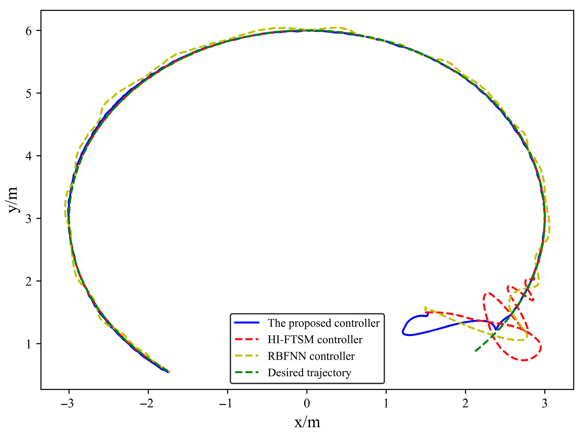
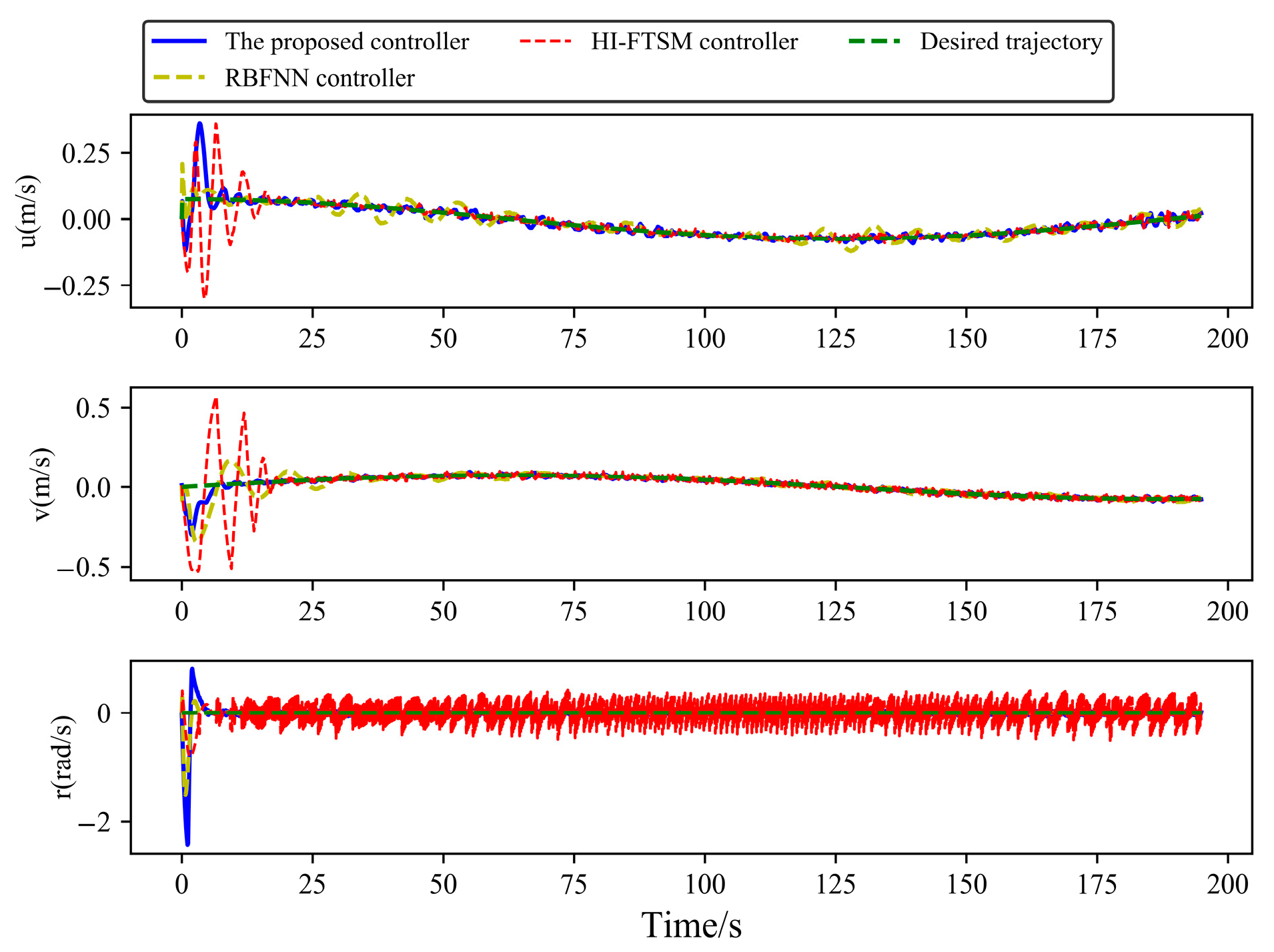
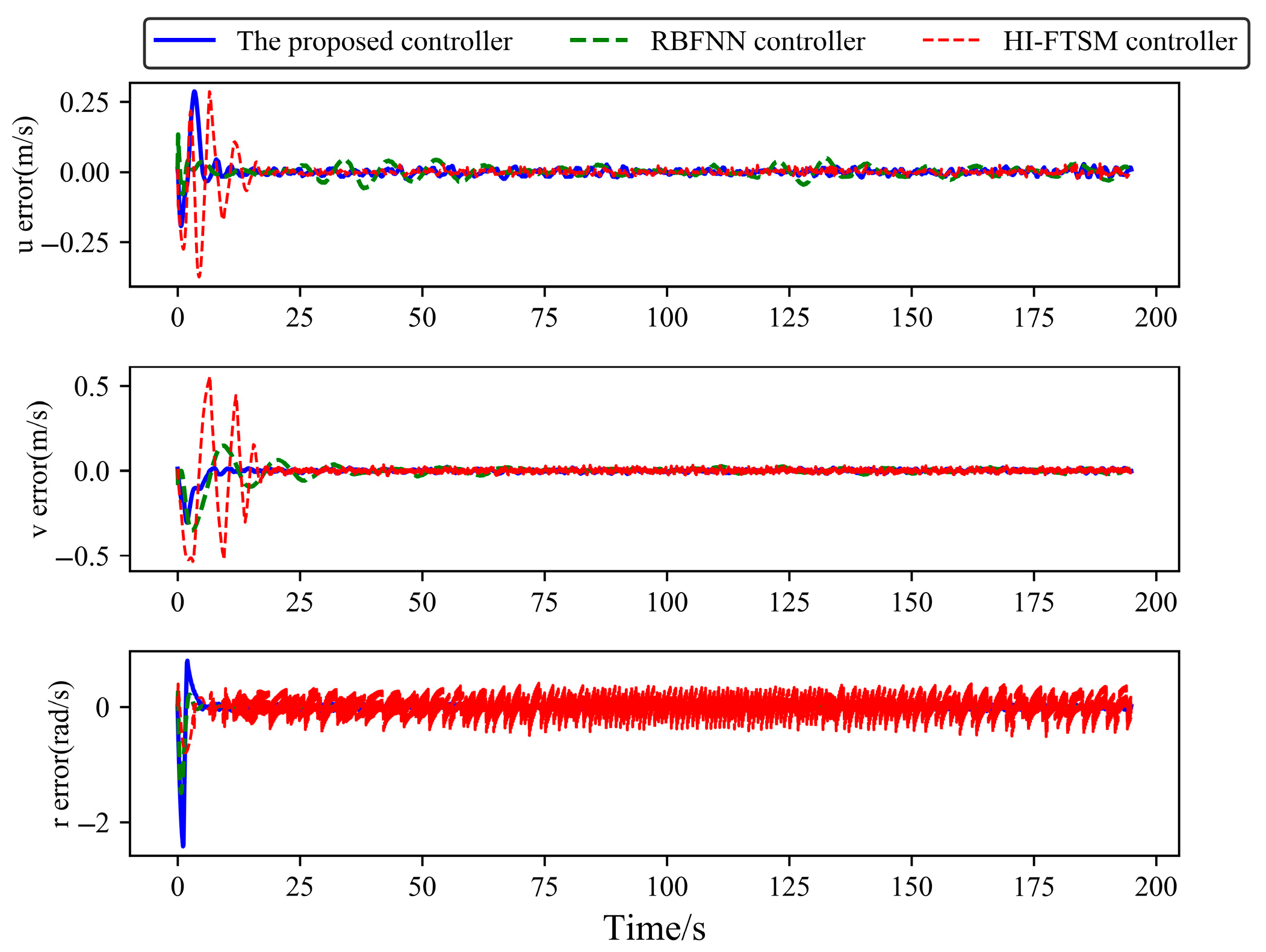
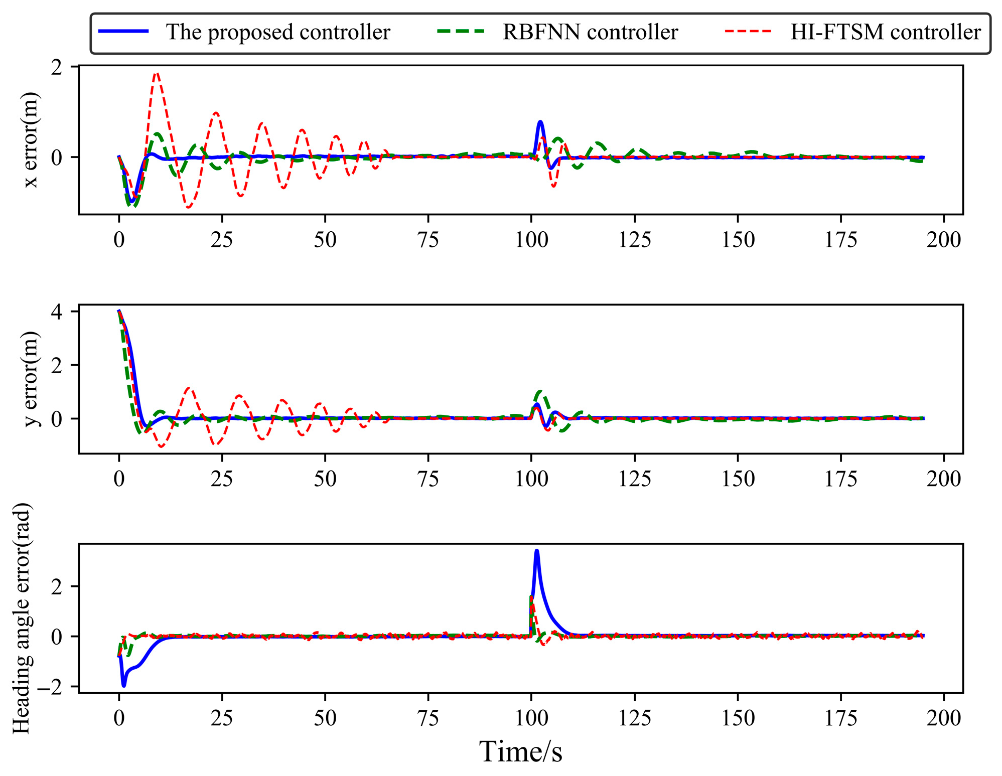
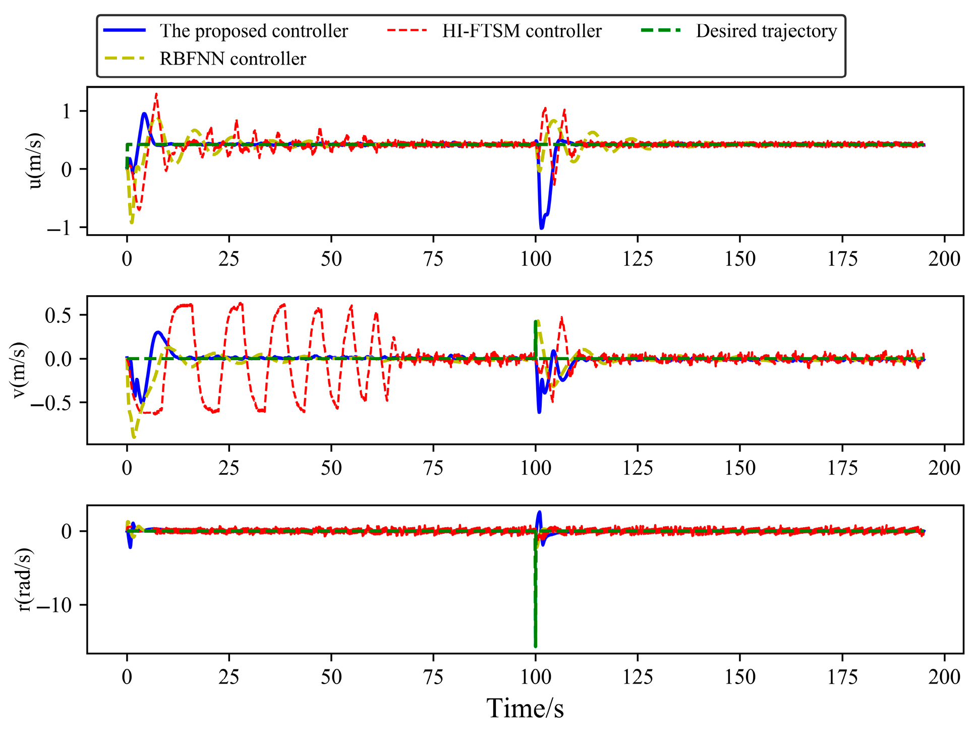
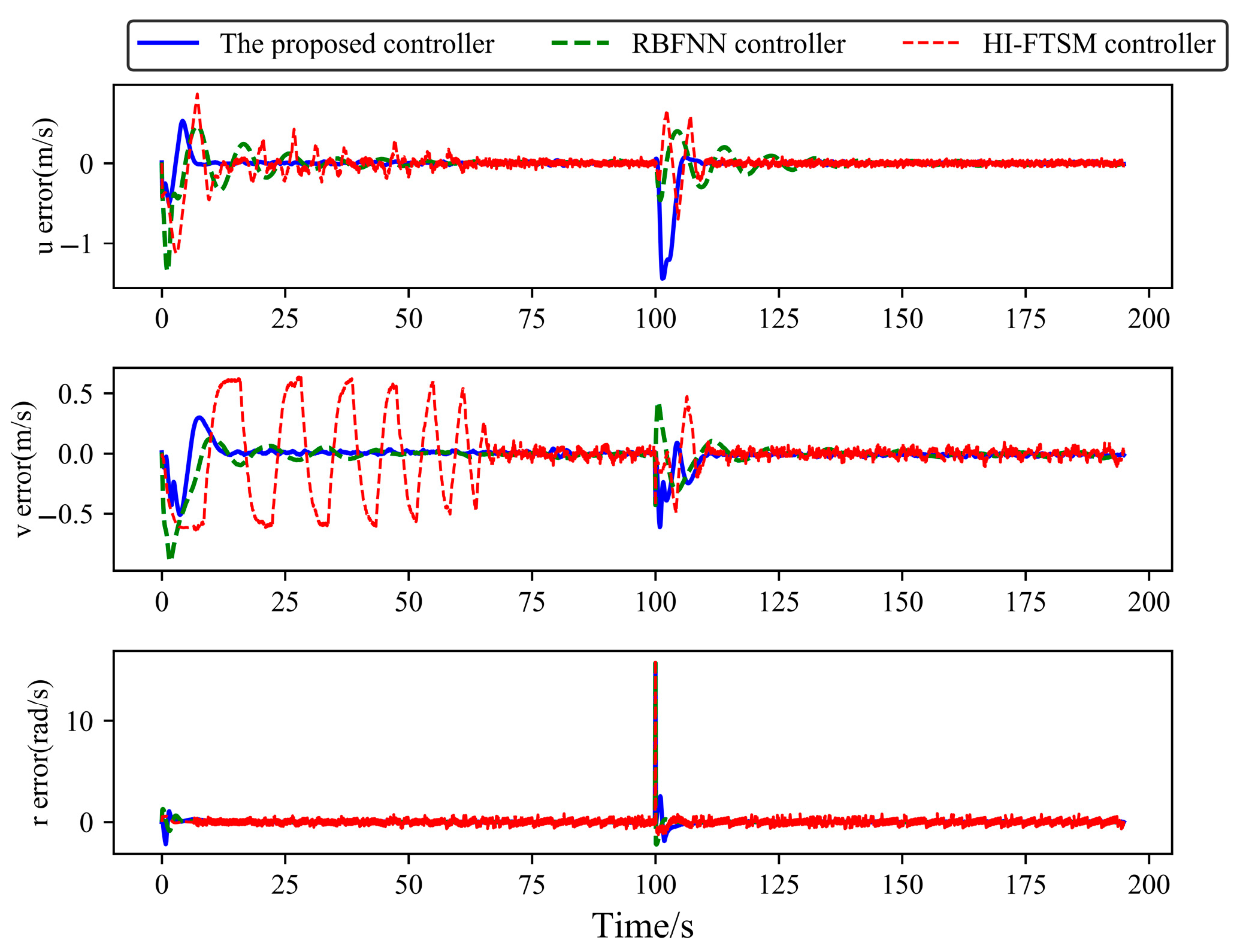
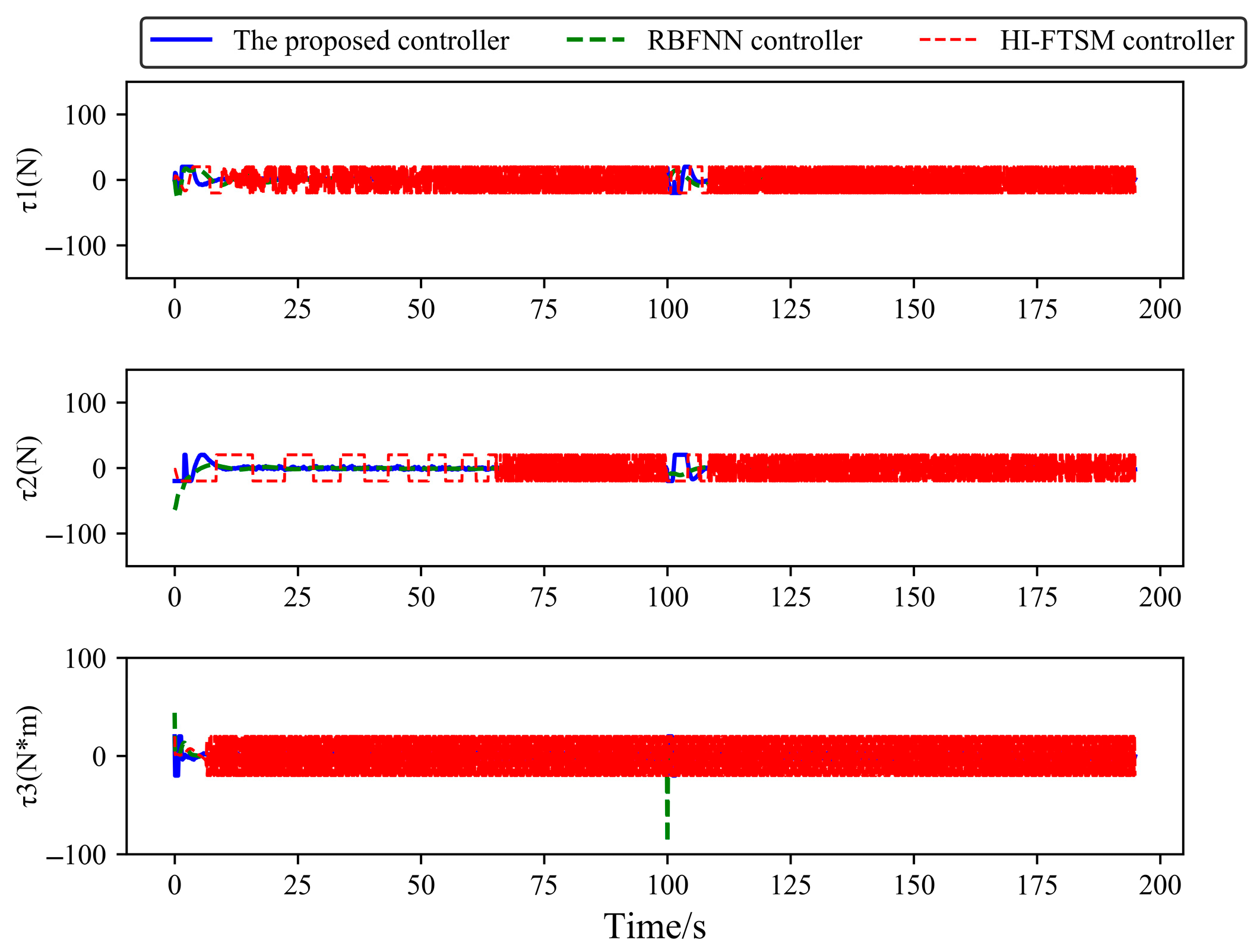
4.2. Case 1: Circular Trajectory Tracking

Case 1 verifies the performance of the controller when the controller does not consider signal delay and the USV is tracking a circular curve trajectory. In Case 1, the initial conditions of the USV are $\left[x\left(0\right),y\left(0\right),\psi \left(0\right),u\left(0\right),v\left(0\right),r\left(0\right)\right]=[1.5 \mathrm{m},1.5 \mathrm{m},120 \mathrm{d}\mathrm{e}\mathrm{g},0.1 \mathrm{m}/\mathrm{s},0.1 \mathrm{m}/\mathrm{s},0.1 \mathrm{m}/\mathrm{s}]$. The desired trajectory is as shown in Equation (49).

$$\left\{\begin{array}{l}{x}_d\left(t\right)=3sin(0.025t+{\displaystyle \frac{1}{4}}\pi )\\ y_d\left(t\right)=3(1-cos(0.025t+{\displaystyle \frac{1}{4}}\pi \left)\right)\\ {\psi }_d\left(t\right)={\displaystyle \frac{1}{4}}\pi \end{array}\right.$$

(49)

The trajectory tracking results of USVs in Case 1 are shown in Figure 3, Figure 4, Figure 5, Figure 6 and Figure 7.

From Figure 3 and Figure 4, it can be seen that when the dynamic parameters are unknown, the USV is subjected to environmental disturbances, and the USV dynamics model has unmodeled parts. Compared to the RBFNN controller and the HI-FTSM controller, the proposed controller enables the USV to track the desired trajectory, with overall smaller tracking errors in the position coordinates and heading angle. The RBFNN controller cannot make the tracking error of the USV position coordinates converge better, while the HI-FTSM controller makes the tracking error of the USVs excessively large during the initial period. From Figure 5 and Figure 6, it can be observed that the proposed controller and the RBFNN controller enable the USV’s velocity components to track the desired velocity. However, the HI-FTSM controller fails to effectively converge the tracking error of the USV’s yaw rate. From Figure 7, it can be seen that the outputs of the proposed controller and the RBFNN controller are smooth, meeting the requirements for practical applications. In contrast, the output of the HI-FTSM controller exhibits significant chattering, making it difficult to apply to real USVs. The quantitative indicators of the USV tracking error under each controller are shown in

Table 4. Quantitative analysis of tracking errors in Case 1.

Method	$\mathbf{RMS}\times {10}^2$			$\mathbf{SSE}\times {10}^2$			$\mathbf{TME}\times {10}^2$
	${\mathit{R}\mathit{M}\mathit{S}}_{\overline{\mathit{x}}}$	${\mathit{R}\mathit{M}\mathit{S}}_{\overline{\mathit{y}}}$	${\mathit{R}\mathit{M}\mathit{S}}_{\overline{\mathit{\psi }}}$	${\mathit{S}\mathit{S}\mathit{E}}_{\overline{\mathit{x}}}$	${\mathit{S}\mathit{S}\mathit{E}}_{\overline{\mathit{y}}}$	${\mathit{S}\mathit{S}\mathit{E}}_{\overline{\mathit{\psi }}}$	${\mathit{T}\mathit{M}\mathit{E}}_{\overline{\mathit{x}}}$	${\mathit{T}\mathit{M}\mathit{E}}_{\overline{\mathit{y}}}$	${\mathit{T}\mathit{M}\mathit{E}}_{\overline{\mathit{\psi }}}$
The proposed controller	8.75	5.37	10.19	2.52	1.92	1.21	67.05	62.27	130.89
RBFNN controller	9.22	9.69	7.81	3.25	4.77	2.32	67.44	66.37	133.89
HI-FTSM controller	7.88	8.48	12.40	0.17	0.18	3.34	63.31	62.13	139.98

. The average simulation time per time step and the variance of the controller output are shown in

Table 5. $D\left({\tau }_i\right)$ and simulation time in Case 1.

Method	$\mathit{D}\left({\mathit{\tau }}_1\right)$	$\mathit{D}\left({\mathit{\tau }}_2\right)$	$\mathit{D}\left({\mathit{\tau }}_3\right)$	Time Per Step (ms)
The proposed controller	6.01	5.95	6.39	2.489
RBFNN controller	3.78	4.66	1.13	0.874
HI-FTSM controller	10.39	33.77	205.95	2.400

.

As shown in Table 4 and Table 5, the proposed controller achieves a per-step computation time of 2.489 ms, meeting practical application requirements and demonstrating potential for deployment on actual USVs. Under conditions of model uncertainty and environmental disturbances, the proposed controller reduces all tracking error metrics compared to the RBFNN controller (except for ${RMS}_{\overline{\psi }}$). The proposed controller indicates superior steady-state and transient performance over the RBFNN controller.

While some metrics of the proposed controller are inferior to the HI-FTSM controller, the steady-state and transient performance of the proposed controller satisfy practical engineering requirements. Moreover, the output chattering of the proposed controller is significantly reduced compared to the HI-FTSM controller, suggesting that the proposed controller’s overall control performance surpasses that of the HI-FTSM controller.

The adaptive process of the proposed controller for unknown dynamic parameters in Case 1 is illustrated in Figure 8, Figure 9 and Figure 10.

From Figure 8, Figure 9 and Figure 10, it can be seen that as the USV trajectory tracking progresses, the proposed controller ensures that the estimation errors of the dynamic parameters remain bounded. Additionally, the estimation errors of $Y_v$, $Y_r$, $N_v$, $Y_{r\left|r\right|}$, $m_{23}$, and $m_{33}$ converge to a very small bounded region, and the estimation errors of other dynamic parameters continue to decrease. This demonstrates that the proposed controller not only ensures that the unknown dynamic parameters of the USV are SGUUB but also allows the estimation errors of some dynamic parameters to closely approximate their true values. Consequently, the robustness of the controller is significantly enhanced.

4.3. Case 2: Straight Trajectory Tracking

Case 2 verifies the performance of the controller when the controller does not consider signal delay and the USV is tracking a straight trajectory. In Case 2, the initial conditions of USVa are $\left[x\left(0\right),y\left(0\right),\psi \left(0\right),u\left(0\right),v\left(0\right),r\left(0\right)\right]=[0 \mathrm{m},4 \mathrm{m},0 \mathrm{d}\mathrm{e}\mathrm{g},0.1 \mathrm{m}/\mathrm{s},0.1 \mathrm{m}/\mathrm{s},0.1 \mathrm{m}/\mathrm{s}]$. The desired trajectory is as shown in Equation (50).

$$\left\{\begin{array}{l}{x}_d\left(t\right)=0.3t,y_d\left(t\right)=0.3t,{\psi }_d\left(t\right)={\displaystyle \frac{1}{4}}\pi t\le 100s\\ x_d\left(t\right)=0.3t+30,y_d\left(t\right)=-0.3t+30,{\psi }_d\left(t\right)=-{\displaystyle \frac{1}{4}}\pi 100s<t\le 200s\end{array}\right.$$

(50)

The trajectory tracking results of USVs in Case 3 are shown in Figure 11, Figure 12, Figure 13, Figure 14 and Figure 15.

From Figure 11, Figure 12, Figure 13, Figure 14 and Figure 15, it can be observed that, when signal delay is not considered, and applied to track the straight desired trajectory in Case 2, the proposed controller enables the position coordinates, heading angle, and velocity components to track the desired trajectory and desired velocity effectively, outperforming the HI-FTSM controller and the RBFNN controller in terms of tracking performance. This further validates the results obtained in Case 1.

4.4. Case 3: Sinusoidal Trajectory Tracking

Case 3 is designed to validate the trajectory tracking performance of the controller under signal delay conditions and to verify the effectiveness of the proposed actuator saturation scheme. Since neither the RBFNN controller nor the HI-FTSM controller incorporates a signal delay compensator, and considering that the HI-FTSM controller exhibits significant output chattering, which prevents tracking error convergence under signal delays, the comparison in Case 3 is limited to the proposed controller and the RBFNN controller. Furthermore, when signals ($\tau$,$\eta$,$\mathbf{v}$) experience delays, the RBFNN controller’s signal transmission terminal uses the input signal from the previous time step as the current time step’s input signal.

In Case 3, the initial conditions of USVs are $\left[x\left(0\right),y\left(0\right),\psi \left(0\right),u\left(0\right),v\left(0\right),r\left(0\right)\right]=[4 \mathrm{m},0 \mathrm{m},0 \mathrm{d}\mathrm{e}\mathrm{g},0.1 \mathrm{m}/\mathrm{s},0.1 \mathrm{m}/\mathrm{s},0.1 \mathrm{m}/\mathrm{s}]$. The desired trajectory is as shown in Equation (51).

$$\left\{\begin{array}{l}{x}_d\left(t\right)=1.5sin\left(0.05t\right) \\ y_d\left(t\right)=0.5t\\ {\psi }_d\left(t\right)={\displaystyle \frac{1}{4}}\pi \end{array}\right.$$

(51)

The trajectory tracking results of USVs in Case 3 are shown in Figure 16, Figure 17, Figure 18, Figure 19 and Figure 20.

As shown in Figure 16, Figure 17, Figure 18, Figure 19 and Figure 20, there are delays in both sensor-to-controller signal transmission and controller-to-actuator command transmission. The proposed controller successfully tracks the sinusoidal desired trajectory in Case 3, although the heading angle tracking error is relatively large, the position coordinates, heading angle, and velocity components can all track the desired trajectory. In contrast, the RBFNN controller demonstrates significantly larger tracking errors of position coordinates due to its lack of signal delay compensation capability. These results confirm the effectiveness of the proposed delay compensation scheme in mitigating the negative impacts of signal delays on USV trajectory tracking performance.

The results of Case 1, Case 2, and Case 3 fully demonstrate that the proposed controller exhibits strong robustness when dealing with unknown time-varying environmental disturbances, unknown dynamic parameters, unmodeled dynamics, and the sensor measurement signals and control signals have delay or loss. The proposed controller enables the USV to track the desired trajectory and desired velocity while satisfying actuator saturation constraints, and has better tracking performance than the HI-FTSM controller and the RBFNN controller.

To verify the effectiveness of the actuator saturation scheme in Equation (27) of this paper, the control scheme in which the controller proposed in this paper uses the traditional dead-zone scheme to handle the actuator saturation problem is taken as a comparison. The control law of the controller using the traditional dead-zone is as follows.

$${\tau }_0=Y_{rf}\widehat{\alpha }-K_{D}s-r_{\tau }{\Phi }_{\tau }s-k_t{\displaystyle \frac{s}{‖s‖}}+{\sigma }_q$$

(52)

In the above equation, ${\sigma }_q=\left\{\begin{array}{ll}-{\sigma }_{ai}& {\tau }_{0i}>{\tau }_{Mi}-{\sigma }_{ai}\\ {\sigma }_{ai}& {\tau }_{0i}<{-\tau }_{Mi}+{\sigma }_{ai}\end{array}\right.$, ${\sigma }_a={[4,4,4]}^T$ is the dead-zone.

For the desired trajectory shown in (51), the trajectory tracking results of the proposed controller and the dead-zone-based controller are presented in Figure 21.

The results demonstrate that the proposed controller achieves smaller overall tracking errors compared to the dead-zone approach, confirming the effectiveness of the employed actuator saturation scheme.

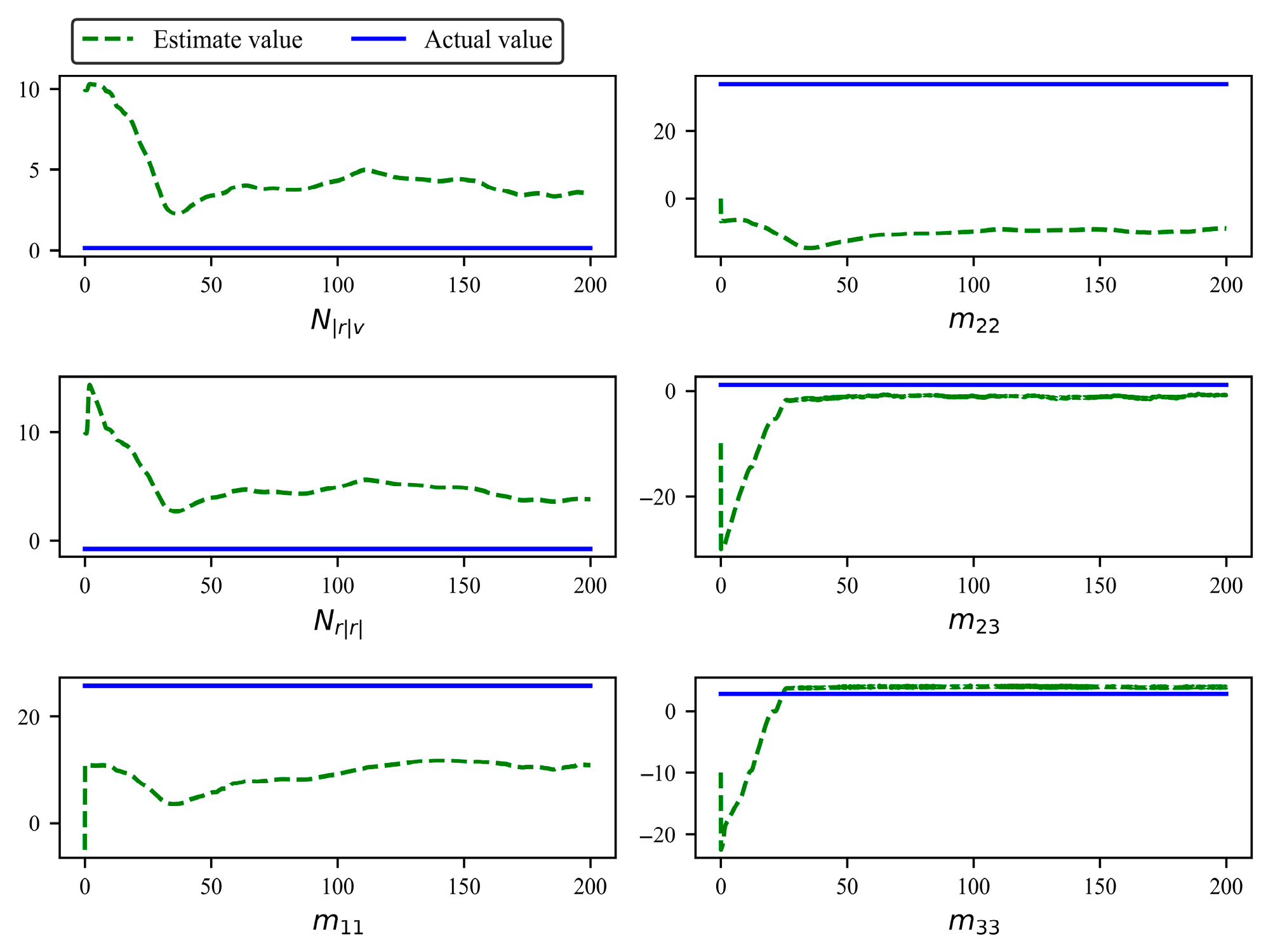
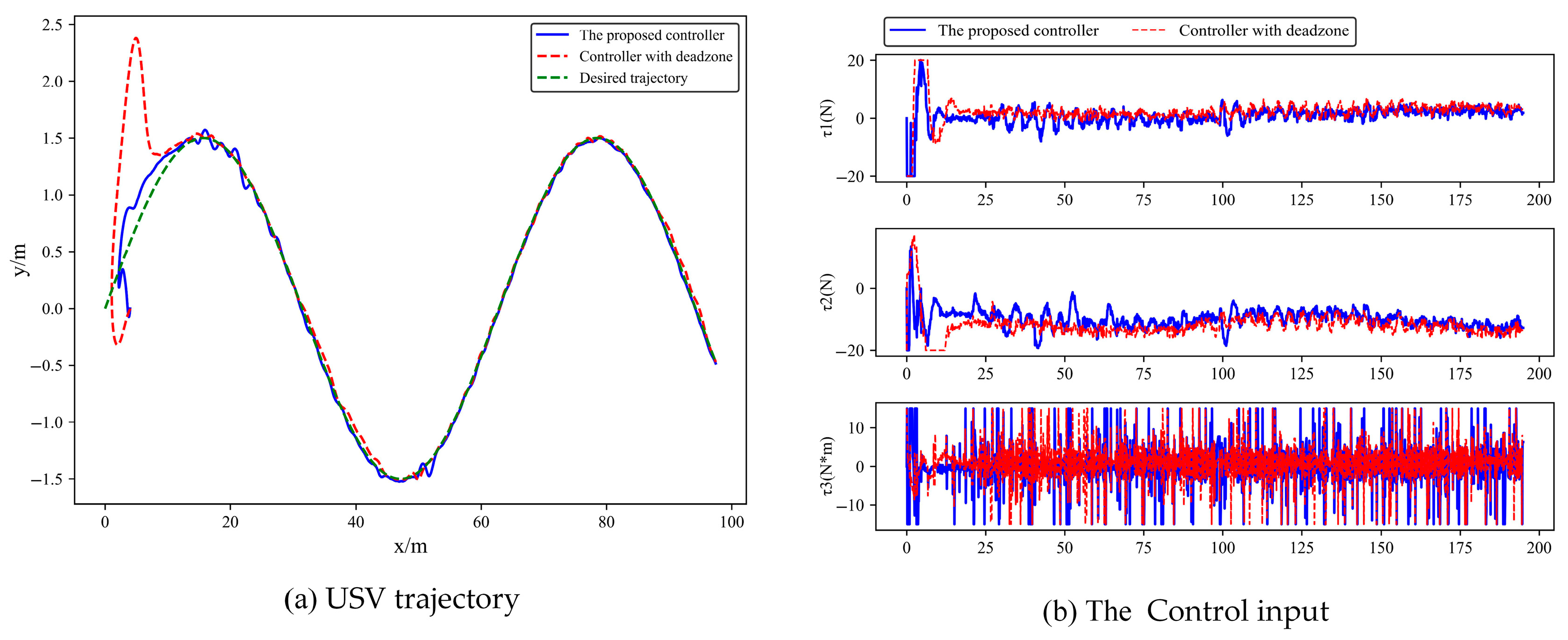
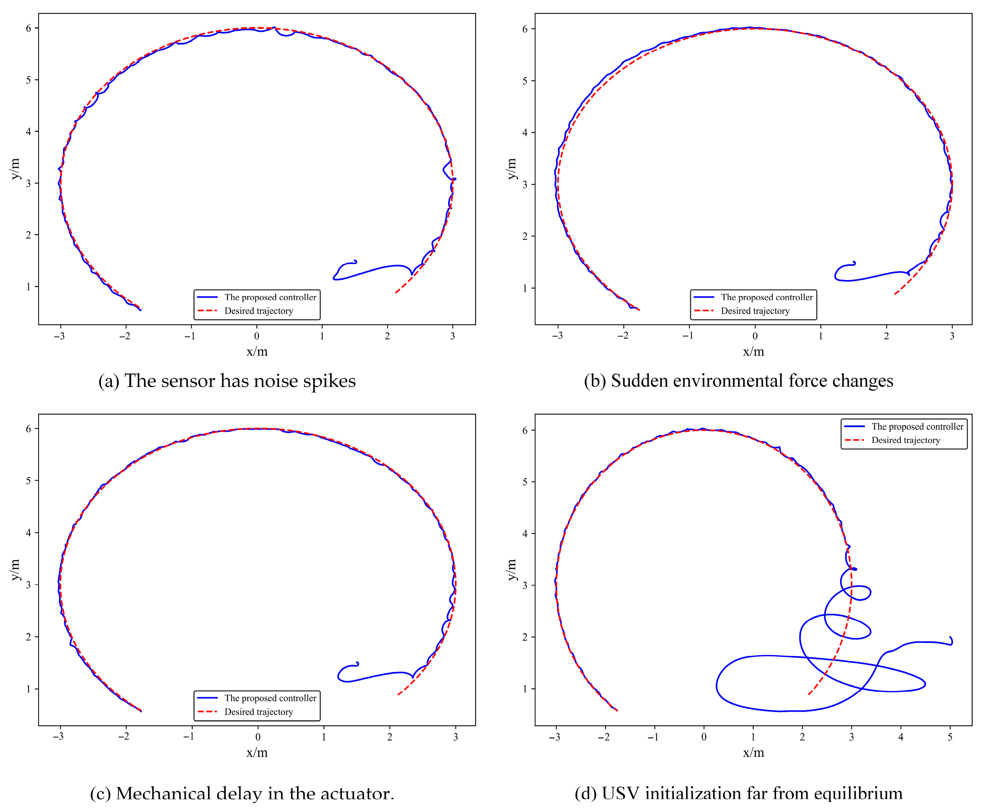
4.5. Case 4: Edge Case Exploration and Design Parameter Sensitivity and Robustness Analysis

Following references [30,31], we conducted sensitivity and robustness analyses for key controller design parameters $[{\lambda }_1,{\lambda }_2,{\lambda }_3,K_{D1},K_{D2},K_{D3},k_{\alpha },k_{\tau },r_{\tau },r_{\alpha },l]$. The analysis procedure is as follows:

(1)

For the target parameter ${\lambda }_1$, select 9 values [${\lambda }_{11},\dots , {\lambda }_{19}$] within its reasonable range.

(2)

Fix ${\lambda }_1$ = ${\lambda }_{11}$ while keeping other parameters at Table 3 values. Using desired trajectory (49), simulate 20 USV tracking voyages (1000 steps each) with: sensor noise (methodology as before); environmental disturbances (methodology as before); unmodeled dynamics via randomized scaling factor k = 0.2~0.4 applied to $∆M=k{M}_0, ∆D\left(\mathbf{v}\right)=k{D}_0\left(\mathbf{v}\right)$, and $∆C\left(\mathbf{v}\right)=k{C}_0\left(\mathbf{v}\right)$ to simulate the unmodeled part in the USV dynamic model under this tracking voyage. Record performance metrics ${RMS}_e={RMS}_{\overline{x}}+{RMS}_{\overline{y}}$, and generate boxplots based on ${RMS}_e$ to evaluate robustness at ${\lambda }_{11}$.

(3)

Repeat step 2 for ${\lambda }_{12}$… ${\lambda }_{19}$ to obtain sensitivity trends.

(4)

Iterate for other design parameters.

The results of the robustness and sensitivity analysis of the main design parameters are shown in Figure 22.

As can be seen from the above figure, the design parameters of this paper have certain robustness. When the values of the design parameters are in a reasonable range, they are not sensitive to the trajectory tracking results. The values of each design parameter in Table 3 are reasonable.

To analyze the performance of the controller proposed in this paper under extreme conditions, taking Equation (49) as the desired trajectory, considering model uncertainty, environmental disturbances, the following edge cases are analyzed.

(a)

Sensor noise spikes:

In the sensor collects signals $[x,y,\psi ,u,v,r]$, Gaussian white noise (σ² = 0.001) is superimposed with intermittent spikes occurring every 100 time steps, where spikes followed N (0,0.01).

(b)

Sudden environmental force changes:

Every 100 time steps, the USV experienced a disturbance force equal to 3 times of the nominal environmental force.

(c)

Actuator mechanical delay:

The actuator experiences a mechanical delay every 50 time steps, causing the control force output by the actuator at that moment to be the same as that of the previous moment.

(d)

Off-equilibrium initialization:

For trajectory (49), USV initial conditions are: $\left[x\left(0\right),y\left(0\right),\psi \left(0\right),u\left(0\right),v\left(0\right),r\left(0\right)\right]=[5 \mathrm{m},2\mathrm{m},120 \mathrm{d}\mathrm{e}\mathrm{g},0.1 \mathrm{m}/\mathrm{s},0.1 \mathrm{m}/\mathrm{s},0.1 \mathrm{m}/\mathrm{s}]$.

Under the above various edge cases, the trajectory tracking results of the controller designed in this paper are shown in Figure 23.

As can be seen from the above figure, when the controller designed in this paper faces various extreme conditions, although the tracking error increases to some extent, it can still enable the USV to track the desired trajectory. It can be seen that the controller designed in this paper has good robustness.

5. Conclusions

This paper addresses the trajectory tracking problem of USVs under unknown time-varying environmental disturbances, unknown dynamic parameters, unmodeled dynamics, and actuator saturation constraints by designing a robust neural adaptive controller (RNA controller). First, based on the USV dynamic model, which is linearly parameterized, an adaptive law for the unknown dynamic parameters was designed through a series of filtering operations. Second, a finite-time auxiliary variable was designed to handle actuator saturation. The unmodeled dynamics of USVs were approximated using RBF-NNs, and the robust neural damping technique was introduced to design a robust damping term to compensate for the unmodeled dynamics and environmental disturbances. Based on the above design methods, the RNA controller was developed using Lyapunov theory and adaptive control techniques. Subsequently, the convergence of all signals in the closed-loop system was proven based on Lyapunov theory. And signal delay compensators were designed to compensate for the negative impact on the USV trajectory tracking when there is a delay in the system input signal. Finally, numerical simulation experiments were conducted, and the results demonstrated that the RNA controller exhibits strong robustness in the presence of environmental disturbances and model uncertainties.

Applying the proposed controller to a real USV is the next research direction of this paper.

References

1. Qu, Y.; Cai, L. Simultaneous planning and executing trajectory tracking control for underactuated unmanned surface vehicles from theory to practice. Ocean. Eng. 2023, 270, 113665. [Google Scholar] [CrossRef]
2. Sui, B.; Zhang, J.; Liu, Z. Prescribed-time dynamic positioning control for USV with lumped disturbances, thruster saturation and prescribed performance constraints. Remote Sens. 2024, 16, 4142. [Google Scholar] [CrossRef]
3. Zheng, S.; Su, Y.; Zhuang, J.; Tang, Y.; Yi, G. Fixed-time path-following-based underactuated unmanned surface vehicle dynamic positioning control. J. Mar. Sci. Eng. 2024, 12, 551. [Google Scholar] [CrossRef]
4. Yuan, W.; Rui, X. Deep reinforcement learning-based controller for dynamic positioning of an unmanned surface vehicle. Comput. Electr. Eng. 2023, 110, 108858. [Google Scholar] [CrossRef]
5. Liu, Z.; Song, S.; Yuan, S.; Ma, Y.; Yao, Z. ALOS-based USV path-following control with obstacle avoidance strategy. J. Mar. Sci. Eng. 2022, 10, 1203. [Google Scholar] [CrossRef]
6. Lin, M.; Zhang, Z.; Pang, Y.; Lin, H.; Ji, Q. Underactuated USV path following mechanism based on the cascade method. Sci. Rep. 2022, 12, 1461. [Google Scholar] [CrossRef] [PubMed]
7. Zhang, G.; Lin, C.; Li, J.; Zhang, W. Composite anti-disturbance path following control for the underactuated surface vessel under actuator faults. Nonlinear Dyn. 2024, 113, 3579–3592. [Google Scholar] [CrossRef]
8. Wu, C.; Yu, W.; Liao, W.; Ouyang, H. Deep reinforcement learning with intrinsic curiosity module based trajectory tracking control for USV. Ocean. Eng. 2024, 308, 118342. [Google Scholar] [CrossRef]
9. Xu, D.; Liu, Z.; Song, J.; Zhou, X. Finite time trajectory tracking with full-state feedback of underactuated unmanned surface vessel based on nonsingular fast terminal sliding mode. J. Mar. Sci. Eng. 2022, 10, 1845. [Google Scholar] [CrossRef]
10. Xiong, Y.; Zhu, H.; Pan, L.; Wang, J. Research on intelligent trajectory control method of water quality testing unmanned surface vessel. J. Mar. Sci. Eng. 2022, 10, 1252. [Google Scholar] [CrossRef]
11. Wang, Y.; Shen, C.; Chen, H. Event-triggered trajectory tracking control for USV with prescribed performance and time delay based on differential flatness. Meas. Control 2024, 57, 1023–1034. [Google Scholar] [CrossRef]
12. Yuan, S.; Liu, Z.; Sun, Y.; Wang, Z.; Zheng, L. An event-triggered trajectory planning and tracking scheme for automatic berthing of unmanned surface vessel. Ocean. Eng. 2023, 273, 113964. [Google Scholar] [CrossRef]
13. Souissi, S.; Boukattaya, M. Time-varying nonsingular terminal sliding mode control of autonomous surface vehicle with predefined convergence time. Ocean. Eng. 2022, 263, 112264. [Google Scholar] [CrossRef]
14. Zheng, Y.; Tao, J.; Hartikainen, J.; Duan, F.; Sun, H.; Sun, M.; Sun, Q.; Zeng, X.; Chen, Z.; Xie, G. DDPG based LADRC trajectory tracking control for underactuated unmanned ship under environmental disturbances. Ocean. Eng. 2023, 271, 113667. [Google Scholar] [CrossRef]
15. Liu, W.; Ye, H.; Yang, X. Model-Free Adaptive Sliding Mode Control Method for Unmanned Surface Vehicle Course Control. J. Mar. Sci. Eng. 2023, 11, 17. [Google Scholar] [CrossRef]
16. Souissi, S.; Boukattaya, M.; Damak, T.; Nejim, S. Adaptive control for fully-actuated autonomous surface vehicle with uncertain model and unknown ocean currents. Ocean. Eng. 2020, 217, 108147. [Google Scholar] [CrossRef]
17. Xiong, Y.; Wang, X.; Zhou, S. Online Interactive Identification Method Based on ESO Disturbance Estimation for Motion Model of Double Propeller Propulsion Unmanned Surface Vehicle. Control. Theory Technol. 2024, 22, 292–314. [Google Scholar] [CrossRef]
18. Wang, H.; Luo, Q.; Li, N.; Zheng, W. Data-Driven Model Free Formation Control for Multi-USV System in Complex Marine Environments. Int. J. Control. Autom. Syst. 2022, 20, 3666–3677. [Google Scholar] [CrossRef]
19. He, Z.; Fan, Y.; Wang, G.; Mu, D. Cooperative trajectory tracking control of MUSVs with periodic relative threshold event-triggered mechanism and safe distance. Ocean. Eng. 2022, 269, 113541. [Google Scholar] [CrossRef]
20. Mu, D.; Li, L.; Wang, G.; Fan, Y.; Zhao, Y.; Sun, X. State constrained control strategy for unmanned surface vehicle trajectory tracking based on improved barrier Lyapunov function. Ocean. Eng. 2023, 286, 114276. [Google Scholar] [CrossRef]
21. Zhang, G.; Dong, X.; Liu, J.; Zhang, X. Nussbaum-type function based robust neural event-triggered control of unmanned surface vehicle subject to cyber and physical attacks. Ocean. Eng. 2023, 270, 113664. [Google Scholar] [CrossRef]
22. Zhang, C.; Wang, C.; Wang, J.; Li, C. Neuro-adaptive trajectory tracking control of underactuated autonomous surface vehicles with high-gain observer. Appl. Ocean. Res. 2020, 97, 102051. [Google Scholar] [CrossRef]
23. Meng, Y.; Ye, H.; Xiang, Z.; Yang, X.; Zhang, H. An adaptive internal model control approach for unmanned surface vehicle based on bidirectional long short-term memory neural network: Implementation and field testing. Mechatronics 2024, 99, 103145. [Google Scholar] [CrossRef]
24. Fossen, T.I. Handbook of Marine Craft Hydrodynamics and Motion Control; Wiley: Hoboken, NJ, USA, 2011. [Google Scholar] [CrossRef]
25. Yan, Z.; Feng, W.; Wang, H. Adaptive surge control of variable-mass unmanned surface vehicle based on sliding mode observation. Ocean. Eng. 2022, 269, 113576. [Google Scholar] [CrossRef]
26. Li, S.; Xu, C.; Liu, J.; Han, B. Data-driven docking control of autonomous double-ended ferries based on iterative learning model predictive control. Ocean. Eng. 2023, 273, 113994. [Google Scholar] [CrossRef]
27. Huang, J.; Xu, D.; Li, Y.; Ma, Y. Near-optimal tracking control of partially unknown discrete-time nonlinear systems based on radial basis function neural network. Mathematics 2024, 12, 1146. [Google Scholar] [CrossRef]
28. Li, G.; Li, W.; Hildre, H.P.; Zhang, H. Online learning control of surface vessel for fine trajectory tracking. J. Mar. Sci. Technol. 2015, 21, 251–260. [Google Scholar] [CrossRef]
29. Yao, Q. Adaptive finite-time sliding mode control design for finite-time fault-tolerant trajectory tracking control of marine vehicles with input saturation. J. Frankl. Inst. 2020, 357, 13593–13619. [Google Scholar] [CrossRef]
30. Owais, M.; Moussa, G.S. Global sensitivity analysis for studying hot-mix asphalt dynamic modulus parameters. Constr. Build. Mater. 2023, 413, 15. [Google Scholar] [CrossRef]
31. Idriss, L.K.; Owais, M. Global sensitivity analysis for seismic performance of shear wall with high-strength steel bars and recycled aggregate concrete. Constr. Build. Mater. 2023, 411, 17. [Google Scholar] [CrossRef]
Figure 1. USV motion coordinate system.
Jmse 13 01341 g001
Figure 2. Controller calculation block diagram.
Jmse 13 01341 g002
Figure 3. USV trajectory in Case 1.
Jmse 13 01341 g003
Figure 4. Tracking errors of USV (x, y) coordinates and heading angles in Case 1.
Jmse 13 01341 g004
Figure 5. Velocity components of USVs in Case 1.
Jmse 13 01341 g005
Figure 6. Tracking error of USV velocity components in Case 1.
Jmse 13 01341 g006
Figure 7. Control input of USVs in Case 1.
Jmse 13 01341 g007
Figure 8. Part 1: dynamic parameters adaptation process in Case 1.
Jmse 13 01341 g008
Figure 9. Part 2: dynamic parameters adaptation process in Case 1.
Jmse 13 01341 g009
Figure 10. Part 3: dynamic parameters adaptation process in Case 1.
Jmse 13 01341 g010
Figure 11. USV trajectory in Case 2.
Jmse 13 01341 g011
Figure 12. Tracking errors of USV (x, y) coordinates and heading angles in Case 2.
Jmse 13 01341 g012
Figure 13. Velocity components of USVs in Case 2.
Jmse 13 01341 g013
Figure 14. Tracking error of USV velocity components in Case 2.
Jmse 13 01341 g014
Figure 15. Control input of USVs in Case 2.
Jmse 13 01341 g015
Figure 16. USV trajectory in Case 3.
Jmse 13 01341 g016
Figure 17. Tracking errors of USV (x, y) coordinates and heading angles in Case 3.
Jmse 13 01341 g017
Figure 18. Velocity components of USVs in Case 3.
Jmse 13 01341 g018
Figure 19. Tracking error of USV velocity components in Case 3.
Jmse 13 01341 g019
Figure 20. Control input of USVs in Case 3.
Jmse 13 01341 g020
Figure 21. Actuator saturation scheme verification.
Jmse 13 01341 g021
Figure 22. The robustness and sensitivity analysis of the main design parameters.
Jmse 13 01341 g022
Figure 23. Trajectory tracking in edge cases.
Jmse 13 01341 g023