Temperature Prediction and Fault Warning of High-Speed Shaft of Wind Turbine Gearbox Based on Hybrid Deep Learning Model

Abstract

Gearbox failure represents one of the most time-consuming maintenance challenges in wind turbine operations. Abnormal temperature variations in the gearbox high-speed shaft (GHSS) serve as reliable indicators of potential faults. This study proposes a Spatio-Temporal Attentive (STA) synergistic architecture for GHSS fault detection and early warning by utilizing the in situ monitoring data from a wind farm. This comprehensive architecture involves five modules: data preprocessing, multi-dimensional spatial feature extraction, temporal dependency modeling, global relationship learning, and hyperparameter optimization. It was achieved by using real-time monitoring data to predict the GHSS temperature in 10 min, with an accuracy of 1 °C. Compared to the long short-term memory (LSTM) and convolutional neural network and LSTM hybrid models, the STA architecture reduces the root mean square error of the prediction by approximately 37% and 13%, respectively. Furthermore, the architecture establishes a normal operating condition model and provides benchmark eigenvalues for subsequent fault warnings. The model was validated to issue early warnings up to seven hours before the fault alert is triggered by the supervisory control and data acquisition system of the wind turbine. By offering reliable, cost-effective prognostics without additional hardware, this approach significantly improves wind turbine health management and fault prevention.

1. Introduction

As wind power expands globally, aging turbines are failing more often [1]. Gearboxes, as wind turbines’ critical transmission component, not only account for the most significant downtime (exceeding 20% of total failure-related outages [2]) but also require high maintenance costs [3,4]. The health status of the gearbox directly affects the overall system reliability and power generation efficiency. Among all gearbox components, the gearbox high-speed shaft (GHSS) is especially vulnerable. Common failure modes of wind turbine gearbox high-speed shafts include fatigue fracture (often initiating at stress concentrators like shoulders or keyways due to cyclic bending/torsional loads), shaft damage induced by bearing failure (causing wear, bending, or micro-fretting at bearing seats), various wear mechanisms (abrasive, adhesive, or fretting wear from contamination or lubrication issues), overload fracture/bending from extreme transient events, and corrosion or corrosion-fatigue accelerated by moisture ingress [5]. The temperature anomaly of the GHSS is a critical early indicator of these potential failures [6].

The supervisory control and data acquisition (SCADA) system, widely used for wind turbine monitoring, tracks multiple variables, including the gearbox high-speed shaft temperature (GHSST). When the GHSST surpasses a set threshold, the SCADA system triggers alarms and shutdowns. However, the GHSST fluctuates significantly due to complex factors like environmental conditions and operational states. Fixed thresholds alone cannot reliably detect GHSS anomalies. For example, a gearbox fault under low ambient temperatures may delay the GHSST from reaching the threshold. During this delay, the turbine keeps operating with undetected faults, risking further structural damage. Thus, developing a method for timely GHSS fault detection and early warnings across diverse conditions is critical.

The structural analysis and failure investigations of GHSS can be performed using various approaches. Typical offline methods include computational fluid dynamics simulations [7], finite element analysis [8], and thermal network modeling [9]. These offline methods are especially critical during the wind turbine design phases. Once the turbines are deployed, monitoring data becomes an essential tool for failure detection and fault warnings. Fault diagnosis based on monitoring signals generally falls into two categories: traditional signal analysis and data-driven approaches. Traditional signal analysis has evolved over decades, yielding various fault detection and warning methods [10]. However, these methods typically rely on one or several following assumptions: well-defined physical mechanisms, relatively stable boundary conditions, low stochasticity, and low-dimensional data spaces [11]. In this study, gearbox damages result from multiple factors with ambiguous physical mechanisms. The SCADA system’s long sampling periods (usually over 5 min) are inadequate for capturing transient damage processes. Furthermore, wind turbines operate under continuously varying environmental conditions and dynamic states, causing unstable boundary conditions and significant stochasticity. Additionally, the GHSST is correlated with multiple variables from the SCADA system. Multi-dimensional data are necessary for a comprehensive diagnosis. Given these constraints, it is worth investigating data-driven methods for advancing GHSS fault diagnosis and early warning.

Machine learning methods excel at extracting latent patterns from high-dimensional SCADA data [12,13,14]. The current research predominantly focuses on fault diagnosis (i.e., fault classification and localization), while fault prediction and early warning are relatively limited [15,16,17]. Traditional machine learning methods perform well in fault classification. However, these methods rely heavily on manual feature engineering, making them less adaptable to dynamic operating conditions. Deep learning, leveraging hierarchical nonlinear transformations, significantly enhances detection accuracy [18]. Shao et al. proposed a novel deep-autoencoder-based fault diagnosis method [19]. It integrates the maximum correntropy criterion for robust feature learning under noisy conditions and the artificial fish swarm algorithm for adaptive parameter optimization. Experimental validation demonstrated its superior effectiveness in gearbox and bearing fault detection. Other fault diagnosis models include convolutional neural networks (CNNs) [20], long short-term memory networks (LSTM) [21], extreme gradient boosting (XGBoost) [22], gated recurrent units [23], and stacked models [24]. Nonetheless, these approaches primarily focus on classification tasks, with limited research on fault prediction.

Fault prediction infers the future state evolution from historical data, offering greater engineering value than passive diagnostics [25]. Model-based methods rely on a residual analysis against normal operational baselines to generate early alerts [26,27]. Model selection is critical, determining generalization capabilities from historical to future states. Common approaches include artificial neural networks (ANNs) [28] and principal component analysis (PCA) [29]—ANN achieves a 44.4% cost reduction in wind farm maintenance, while PCA attains sub-1% false alarm rates in sensor networks. However, their limitations persist: ANN overlooks mechanical interdependencies and environmental dynamics, while PCA struggles with nonlinear sensor responses and real-time demands. Rezamand et al. reviewed the adaptive-network-based fuzzy inference system (ANFIS), recurrent neural network (RNN) variants, and extreme learning machines for the remaining useful life prediction [30], finding hybrid methods (e.g., ANFIS with particle filtering or Bayesian algorithms) superior for accuracy under variable conditions. Time-series regression models of temperature parameters effectively assess turbine health [31]. XGBoost and LightGBM are two emerging fault detection methods. Studies demonstrate their superiority over traditional deep learning approaches due to their robustness and computational efficiency as well as their abilities to work with real-time data [32,33].

Selecting appropriate indicators proves critical for fault prediction under constantly shifting boundary conditions. For example, fixed-threshold temperature methods lack adaptability to operational variability and require repeated calibration across turbine fleets, hindering generalizability [34]. Similarly, RMSE-based warnings rely solely on monolithic metrics that overlook data dependencies, triggering false alarms or missed detections [35]. Bangalore et al. [36] demonstrate the use of the Mahalanobis distance as a dynamic threshold alternative that outperforms traditional methods. Nevertheless, this approach assumes multivariate normality—an invalid premise for gearbox temperature data during sudden operational shifts where bimodal distributions cause erroneous anomaly probabilities. Its static covariance matrix also fails to track the system evolution over time.

The challenges for GHSS fault prediction in engineering applications can be summarized as follows:

• Noise sensitivity: Raw SCADA data contains multi-source noise, such as shutdown periods and power-limiting operations. Existing data-cleaning methods lack the adaptability to heterogeneous noise, adversely affecting model performance [37,38].
• Insufficient spatio-temporal coupling modeling: The low-frequency nature of SCADA data results in the inadequate extraction of cross-variable interactions and long-term dependencies. Additionally, determining optimal network hyperparameters remains challenging, and some studies fail to model normal operating conditions effectively.
• Lack of dynamic adaptability in alarm indicators: The fixed-threshold alarm mechanism in the SCADA system struggles to detect early-stage temperature accumulation leading to faults. Moreover, most existing fault-warning methods rely on single statistical error metrics as thresholds, neglecting dynamic data correlations. This results in poor adaptability and limited generalization across different operational scenarios.

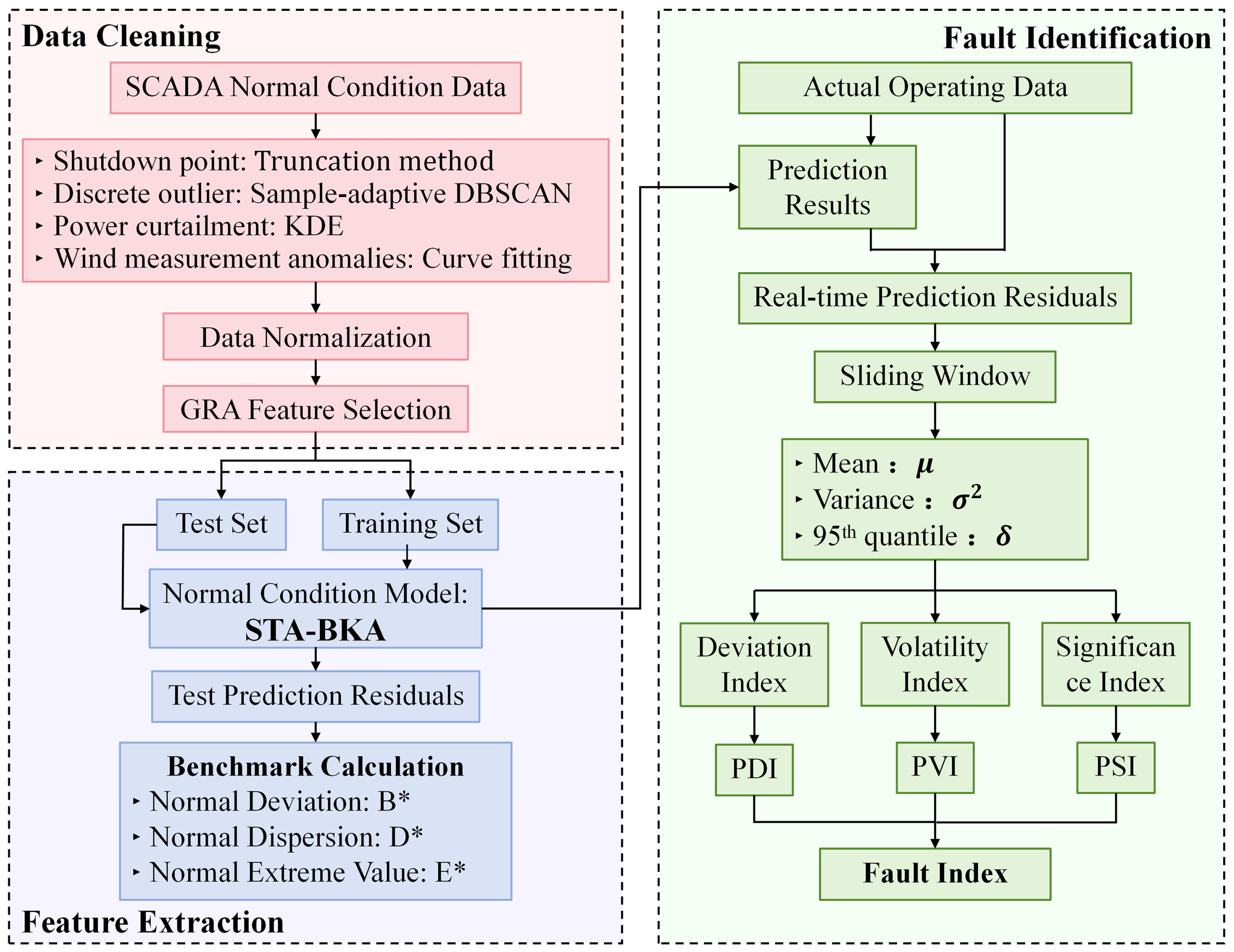
To overcome the aforementioned challenges and enhance wind farms’ maintenance, a comprehensive architecture is proposed, including data preprocessing, multi-dimensional spatial feature extraction, temporal dependency modeling, global relationship learning, and hyperparameter optimization. The remainder of the paper is organized as follows: Section 2 introduces the proposed method, including methods for multidimensional data cleaning, the composition of the improved hybrid deep learning model, and the principles of fault early warning. Section 3 presents the preprocessing of SCADA data from actual wind turbine operations, including data cleaning algorithms, normalization, and steps for feature extraction. Section 4 details the mathematical formulation of the proposed hybrid deep learning architecture. 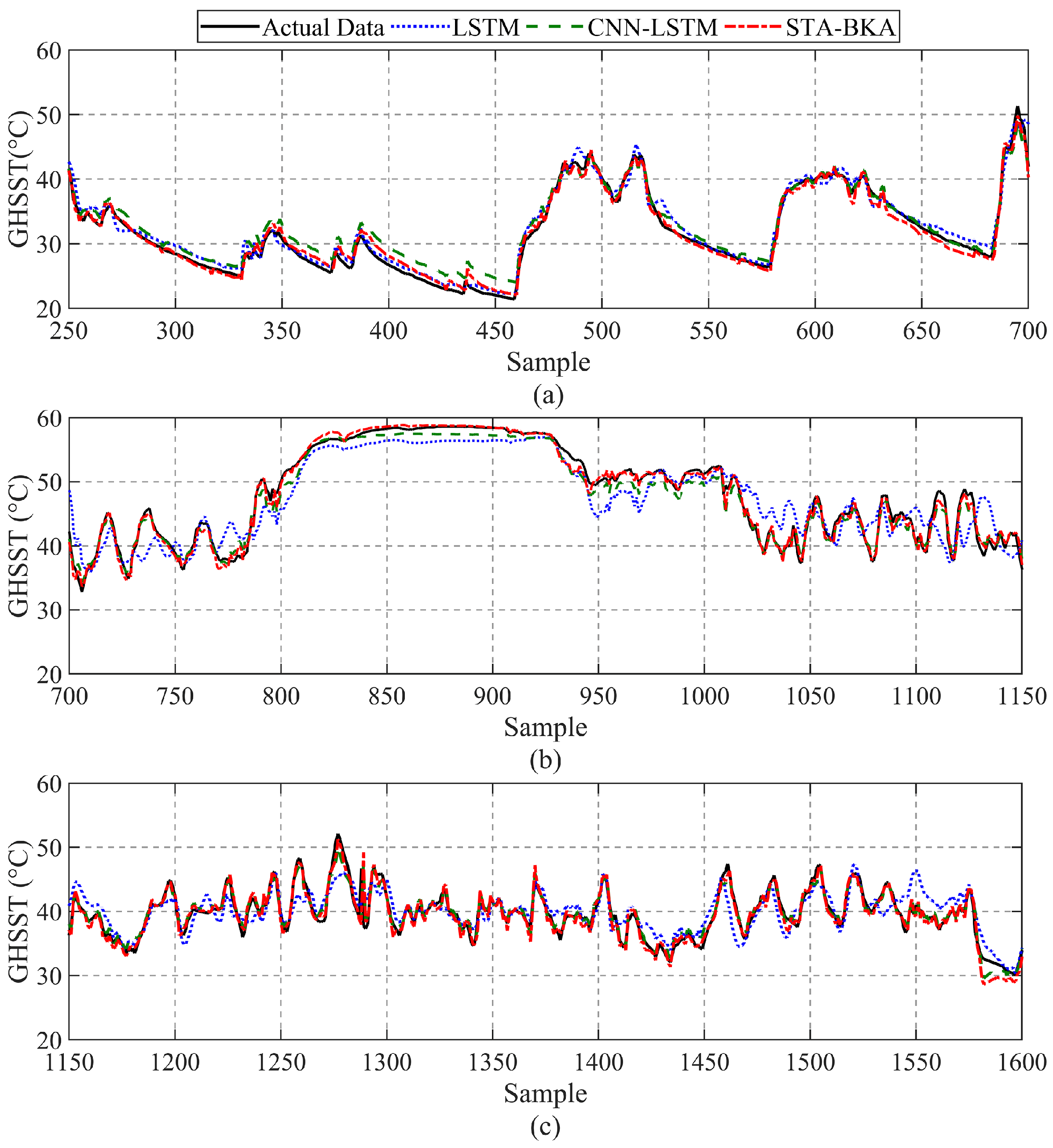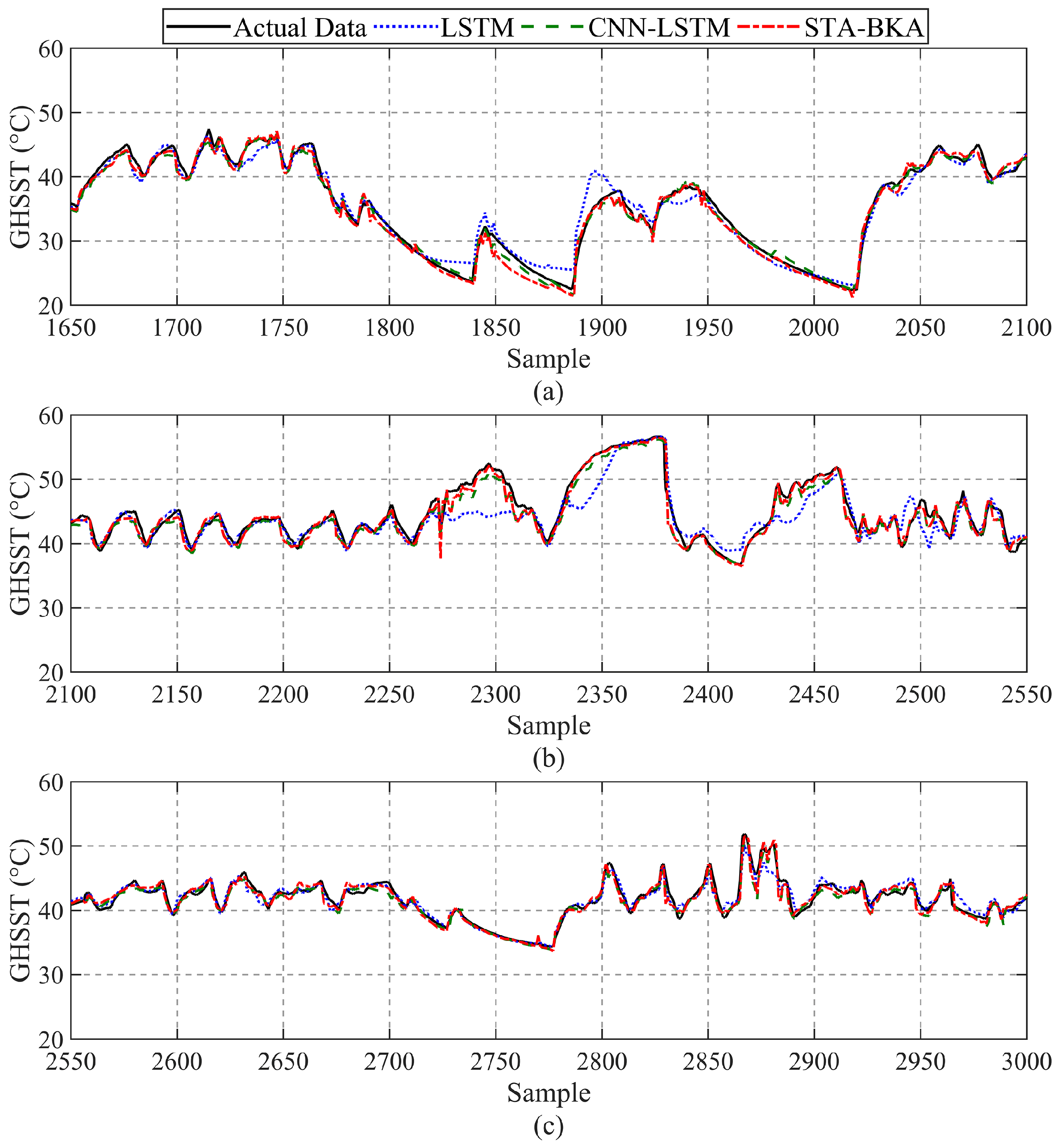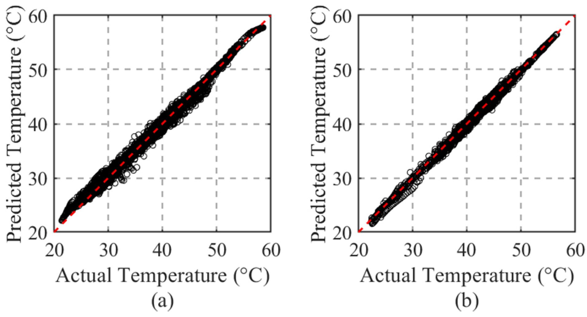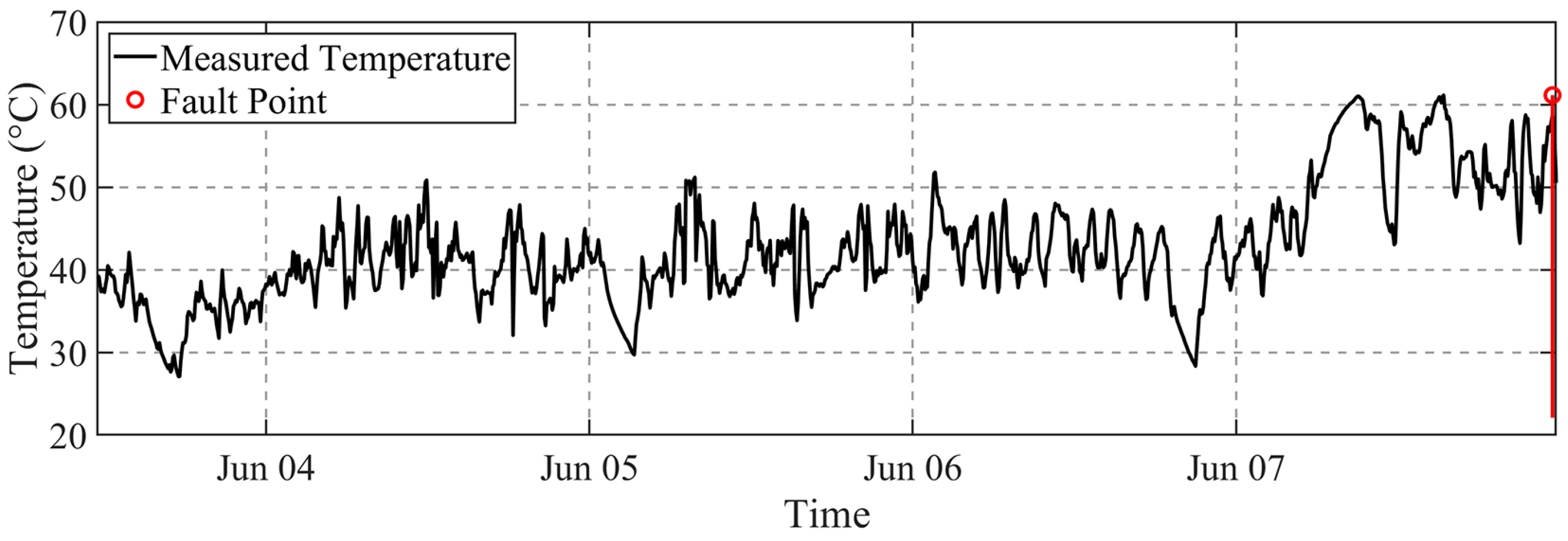Section 5 applies the model to predict the GHSST in real wind turbine operation cases, comparing the operational data preceding failures with fault logs to generate warnings via fault indices. Finally, Section 6 concludes the paper.

2. Method

Gearbox failures cause the longest downtime for wind turbines and are costly to repair [3]. The GHSS, as the most stressed component in wind turbine drivetrains, plays a critical role in operational safety. This study adopts a systematic methodology beginning with rigorous data preprocessing. We meticulously categorize anomalous data types by distributional characteristics and root causes, implementing a comprehensive multidimensional anomaly detection and cleansing strategy. Then, we develop an advanced hybrid deep learning architecture, specifically designed for GHSST prediction in wind turbine gearboxes. The model’s hyperparameters are optimized using the black-winged kite algorithm (BKA), ensuring optimal predictive performance. Finally, fault warnings are generated by applying the temperature prediction model to normal operational data.

2.1. Overview of Article Framework

The proposed method consists of three core modules:

• Multidimensional data cleansing: To address the heterogeneity of noise in raw SCADA data, we implement a hierarchical cleansing strategy. Utilizing wind speed–power curve visualization, combined with techniques such as truncation, density-based spatial clustering of applications with noise (DBSCAN), kernel density estimation (KDE), and Sigmoid fitting, we effectively eliminate shutdown points, discrete noise, power-limiting points, and anomalous wind measurement errors. This approach ensures a high-quality dataset for subsequent modeling.
• Hybrid deep learning architecture: This novel architecture is specifically designed for GHSS temperature prediction in wind turbine gearboxes and comprises the following components: Spatial feature learning: Multi-scale spatial correlations among SCADA variables are captured through layered convolution operations. Temporal feature learning: Long-term dependencies are modeled using LSTM networks, enhanced by a multi-head attention mechanism to improve the capture of long-range interactions. Hyperparameter optimization: BKA balances global exploration and local exploitation, optimizing learning rates and regularization parameters for superior predictive performance.
• Dynamic fault index (FI): By constructing a probabilistic FI through statistical analysis of residuals (mean, variance, and extreme) within a sliding window, this module achieves adaptive threshold warning. Unlike fixed-threshold alarms, the probabilistic FI provides generalized applicability across varying operational conditions, with fault warnings triggered when the FI approaches 1.

Through a 10-minute-ahead temperature prediction (±1 °C accuracy) and adaptive FI design, this framework achieves early fault warnings 3–18 h ahead of conventional SCADA alarms, offering a quantifiable and cost-effective solution for gearbox health management. The overall methodology is illustrated in Figure 1.

2.2. Data Cleaning Workflows

During wind turbine operation, the SCADA system enables real-time monitoring and recording of operational status and performance parameters. The high volume and accessibility of these data provide fundamental support for the economical and safe operation of wind farms as well as the optimization of control strategies. However, wind turbines are typically installed in remote areas or offshore locations with harsh natural environments. The SCADA system is frequently affected by external disturbances during data acquisition, transmission, and storage, causing noisy data and degraded quality. Additionally, significant anomalous data are produced during wind curtailment, unplanned shutdowns, and operational mode transitions. SCADA data’s large-scale nature presents computational challenges, and its utility in machine learning or deep learning algorithms is significantly compromised by outliers. Multiple studies show that abnormal data fail to reflect the turbine’s normal operating states and severely hinder extraction of intrinsic data patterns and deep-level information [39]. This critically affects research areas such as turbine performance evaluation, fault diagnosis, and predictive maintenance, thereby underscoring the importance of developing effective SCADA data processing and cleansing methodologies.

Given that the wind-speed-to-power (WSP) curve establishes a clear relationship between wind speed and turbine power output, we select it as the foundation for data cleansing. We categorize anomalous data based on distribution characteristics and root causes in the WSP diagram, implementing a multidimensional anomaly detection and cleansing strategy to overcome limitations of single-method approaches. The overall data cleansing flow is shown in Figure 2.

2.3. Offline Normal Condition Modeling (NCM)

2.3.1. NCM Steps and Benchmark Calculation

The model leverages historical SCADA data collected during normal operations to establish benchmark references for turbine behavior and temperature characteristics under fault-free conditions. This baseline information is essential for accurate anomaly detection. The methodology for developing the normal operating state model comprises five systematic steps:

• Data acquisition: Filter SCADA data to retain only normal operating states (exclude fault/standby modes) based on Turbine Main Status. Select the key variables for analysis, such as active power, rotational speed, and component temperatures.
• Data processing: Clean raw SCADA data, perform feature selection, and normalize variables. This ensures data integrity and quality for model reliability.
• Model training: Split preprocessed data into training/testing subsets (8:2 ratio). Train a temperature prediction model using a hybrid deep learning algorithm (details in Section 2.3.2).
• Residual calculation: Apply the trained model to predict GHSST. Calculate prediction residuals, r*, as the absolute difference between model predictions and actual measured values, serving as critical indicators of system behavior.
• Fault detection benchmark: Use a 12 h moving window for residual statistical analysis to (a) account for operational variability (e.g., diurnal temperature shifts, and load changes); (b) smooth short-term fluctuations and random errors; and (c) derive stable benchmark values while ensuring data timeliness.

The statistical characterization of prediction residuals employs three complementary metrics to establish operational baselines: the mean value, μ*, captures systematic prediction bias, the variance, σ²*, quantifies error dispersion, and the 95th quantile, δ*, defines extreme value thresholds. This tri-metric approach enables a comprehensive assessment of equipment behavior under normal operating conditions. Through a sliding window methodology applied to test set residuals, window-specific statistics are sequentially computed and subsequently aggregated into three critical benchmark parameters. The overall deviation, B*, is derived by averaging 12 h window means, while the overall dispersion, D*, represents the mean of window variances. The extreme-value threshold, E*, is determined through quantile analysis of window-specific extremes. These consolidated parameters, as illustrated in Figure 3, serve as dynamic references for real-time fault detection, effectively balancing short-term operational variability with long-term stability through their window-based computation framework.

2.3.2. Spatio-Temporal Attentive (STA) Model

SCADA systems are extensively deployed in modern wind farms, accumulating vast operational datasets containing comprehensive wind turbine fault information. However, complex spatio-temporal correlations in SCADA data pose significant challenges for accurate modeling and efficient fault diagnosis. Spatially, sensors distributed across subsystems exhibit strong interdependency-driven correlations. Temporally, each sensor generates dynamically, evolving time-series data with operating-condition-dependent dependencies. Critically, spatial correlations themselves demonstrate time-varying characteristics. To address these challenges, this study proposes the STA hybrid model combined with BKA. It comprehensively captures component interactions and subsystem couplings while effectively modeling dynamic spatio-temporal correlations. This integrated approach enhances fault diagnosis accuracy through unified feature learning, as depicted in Figure 4’s network architecture.

In this study, two-layer convolutional networks are used to extract the synchronization or change trend between different sensor variables. Convolution kernels of multiple sizes are used to extract multi-scale spatial features of SCADA data for multivariate time series. LSTM is used to further capture the temporal dependence of spatial features. The introduction of the self-attention (SA) mechanism in the network can capture the association between any two elements in the sequence, and enhance the learning ability of complex patterns. SA alleviates the problem of long-term dependence, thus improving the prediction accuracy. There are many hyperparameters involved in STA hybrid deep learning models, such as learning rate and batch size, and the manual tuning process is complex and uncertain. BKA was introduced to optimize a set of optimal hyperparameters by setting the range of parameter values, so as to improve the prediction performance of the model. SA is integrated into the back end of the neural network to enhance the feature representation, help the model capture deeper feature dependencies, and improve the flexibility of the network structure.

2.4. Real-Time Fault Monitoring Index

This study establishes an NCM based on wind turbine component temperature predictions to enable real-time operational monitoring and timely fault warnings. The NCM provides a critical benchmark for anomaly detection through residual analysis, leveraging a key observation: significant divergence in residual probability distributions between normal and faulty states. To quantify these distributional differences, we implement a comprehensive three-dimensional characterization of deep learning prediction errors. This multidimensional error analysis enables more precise detection of abnormal states, thereby preventing operational risks and losses.

The NCM serves as a benchmark for the operating state of the wind turbine system. By quantifying the deviation between real-time prediction residuals and this baseline model, the system’s operational state can be assessed to determine whether it remains within normal parameters or exhibits anomalous behavior, enabling effective fault detection. The real-time fault detection procedure consists of the following steps:

• Residual calculation: Calculate the real-time forecast residual, r, between the temperature prediction results and real-time observation data.
• Residual selection: The residuals r collected over a period preceding the detection time point are used for subsequent residual statistical calculations. In this study, a 12 h time window is selected.
• Calculation of residual statistics: Calculate μ, σ², and δ of residuals within the 12 h window length. These statistics represent the real-time residual distribution.
• Distribution comparison: To quantify the residual distribution under normal and actual operations, this study refers to the eigenvalue indices proposed by Yang et al. [40], and adopts the deviation index (DI), volatility index (VI), and significance index (SI) as indicators. DI, defined as Equation (1), is a standardized score representing the mean deviation level of the predicted residual distribution. VI compares two variances by constructing an F-statistic, as defined in Equation (2). SI is the proportion of forecast residuals exceeding the 95th quantile of the normal residual distribution, which can be calculated according to Equation (3).

$$\mathrm{DI}={\displaystyle \frac{\mu -B^{*}}{\sqrt{D^{*}}}},$$

(1)

$$\mathrm{VI}={\displaystyle \frac{{\sigma }^2}{D^{*}}},$$

(2)

$$\mathrm{SI}=\mathrm{P}\left(r>E^{*}\right).$$

(3)

5.

Formulation of a comprehensive failure indicator: The three diagnostic indicators are independently processed through statistical transformations to derive corresponding probability values for fault assessment.

• Deviation Probability Index (PDI): Utilizing the Z-test for mean deviation analysis:

  $$\mathrm{PDI}=2\mathrm{\Phi }\left(\mathrm{DI}\right)-1,$$

  (4)

  where Φ(•) represents the standard normal cumulative distribution function.
• Volatility Probability Index (PVI): Applying the F-test for variance comparison:

  $$\mathrm{PVI}=\mathrm{F}\left(\mathrm{VI},n_1,n^{*}\right),$$

  (5)

  where F(•) denotes the F-distribution cumulative distribution function, n₁ is the sample count in the pre-detection period, and n* corresponds to the test dataset sample size.
• Population Stability Index (PSI): Implementing the tanh activation function for extreme value assessment:

  $$\mathrm{PSI}=\tanh ({\displaystyle \frac{\mathrm{SI}}{\alpha }}) ,$$

  (6)

  where α is a scaling parameter (empirically set to 0.1 in this study) to optimize anomaly detection sensitivity and reduce false positives.

6.

Fault Index (FI): The PDI, PVI, and PSI represent different dimensions of the failure probability for turbine components. For practical engineering applications, these are combined into a single FI. Therefore, FI is defined to quantify the probability of failures, compare the likelihood of different failures, and diagnose faults. FI is calculated as follows:

$$\mathrm{FI}=\mathrm{PDI}\times \mathrm{PVI}\times \mathrm{PSI}.$$

(7)

The higher the FI, the greater the likelihood of failure, with faults being diagnosed when FI approaches 1. Operational alerts are triggered when FI > 0.95, a threshold calibrated from historical failure data to optimize early detection (sensitivity > 92%) while maintaining false alarm rates <5%. Although FI approaches 1 at failure onset, this conservative threshold accommodates uncertainty in incipient fault signatures.

3. Data Description and Preprocessing

3.1. Data Sources

This study utilizes operational data from a wind farm located along the coast of China to conduct a detailed analysis of gearbox-type wind turbines. The wind farm has an installed capacity of 49,500 kW, comprising 33 wind turbines, each with a hub height of 70 m and a stand-alone capacity of 1500 kW. The operational data analyzed in this study spans from 1 December 2022, to 15 February 2023, and was collected through the SCADA system at 5 min intervals. The key data categories include wind-related metrics, such as wind speed, wind direction, and nacelle-wind angle. Temperature variables include ambient temperature and internal component temperatures. Electrical variables encompass active and reactive power. Operational parameters include nacelle orientation, with a northerly offset, and wind turbine speed. These data collectively provide a comprehensive overview of the turbines’ performance under various operational conditions.

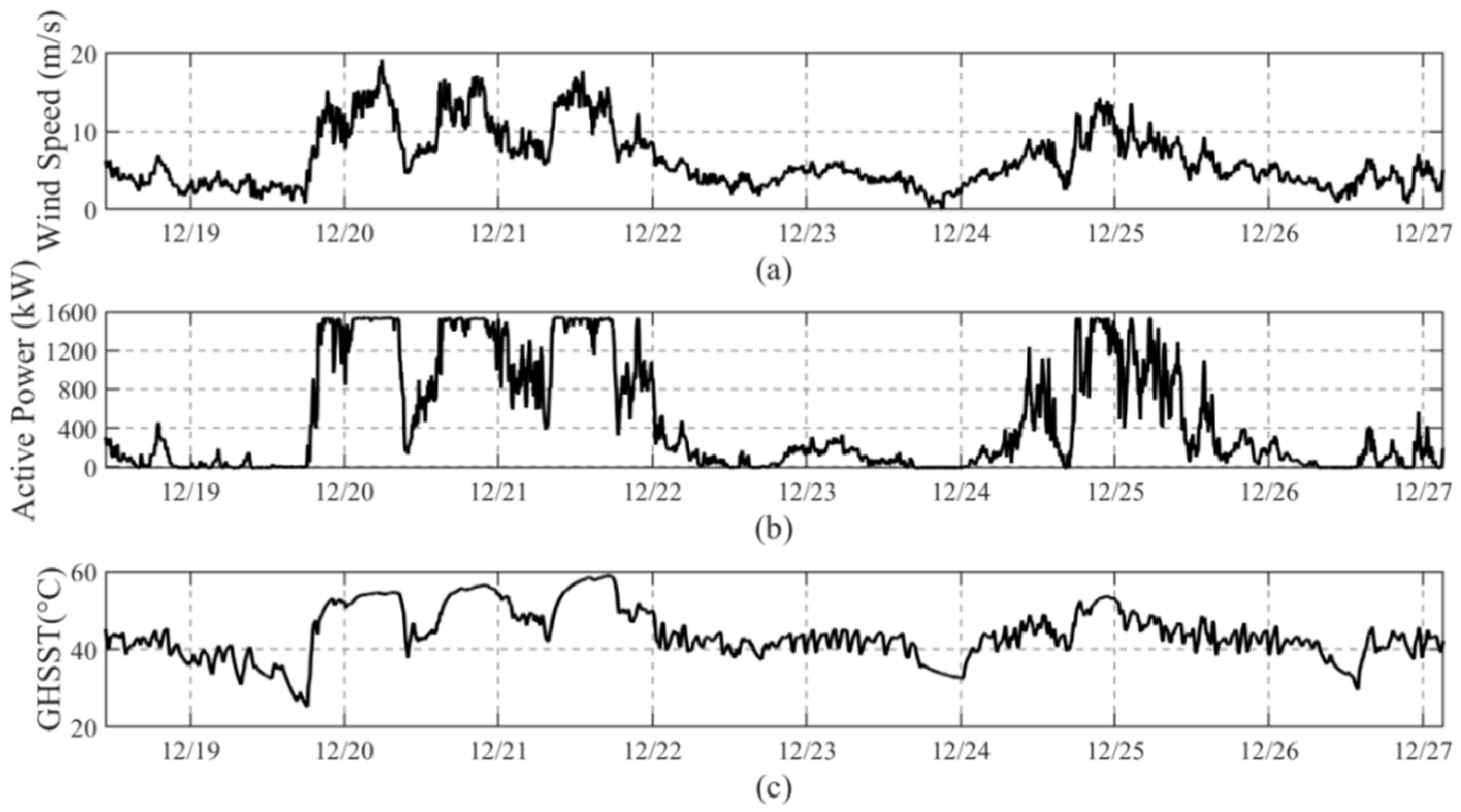
Traditional fault detection methods using SCADA data focus on the secondary effects of faults, with abnormal conditions often detected through heat generation in gearbox components. While the SCADA system monitors hundreds of different signals, this study concentrates on high-temperature fault-related signals to construct the normal behavior model. A subset of the monitored data is presented in Figure 5. The figure depicts the time histories of wind speed, active power, and GHSST from 18 December to 25 December. These variables exhibit similar trends; however, the active power responds almost instantaneously to changes in the wind speed, while GHSST demonstrates a delayed response to active power. Specifically, wind speed varies between 0 m/s and 20 m/s, exceeding the rated wind speed of 11 m/s during four distinct periods. During these intervals, the power output reached its rated power of 1500 kW. Conversely, when wind speed was below the cut-in speed of 3 m/s, the turbine generated no power. When the turbine operated at low power, the GHSST fluctuated around 40 °C. During turbine shutdown, the GHSST gradually decreased, occasionally falling below 30 °C, depending primarily on the ambient temperature. When the turbine resumed operation at rated power, the GHSST rapidly increased, reaching 50 °C, after which the temperature rise rate slowed and gradually stabilized within the range of 55 °C to 60 °C. The correlation among these variables supports the feasibility of diagnosing and predicting turbine performance based on SCADA monitoring signals.

In this study, the operational data from two wind turbines, WT#106 and WT#122, within the wind farm were selected as the primary dataset due to their diverse anomalies and GHSS fault occurrences. The dataset covers a period from 00:00:00 on 1 December 2022, to 07:00:00 on 15 February 2023. Data were sampled with high frequency but recorded at five-minute intervals, yielding a total of 21,876 data points. After applying a comprehensive data cleaning process to WT#106, 18,940 data points were retained, indicating that approximately 13.4% of the recorded data were identified as noise and subsequently removed. For WT#122, a total of 18,695 data points remained post-cleaning, with about 14.5% deemed noise and extracted

3.2. Data Cleaning Algorithm and Verification

3.2.1. Anomalous Data Identification

Anomalous data can be effectively cleaned based on their spatial distribution characteristics on the WSP curve, ensuring a robust approach applicable to various types of anomalies. The anomalous data can be categorized into four types, based on the operational status and distribution characteristics, as illustrated in Figure 6.

• Shutdown point: The turbine is shut down due to faults, sensor failures, or scheduled maintenance, leading to zero power output irrespective of wind speed. In the WSP graph, the output power remains at 0 even when the wind speed exceeds the cut-in threshold.
• Discrete outliers: These abnormal data points exhibit irregular dispersion, typically arising from random events such as sensor malfunctions or sudden climatic changes. In the WSP graph, they appear as irregularly scattered data points.

• Power curtailment: These data points primarily stem from the curtailment of wind power. Although the turbines function normally, factors such as grid constraints, instability in wind power generation, or mismatched construction schedules prevent full power operation. The characteristic feature of such data is a constant active power, represented as a horizontal straight line in the graph. This phenomenon does not occur in all turbines.
• Wind measurement anomalies: These anomalies occur due to anemometer measurement errors, resulting in a shape similar to the probability power curve. They appear either above or below the expected probability power curve.

3.2.2. Anomalous Data Cleaning

Shutdown point: When the wind speed is between the cut-in and cut-out wind speeds, the generator operates and the output power is non-zero. Therefore, the SCADA data should be truncated according to Equation (8).

$$\left\{P_i\le 0\right\}\cap \left\{V_{in}<V_i<V_{out}\right\}.$$

(8)

In this equation, P_i represents the output power at time i, V_i is the corresponding wind speed, and V_in and V_out denote the cut-in and cut-out wind speeds, respectively.

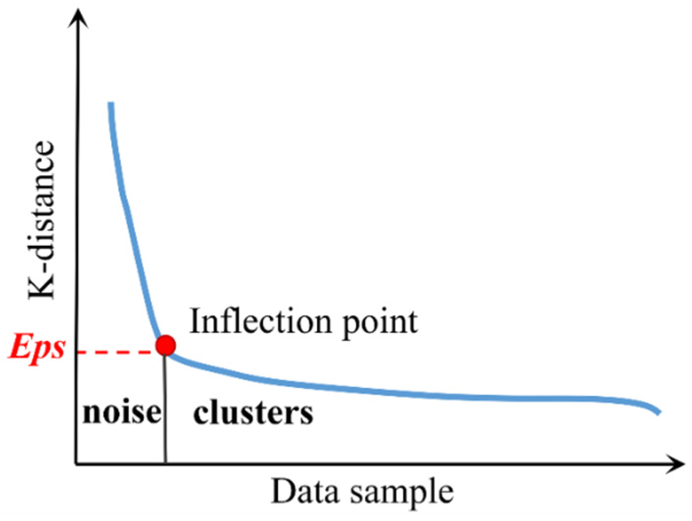
The key characteristic of discrete noise data is its random and scattered distribution, making it difficult to describe using a mathematical model. We adopt DBSCAN for identifying the discrete points [41]. The DBSCAN method has two parameters to be determined, the domain radius Eps and the minimum number of points within the domain radius MinPts. K-distance curves are drawn, and the value at the inflection point is set as the domain radius Eps, as shown in Figure 7, where the K-distance is the distance between each data point and the k-th nearest point.

The substantial volume of the SCADA data from wind turbines in this study necessitated an optimized parameter selection methodology. We developed an adaptive sample-size-based approach, where the key parameter k is determined by the heuristic relationship k = ln(N_total), with N_total denoting the total number of data. The conventional determination of MinPts typically relies on the mathematical expectation of sample counts within Eps-neighborhoods. However, the SCADA data from wind turbines presents two critical challenges: (1) massive normal dataset scales and (2) high-density distributions within Eps-neighborhoods. The direct application of statistical expectations would yield excessively large MinPts values, thereby compromising clustering efficacy. Given that the DBSCAN clustering objective focuses on detecting sparsely distributed anomalies that deviate from normal operational clusters, which typically constitute approximately 10% of the dataset, this work proposes the following empirically validated formula to determine MinPts:

$$N_{noise}=N_{total}\times 10\%,$$

(9)

$$MinPts={\displaystyle \frac{1}{N_{noise}}}{\displaystyle \sum }_{i=1}^{N_{noise}}{N}_{Eps-nbhd}^i,$$

(10)

where $N_{Eps-nbhd}^i$ represents the amount of data within the i-th Eps-neighborhood, and these values are arranged in ascending order. A smaller number of data points within the neighborhood indicates a more discrete data distribution, suggesting a higher likelihood of the presence of discrete abnormal points. In this paper, the values of $N_{Eps-nbhd}^i$ are sorted in ascending order, which shows that the earlier a neighborhood is in the sequence, the fewer data points it contains, while the data points become denser as the sequence progresses. By calculating the mean value of the top 10% of $N_{Eps-nbhd}^i$ values, a more suitable MinPts value can be identified among discrete abnormal points more effectively.

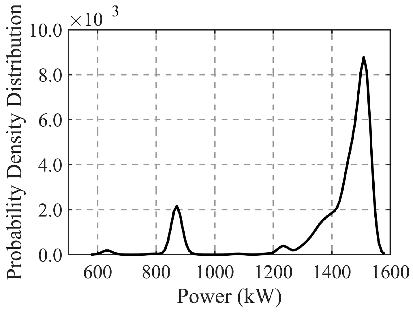
KDE is a non-parametric method employed to estimate the probability density function (PDF). KDE applies a smooth kernel function to fit the observed data points, thereby approximating the underlying probability distribution. The presence of stacked anomalous data can result in bimodal or multimodal distributions in the PDF. To address this issue, the PDF curves of power scatter points across various wind speed intervals are adjusted by peak-shaving to eliminate anomalies associated with low-density peaks. This process transforms multimodal distributions into unimodal ones, effectively cleaning the stacked power limitation data.

Take WT#106 with a wind speed range of 10–13 m/s as an example, as shown in Figure 8. Under normal operating conditions, the active power should be approximately 1500 kW. However, due to the presence of a power limitation, the power in this wind speed range occasionally drops to around 870 kW. The peak-shaving process can remove outputs below 1000 kW in this interval. The figure also shows small peaks at 630 kW and 1230 kW, indicating power-limiting points that require cleaning.

The distribution of these anomalies in the WSP scatter plot resembles the main shape under normal operation. A sigmoid curve is applied to fit the wind speed–power scatter plot, and points beyond the quartile distance from the fitted curve are removed to complete the cleaning of the anemometer noise data. The mathematical expression of the sigmoid curve is shown in Equation (11).

$$f\left(x\right)={\displaystyle \frac{a}{b+e^{-\left(d·x-v\right)}}}.$$

(11)

Since the number of noisy data points is small and appears randomly, direct deletion has minimal impact on the overall data distribution. Therefore, deleting the entire timestamp containing noise points preserves the spatiotemporal relationships of each variable and ensures high-quality data for subsequent analyses.

3.2.3. Data Cleaning Case

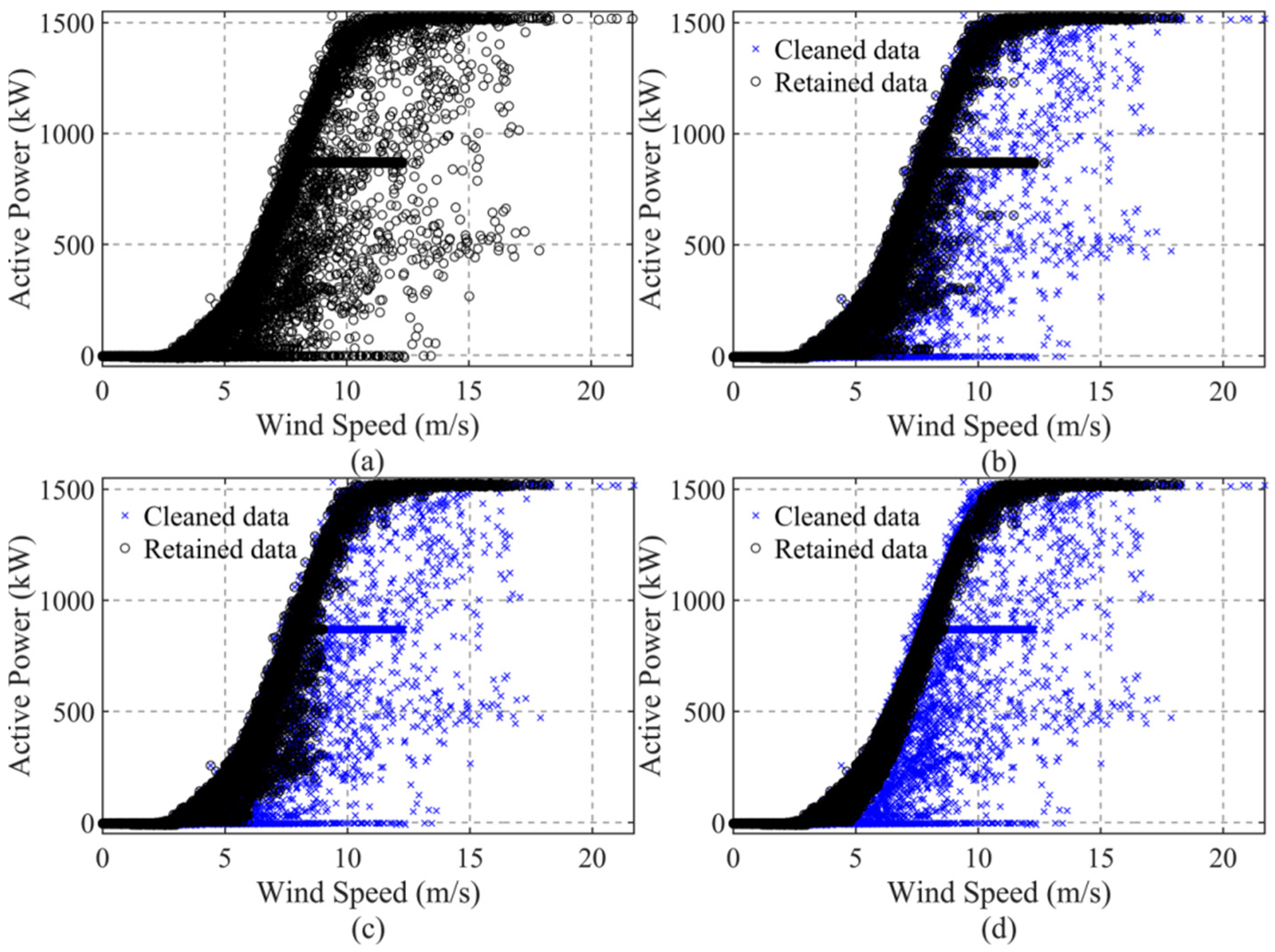
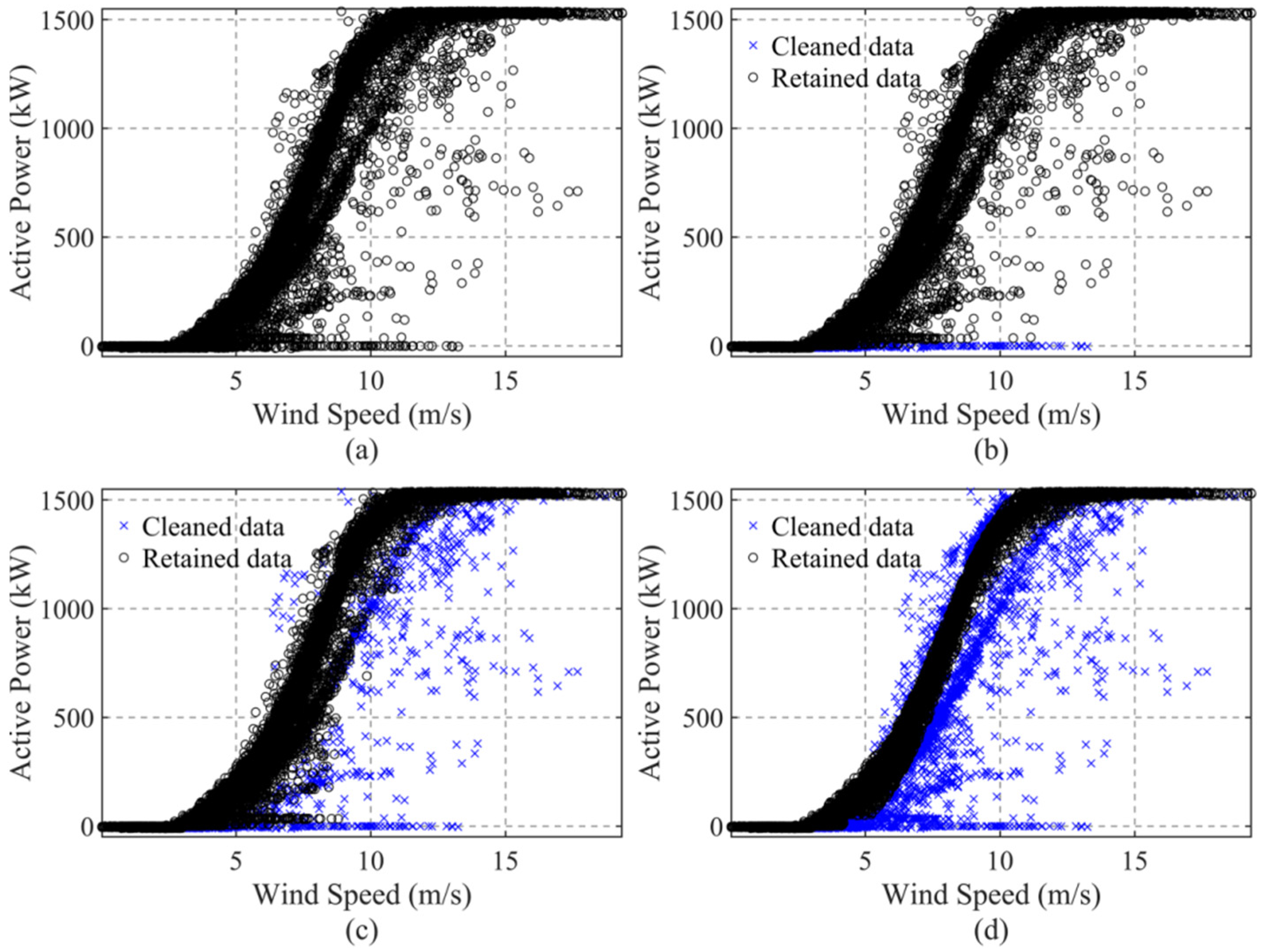
Before data cleaning, it is essential that we analyze the distribution characteristics of the original WSP curve to identify the types of anomalies. The cleaning process should then be customized according to each specific anomaly type. To comprehensively demonstrate the effectiveness of the proposed data cleaning algorithm, the operational monitoring data from WT#106, which contains all types of noise data, was selected for cleaning. According to the original power curve as shown in Figure 9a, the data contains shutdown points, discrete noise points, power curtailment points, and stacked anomalies below the normal power curve. The stacked noise points below the curve exhibit an upward trend similar to that of the original curve, indicating wind measurement anomalies. The results of the targeted and step-by-step cleaning process, as described in Section 2.2, are shown in Figure 9b–d.

First, the truncation method and DBSCAN clustering are applied to clean the downtime points and discrete noise points. The results are shown in Figure 9b. At this stage, the power-limited points become more intuitively visible, and the probability density characteristics are more apparent. In Figure 9c, KDE is used to clean the power-limiting points. The lower part of the curve contains stacked noise points with a trend similar to that of the main body of the normal data points. The fitting method is then employed to remove points that deviate more than the 95th percentile from the fitted curve. Figure 9d displays the final cleaning results, where noise data is thoroughly removed while maximizing the retention of normal operational data.

The wind measurement anomalies in WT#122 are more pronounced. An examination of the original power scatters in Figure 10a reveals stacked shutdown points, discretely distributed anomalous data, and side wind anomalies with a trend similar to the normal wind speed–power curve. First, the truncation method is applied to remove downtime data points, with the results shown in Figure 10b. DBSCAN clustering is then used to eliminate discrete noise points, as shown in Figure 10c. The characteristics of wind measurement anomalies are clearly visible, along with power-limiting points at the bottom of the curve. These anomalies are cleaned using the fitting method, with the final results displayed in Figure 10d.

3.3. Data Normalization

In deep learning models, normalization ensures that the value ranges of different features are comparable, preventing certain features from disproportionately influencing the loss function during training. This accelerates model convergence, improves training efficiency, and mitigates issues such as gradient explosion and vanishing gradients. Furthermore, normalization enhances the model’s performance and generalization ability, ensuring stability and robustness when handling features with different units and scales. Therefore, normalization is a crucial step in ensuring an efficient and robust model operation.

For preprocessing SCADA monitoring variables, this study employs z-score normalization to standardize features with different scales into a standard normal distribution (mean of 0, and standard deviation of 1). This process eliminates disparities in feature scales and ensures that each feature contributes equally during model training. The z-score is calculated according to Equation (12):

$$Z={\displaystyle \frac{I-mu}{sig}},$$

(12)

where Z represents the normalized matrix, I denotes the input matrix, mu is the vector of the means of each variable, and sig is the vector of the standard deviations of each variable.

3.4. Feature Selection

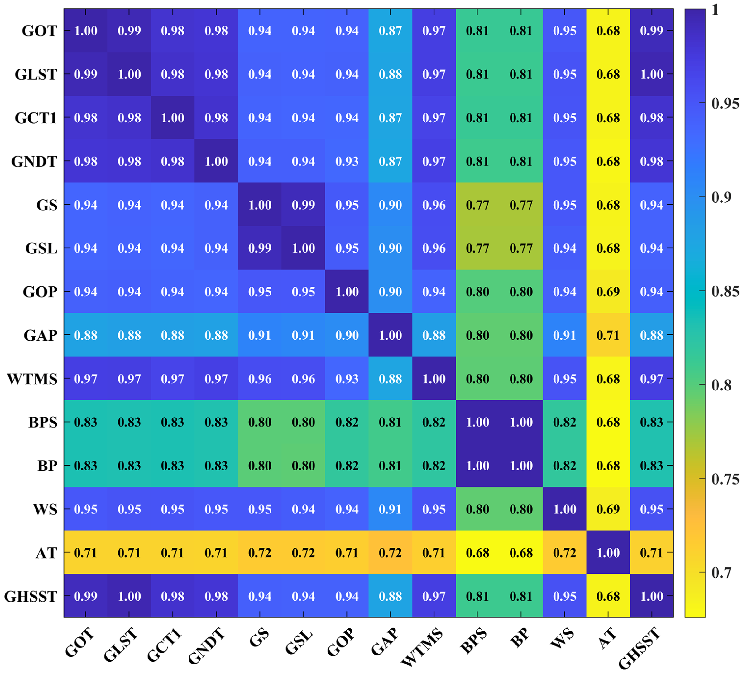
The SCADA system is a comprehensive data monitoring and acquisition platform that tracks dozens, or even hundreds, of parameter variables. Directly using all these variables for data modeling may introduce redundant information. Therefore, it is essential that we select the most relevant variables. The GHSST is chosen as the model’s target variable. The grey relational analysis (GRA) method is employed to identify the key factors influencing this temperature. GRA assesses the strength of relationships between the target temperature and other operational state variables, even in cases of incomplete data. By quantifying the similarity between data series, GRA identifies variables with higher grey correlation coefficients, which are then selected as input features for the training model.

The grey relational degree is calculated as shown in Equation (13):

$${\zeta }_i\left(l\right)={\displaystyle \frac{\underset{i}{\min }\underset{l}{\min }\left|x_0\left(l\right)-x_i\left(l\right)\right|+\rho \cdot \underset{i}{\max }\underset{l}{\max }\left|x_0\left(l\right)-x_i\left(l\right)\right|}{\left|x_0\left(l\right)-x_i\left(l\right)\right|+\rho \cdot \underset{i}{\max }\underset{l}{\max }\left|x_0\left(l\right)-x_i\left(l\right)\right|}}$$

(13)

where x₀ represents the temperature of the high-speed shaft of the gearbox (the parent sequence), x_i denotes other variables monitored by the SCADA system (the subsequences), i represents different monitored variables, l is the length of the monitoring sequence over the selected time period, and ρ is the resolution coefficient, set to 0.5 in this study, balancing outlier suppression and relational discrimination for SCADA data. Once the correlation coefficient matrix is derived from this equation, the correlation coefficients for each variable are averaged. This average quantifies the grey correlation between any SCADA-monitored variable and the GHSS temperature.

SCADA-monitored parameters can be divided into two categories based on their correlation with wind speed. The first category includes parameters significantly affected by wind speed, such as the component temperature, generator speed, and power. The second category comprises parameters primarily influenced by environmental factors and factory performance, such as the yaw position and lubricating oil pressure. Since wind turbine faults are typically caused by environmental factors in the absence of performance degradation, this study focuses on the first category of parameters. The model extracts features strongly correlated with abnormal operating states for in-depth fault diagnosis.

Taking the data of WT#106 as an example, the GHSST is designated as the target variable for feature selection. Fourteen variables were used for the GRA calculation, with the data input into Equation (13). The computational results, as illustrated in Figure 11, demonstrate that the majority of variables maintain high grey relational coefficients with the target parameter. Only three variables—blade pitch setpoint, BPS, blade position, BP, and ambient temperature, AT—exhibited relatively weaker correlations. Based on the GRA outcomes, the top ten variables with the highest grey relational coefficients were selected as candidate inputs for the multi-source input prediction model. Note that the generator speed limit (GSL) exhibits a high correlation coefficient with the target variable. However, it was excluded as an input due to its inherent operational constraints. Specifically, the GSL is confined within a predefined safe range during normal operation. When the GSL approaches either its upper or lower boundary limits, it loses its capability to effectively reflect the variations in the GHSST. This limitation in dynamic responsiveness makes the GSL unsuitable as a predictive input parameter for the model. Therefore, the final selection of input features for multivariate prediction consists of nine variables, as shown in

Table 1. Selected input features for multivariate prediction.

No	Variable	Abbreviations	Location
1	Gearbox low-speed shaft temperature	GLST	Gearbox
2	Gear oil temperature	GOT	Gearbox
3	Generator coil 1 temperature	GCT1	Generator
4	Generator non-driven end temperature	GNDT	Generator
5	Main state of the wind turbine	WTMS	Synthesis
6	Wind speed	WS	Environment
7	Gearbox speed	GS	Gearbox
8	Gear oil pressure	GOP	Gearbox
9	Grid active power	GAP	Grid

.

4. STA-BKA Principle

4.1. Spatial Feature Extraction

The multivariate spatial correlations within SCADA data streams are systematically modeled through a multi-tier convolutional topology [42], as illustrated in Figure 12. The technical implementation involves two cascaded convolutional layers with kernel dimensions k = {3,5}, which operate as follows:

$$X_k^{\left(m\right)}=ReLU\left({\displaystyle \sum }_{c=1}^C{W}_k^{\left(c,m\right)}\ast X_{k-1}^{\left(c\right)}+b_j^{\left(m\right)}\right),$$

(14)

where $X_k^{\left(m\right)}$ represents the output feature map of the m-th convolutional kernel in the k-th layer, $W_k^{\left(c,m\right)}$ denotes the weight matrix, * is the convolution operator, $X_{k-1}^{\left(c\right)}$ refers to the local input feature of the c-th convolution operation in the k-th layer, and $b_j^{\left(m\right)}$ is the bias.

The pooling layer is employed to reduce the amount of data and parameters, thereby enhancing the feature invariance of the data. The mathematical formulation of the pooling layer is given by the following:

$$P_k^{\left(i,j\right)}=\underset{\left(j-1\right)w+1<\tau <jw}{max}\left\{q_k^{\left(i,\tau \right)}\right\},j=1,2,\cdots ,m,$$

(15)

where $P_k^{\left(i,j\right)}$ represents the j-th pooling value of the i-th output map in the k-th layer, $q_k^{\left(i,\tau \right)}$ denotes the local input feature of the j-th pooling operation in the k-th layer, and w is the width of the pooling region.

Crucially, the hierarchical feature abstraction mechanism suppresses redundancy via nonlinear activation and pooling operations, maintains temporal coherence by preserving raw data sequences’ chronological integrity, and enables operational adaptability through translation-invariant cross-variable mappings. Furthermore, the dropout technique randomly deactivates neurons during training [43] to mitigate overfitting. This reduces the network’s complexity and neuron interdependency, improving the model’s generalization performance. This architecture guarantees a seamless compatibility with subsequent LSTM-based temporal modeling, particularly for handling wind turbine operational regime transitions.

Figure 12 illustrates a hierarchical feature extraction architecture designed for processing SCADA monitoring variables. The input tensor $X_{SCADA}\in R^{N_{in}\times T}$ represents N_in variables over T time steps, with variable abbreviations defined in Table 1. After convolution and activation by Kernel #1, feature maps are generated with an additional channel. Then, through the pooling layer, the dimension of the variables is reduced to N′. The calculation process of the second convolutional layer is similar to that of the first one. The variable dimension is further reduced to N″, and the number of channels becomes N_channel2. The final output is named H_Conv. Critically, the temporal dimension T remains invariant throughout the hierarchical transformations, ensuring the integrity of the sequential patterns.

4.2. Temporal Feature Extraction

LSTM networks represent a specialized variant of RNNs that excel in processing and predicting sequential data [44,45]. Unlike standard RNNs, which often struggle with long-term dependencies due to vanishing and exploding gradient problems, LSTM networks incorporate an innovative gating mechanism that effectively addresses these limitations [46]. This architectural advancement enables the more stable and accurate processing of extended temporal sequences. The detailed structural configuration of LSTM units is presented in Figure 13.

The hierarchical convolutional output H_Conv undergoes tensor reshaping to serve as the input for the LSTM temporal modeling module, and the temporal dimension T is preserved through a dimension transformation operation. The input dimension D = N″ × N_channel2 for each time step, all channels are expanded to one dimension, and the input X_lstm of LSTM layer can be expressed as $X_{\mathrm{lstm}}=\left[X_{lstm}^1,X_{lstm}^2,...,X_{lstm}^T\right]$, and the output is H_lstm1 after the first layer of the LSTM network, whose output dimension is T × h₁, where h₁ is the number of hidden units in the first layer. After the two layers of LSTM for temporal modeling, the output is H_lstm2.

The LSTM unit is composed of three components, the forget gate f_t, the input gate i_t, and the output gate o_t, which are responsible for controlling the memorization, updating, and output of information, respectively. The specific computational steps are outlined as follows:

$$f_t=\mathrm{sig}\left(W_f\left[h_{t-1},x_{lstm}^t\right]+b_f\right),$$

(16)

$$i_t=\mathrm{sig}\left(W_i\left[h_{t-1},x_{lstm}^t\right]+b_i\right),$$

(17)

$$c_t=f_t{c}_{t-1}+i_c\tanh \left(W_c\left[h_{t-1},x_{lstm}^t\right]+b_c\right),$$

(18)

$$o_t=\mathrm{sig}\left(W_o\left[h_{t-1},x_{lstm}^t\right]+b_o\right),$$

(19)

$$h_t=o_t\tanh \left(c_t\right),$$

(20)

where sig(•) represents the Sigmoid activation function, and W_f, W_i, W_c, and W_o are the weight matrices corresponding to the forget gate, input gate, cell state, and output gate, respectively. Similarly, b_f, b_i, b_c, and b_o denote the bias terms for these gates. h_t−1 represents the hidden state from the previous time step, $x_{lstm}^t$ is the current input, c_t is the current cell state, and h_t is the final output determined by both the output gate and the cell state. These gating mechanisms allow LSTM to selectively retain and update information in long time series, thereby enhancing its predictive capability in time-dependent tasks. The LSTM layers transform the local features extracted by the convolutional layers into more time-aware higher-order features, capable of handling long-term dependencies in device operation and complex time-series patterns.

4.3. Global Information Capture

Self-attention has emerged as a fundamental component in deep learning, particularly for sequence modeling tasks. By computing correlation weights between sequence elements and dynamically adjusting feature importance, SA effectively captures long-range dependencies and enables precise information extraction [47].

The SA mechanism is introduced into the GHSS temperature prediction framework to enhance temporal dependency modeling and address the inherent limitations of LSTM networks in capturing long-range dependencies. The integration of SA with LSTM provides key advantages for GHSS monitoring: SA reduces the LSTM’s sequential computation complexity from O(T²) to O(TlogT) through parallelizable attention operations, and the direct attention pathways alleviate gradient vanishing issues in deep LSTM networks. The combined architecture leverages LSTM’s localized temporal dynamics and SA’s global context awareness, resulting in a hierarchical feature representation optimized for temperature prediction. Through a global attention mechanism, SA dynamically assigns temporal attention weights to historical states, thereby emphasizing critical operational patterns in wind turbine SCADA data. To further optimize the attention process, a multi-head attention architecture is implemented, which operates through parallel attention heads.

In the proposed prediction framework, the SA module processes the hidden states H_lstm2 generated by the preceding LSTM layer. Through learnable parameter matrices W^Q, W^K, and W^V, the input states are projected into the query (Q), key (K), and value (V) vectors to compute the attention weights. As illustrated in Figure 14, this transformation is mathematically formulated as follows:

$$Q=H_{lstm}{W}^Q,\hspace{1em}K=H_{lstm}{W}^K,\hspace{1em}V=H_{lstm}{W}^V,$$

(21)

$$hea{d}_i=\mathrm{softmax}\left({\displaystyle \frac{Q_i{K}_i^T}{\sqrt{d_k}}}\right)V,i=1,\dots ,nu{m}_h,$$

(22)

$$H_{sa}=\mathrm{concat}\left(hea{d}_1,\dots ,hea{d}_{16}\right)W_H,$$

(23)

where d_k is the dimension of the key vector, and the softmax function is applied to transform the dot product results into a weight distribution. num_h denotes the number of attention heads, which is set to 16. The 16 attention heads optimize feature diversity across temporal subspaces while maintaining computational efficiency, and each head independently learns distinct temporal-scale features (e.g., minute-level local change or hour-level degradation trends), effectively mitigating information loss through diversified feature subspace projections. W_H is the weight matrix for further linear transformation after splicing the outputs of the 16 heads. The integration of the self-attention mechanism significantly improves the model’s feature representation power, particularly for capturing progressive failure precursors.

4.4. BKA Optimization

BKA is a nature-inspired meta-heuristic optimization framework that emulates the migratory and predatory behaviors of black-winged kites [48]. This algorithm integrates two complementary strategies: (1) the Cauchy mutation operator, which facilitates the escape from local optima and enhances global search capabilities, and (2) the leader-based guidance mechanism, which utilizes the current best solution to direct the search trajectory. The synergistic combination of these strategies achieves an optimal balance between global exploration and local exploitation, rendering BKA particularly effective for high-dimensional, complex optimization problems.

The BKA implementation follows a systematic procedure. Initialization begins with generating a population of random solutions within the search space. Subsequently, the algorithm simulates various predatory attack behaviors to conduct the global exploration. The mathematical formulation of these attack behaviors is expressed as follows:

$$y_{t+1}^{i,j}=\left\{\begin{array}{cc}{y}_t^{i,j}+\lambda \left(1+\sin (\eta \right))\times y_t^{i,j}& p<\eta \\ y_t^{i,j}+\lambda \times \left(2\eta -1\right)\times y_t^{i,j}& \mathrm{else}\end{array}\right.,$$

(24)

$$\lambda =0.05\times e^{-2\times {\left({\displaystyle \frac{t}{T}}\right)}^2}.$$

(25)

$y_t^{i,j}$ and $y_{t+1}^{i,j}$ denote the positions of the i-th kite in the j-th dimension at iteration t and t+1. η is a random value between 0 and 1. The parameter p controls the switching between attack behaviors and significantly affects the algorithm’s accuracy and stability. Its optimal value (p = 0.9) is determined empirically, achieving the best or competitive results in most scenarios [48]. T is the total number of iterations, and t represents the current iteration count.

The migration process in BKA follows a dynamic leadership mechanism. When the fitness value of the current population falls below that of a randomly selected population, the incumbent leader abdicates its position and integrates into the migrating group, indicating sub-optimal leadership performance. Conversely, if the current population demonstrates superior fitness compared to the random population, the leader maintains its guiding role, steering the group toward potential optimal solutions. The migration behavior of the black-winged kite is mathematically expressed as follows:

$$y_{t+1}^{i,j}=\left\{\begin{array}{cc}{y}_t^{i,j}+C\left(0,1\right)\times \left(y_t^{i,j}-L_t^j\right)& F_i<F_{ri}\\ y_t^{i,j}+C\left(0,1\right)\times \left(L_t^j-\theta \times y_t^{i,j}\right)& else\end{array}\right.,$$

(26)

$$\theta =2\times \sin (\eta +\pi /2).$$

(27)

$L_t^j$ represents the leader of the j-th dimensional kite at iteration t. $y_t^{i,j}$ and $y_{t+1}^{i,j}$ denote the positions of the i-th kite at iteration steps t and t+1 in the j-th dimension, respectively. F_i indicates the i-th dimensional current position of any kite in iteration t, while F_ri is the fitness value of a random kite in the i-th dimension at iteration t. C(0, 1) represents the Cauchy mutation [49]. The one-dimensional Cauchy distribution is a continuous probability distribution characterized by two parameters, and its probability density function is as follows:

$$f\left(x,{\delta }_c,{\mu }_c\right)={\displaystyle \frac{1}{\pi }}{\displaystyle \frac{{\delta }_c}{{\delta }_c^2+{(x-{\mu }_c)}^2}},\hspace{1em}-\infty <x<\infty ,$$

(28)

$$f\left(x,{\delta }_c,{\mu }_c\right)={\displaystyle \frac{1}{\pi }}{\displaystyle \frac{1}{x^2+1}},\hspace{1em}-\infty <x<\infty .$$

(29)

When δ_c = 1 and μ_c = 0, the probability density function takes the standard form.

5. Results

5.1. NCM Based on GHSST

5.1.1. STA-BKA Model Parameters

Following the feature variable selection procedure outlined in Section 3.4, nine variables were selected as input features to capture the key aspects of the system’s operational dynamics. Based on these inputs, a deep learning network model was developed to perform a multivariate prediction of the GHSST. After data cleaning, 18,940 SCADA data points were retained for WT#106 and 18,695 for WT#122. The dataset was divided into training and testing subsets, with 80% of the data allocated for training and the remaining 20% set aside for testing, thus ensuring a rigorous evaluation of the model’s performance.

To construct the spatio-temporal hybrid model incorporating a self-attention mechanism, two convolution layers were employed to effectively extract the spatial local features. These were followed by two LSTM layers to capture the temporal dependencies of the sequential data. The self-attention mechanism was introduced to enhance the model’s ability to represent global dependencies, thereby improving the robustness of the temporal information available for predictions. Within the current study, the rectified linear unit activation function was implemented to introduce nonlinearity, facilitating the model to learn complex patterns. Furthermore, L2 regularization was applied as a strategy to mitigate overfitting, subsequently followed by a regression analysis to predict the GHSST.

The architecture employs two convolutional layers with 32 filters and 64 filters, respectively, for spatial feature extraction, connected to two LSTM layers containing 128 and 64 units to capture temporal dependencies. A dropout layer (rate = 0.2) is inserted after the LSTM layer to mitigate overfitting, while a 16-head self-attention mechanism (key dimension = 64) adaptively weights critical features. This hierarchical design systematically integrates spatial modeling, sequential pattern learning, and feature prioritization.

During the training process, the network’s hyperparameters were optimized utilizing the BKA technique. The Adam optimization algorithm was selected for its adaptive learning rate capabilities, which improve the convergence efficiency [50]. To prevent potential gradient explosions, a threshold of 1 was imposed. Furthermore, an early stopping strategy was implemented to enhance the model’s generalization and to conserve computational resources and time.

Notably, the learning rate, batch size, and regularization coefficient of the STA hybrid model were optimized through the BKA. The learning rate, a crucial hyperparameter, determines the step size taken at each iteration while approaching the minimum of the loss function. A well-optimized learning rate can significantly accelerate convergence and maintain training stability, allowing the model to learn effectively without overshooting the optimal solution. The batch size, indicating the number of training samples processed per iteration, was also carefully considered. Although larger batch sizes can speed up training, they may compromise generalization performance. Conversely, smaller batch sizes can improve generalization but often at the cost of longer training times. The regularization coefficient is essential for controlling overfitting by penalizing overly complex models, ensuring that the model maintains generalizability to unseen data.

To quantitatively evaluate the model’s performance, the root mean square error (RMSE) was adopted as the fitness function, as defined in Equation (32). The RMSE provides a straightforward yet effective measure of the discrepancy between the predicted and observed values, accurately reflecting the model’s predictive capability. It is particularly suitable for this task as it imposes a heavier penalty on larger prediction errors, which is critical when predicting time-sensitive parameters such as the GHSST. The minimum RMSE was attained through BKA, enabling the determination of optimal parameters. The accuracy of the STA hybrid model profoundly influences the overall quality of the prediction. The specific BKA settings are presented in

Table 2. Parameter settings of the BKA optimization.

Parameter Setting	Parameter Values
Population size pop	5
Maximum number of iterations Iter	10
Parameter lower limit lb	[0.0001, 10, 0.00001]
Parameter upper limit ub	[0.01, 300, 0.01]

, which further elucidates the computational parameters. The population size, pop, and the number of iterations, Iter, are two critical parameters for the algorithm. Note that these two parameters are quite small, corresponding to the problem scale. Given the prediction task only involves 10 input variables and 1 output, and only 3 hyperparameters requiring optimization in the STA model, the small pop and Iter would efficiently explore the solution space while aligning with deep learning hyperparameter tuning conventions. Figure 15 demonstrates convergence within 10 generations. The convergence curve of WT#122 exhibits smoother fitness reduction, while that of WT#106 shows accelerated initial convergence. Both achieve stabilization within 10 iterations, validating the parameter configuration (pop = 5, Iter = 10), where minor fluctuations reflect stochastic exploration during migration phases.

Figure 15 illustrates the optimization process of the BKA by plotting the variation in best fitness values over ten iterations. In Figure 15a, the best fitness value decreases from approximately 0.924 to about 0.884, indicating effective convergence toward an optimal solution. The stable fluctuations highlight the robustness of the algorithm in complex optimization tasks. On the other hand, Figure 15b exhibits a fitness range declining from 1.396 to 1.362, demonstrating swift convergence and reinforcing the efficiency of the BKA in achieving lower fitness values. After hyperparameter optimization, the learning rate, batch size, and regularization coefficient were determined as 0.0017, 256, and 0.00045, respectively, based on model characteristics. Collectively, these results demonstrate the ability of BKA to improve prediction accuracy in practical applications of optimizing wind turbine performance.

5.1.2. Analysis of Results

The hybrid deep learning model described above was employed to predict the GHSST ten minutes into the future. To validate the accuracy of the proposed STA-BKA prediction model, its performance was compared with that of the CNN-LSTM and LSTM models. The network architectures and layers in both the CNN-LSTM and LSTM models were consistent with those utilized in the proposed hybrid model.

To evaluate the prediction errors on the validation set, this study employed four metrics: the mean absolute error (MAE), the mean absolute percentage error (MAPE), the RMSE, and the coefficient of determination (R²). Their respective calculation formulae are provided as follows:

$$\mathrm{MAE}={\displaystyle \frac{1}{N}}{\displaystyle \sum }_{j=1}^N\left|{\widehat{y}}_j-y_j\right|,$$

(30)

$$\mathrm{MAPE}={\displaystyle \frac{1}{N}}{\displaystyle \sum }_{j=1}^N\left|{\displaystyle \frac{{\widehat{y}}_j-y_j}{y_j}}\right|,$$

(31)

$$\mathrm{RMSE} =\sqrt{{\displaystyle \frac{1}{N}}{\displaystyle \sum }_{j=1}^N{\left(y_j-{\widehat{y}}_j\right)}^2},$$

(32)

$${\mathrm{R}}^2=1-{\displaystyle \frac{{{\displaystyle \sum }}_j{\left({\widehat{y}}_j-y_j\right)}^2}{{{\displaystyle \sum }}_j{\left({\overline{y}}_j-y_j\right)}^2}},$$

(33)

where ŷ_j denotes the predicted value, y_j is the measured value, N is the number of samples, and j ranges from 1 to N, indicating the j-th sample. Lower MAE, MAPE, and RMSE values indicate a smaller prediction error and higher accuracy. Meanwhile, R² approaches 1 as the model’s fit improves, indicating a stronger agreement between the predicted and observed values.

Figure 16 presents a detailed comparison of the predictive performance of multiple models for the GHSST of WT#106. The dataset illustrated in the figure encompasses the actual temperature values alongside the predicted outcomes generated by three distinct algorithms: LSTM, CNN-LSTM, and the STA-BKA model proposed in this study. Notably, the red dotted line corresponding to the STA-BKA model aligns closely with the actual data points, signifying the model’s superior predictive performance throughout the comprehensive evaluation dataset.

The hybrid model provides superior accuracy across all observed temperature states. The model effectively captures complex patterns in the temperature data, producing predictions that closely correlate with the actual temperature readings. It is worth noting that the model occasionally underestimates the peak temperatures. Although the algorithm occasionally suffers from minor discrepancies, particularly in transitional regions of rapidly changing temperatures, the algorithm performed well in the vast majority of cases, effectively maintaining a low prediction error margin.

The CNN-LSTM model’s prediction results are equally commendable, ranking in the middle in performance. It adequately captures the overall temperature trend but lacks the BKA algorithm’s accuracy. As Figure 16a shows, CNN-LSTM performs well in lower-temperature states but fails to accurately predict the peaks in higher-temperature states, where discrepancies with the actual data are large, as shown in Figure 16b. In smooth fluctuation states, the model tracks the general trend but lacks the attention mechanism’s ability to automatically focus on key information and process long sequences efficiently. Consequently, it exhibits more oscillations than STA-BKA, as illustrated in Figure 16c.

The standard LSTM model yields the least favorable results among the evaluated models. While it captures the general trend of the temperature variations, it suffers from significant underfitting, especially noticeable in both the higher temperature state and during periods of rapid fluctuation. The LSTM struggles to adapt to the dynamic temperature changes, leading to a noticeable lag and higher prediction errors. In the lower temperature state, although the model somewhat follows the trend, it lacks the robustness and accuracy exhibited by the other models, particularly in capturing subtle fluctuations.

A comparative analysis shows the advantages of integrating optimization techniques with deep learning architectures. The STA-BKA model demonstrates enhanced predictive capabilities and highlights how attention mechanisms capture temporal dependencies in complex datasets. The results confirm that our proposed model significantly outperforms traditional methodologies and demonstrates the potential for accurate temperature forecasting in real-world applications. This analysis highlights the need for advanced hybrid approaches when handling time-series prediction complexities.

Table 3. Calculation results of evaluation indices of different models of WT#106.

	MAE/°C	MAPE/%	RMSE/°C	R2
LSTM	1.7015	4.4087	2.1986	0.9181
CNN-LSTM	1.2504	3.3665	1.5917	0.9571
STA-BKA	1.0233	2.7039	1.3886	0.9673

provides quantitative metrics for each model. The STA-BKA model achieves the lowest values for MAE, RMSE, and MAPE, underscoring its effectiveness in minimizing prediction errors. Compared to the LSTM model, the hybrid model reduces MAE by 39.86% and RMSE by 36.84%. Furthermore, the R² value of 0.96732 indicates that the STA-BKA model accounts for a substantial portion of the variance in the measured data, confirming its effectiveness in forecasting high-speed shaft temperatures.

In order to minimize uncertainty, the temperature prediction for WT#122 was subsequently conducted. Overall, the proposed STA-BKA model exhibited the best predictive capability across all sample ranges, significantly outperforming other comparative algorithms. This model effectively captures temperature variations, with a high accuracy demonstrated in the complex fluctuation ranges. Figure 17 illustrates the performance of various deep learning models on this dataset. The STA-BKA hybrid model is accurate in predicting the temperature both when the temperature is high and during the temperature decrease phase due to the decrease in wind speed, which demonstrates a strong learning ability for complex features. The CNN-LSTM integrates both spatial and temporal features, and is good for the prediction results in the smooth condition of Figure 17c as well as the prediction results of Figure 17a, but is not good for higher temperatures. The LSTM model, on the other hand, considers only temporal features and has a large prediction error.

For a more comprehensive analysis, the evaluation metrics have been calculated, and the comparison is presented in

Table 4. Calculation results of evaluation indices of different models of WT#122.

	MAE/°C	MAPE/%	RMSE/°C	R2
LSTM	0.9790	2.3443	1.4424	0.9329
CNN-LSTM	0.7786	1.8522	1.0456	0.9647
STA-BKA	0.64859	1.5591	0.9040	0.9706

. The results confirm that the hybrid model proposed in this study achieves the highest prediction accuracy among the tested models.

In summary, the findings highlight the enhanced predictive capabilities of the proposed STA-BKA model in comparison to the traditional LSTM and CNN-LSTM architectures. Such a performance not only validates the model’s applicability in real-time operational scenarios but also emphasizes its potential contribution to optimizing predictive maintenance strategies for wind energy systems. Achieving this level of accuracy is crucial for maintaining operational efficiency and reliability in turbine management and underscores the importance of utilizing advanced hybrid models in the predictive analysis landscape of the renewable energy sector.

5.2. Real-Time Fault Detection

5.2.1. Normal Operating State Model

The SCADA data collected during the normal operation of the wind turbine is utilized to construct a health state model. The model output is predicted through nonlinear fitting based on the input data. By analyzing the residuals—the differences between the predicted and actual values—trends in parameter behavior can be identified within the SCADA data, thereby highlighting potential anomalies that may require further investigation. In this study, the temperature prediction model is trained specifically using data obtained during the normal operation of the turbines. Following the training phase, anomalous states are identified based on the deviations observed in the prediction results, facilitating proactive maintenance measures.

The prediction results of the normal state models for WT#106 and WT#122 are presented in Figure 18. The predicted and actual values are largely distributed along the y = x line, indicating a high level of prediction accuracy. In order to evaluate the prediction effect more directly, the calculation results of each evaluation index are given. The prediction error metrics for WT#106 and WT#122 are shown in

Table 5. Calculation results of evaluation indices of normal state models.

	MAE/°C	MAPE/%	RMSE/°C	R2
WT#106	0.5495	1.524	0.7328	0.9909
WT#122	0.3968	0.9887	0.5067	0.9908

. These metrics affirm the robustness of the prediction models utilized in this analysis.

The average residual error for WT#106 in the test set is −7.6 × 10⁻⁴, indicating strong model performance. However, it is crucial that we acknowledge that the length of the test set differs significantly from the 12 h time window used in actual monitoring. If the reference values of the prediction error from the test set are directly used over extended periods as the standard for fault detection, this approach may obscure short-term fluctuations or trends in residual errors, potentially leading to an excessive number of false positives during actual fault detection scenarios.

To mitigate this issue, the present study adopts a consistent time window for the calculation of both the residuals from the test set and the real-time monitoring data. This approach aims to establish a more representative benchmark characteristic value that enhances the detection sensitivity and minimizes the risks of false positives. By ensuring that, the analysis remains closely aligned with the real-world operational conditions and, ultimately, improves the reliability of fault detection in wind turbine systems.

5.2.2. Fault Case Verification

Real-time fault prediction is conducted based on the baseline eigenvalues derived from the normal operating state model. Throughout the turbine operation, a fault log is meticulously maintained to document any occurrences of malfunctions. In particular, the fault log for WT#106 records an incident of the GHSS bearing fault, which was noted at 23:30 on 7 June 2023, as illustrated in Figure 19.

The fault identified corresponds to damage in the GHSS bearing. Notably, an examination of the GHSST at the time of the recorded fault indicates that it did not reach the alarm threshold specified within the SCADA system, which is around 90 °C. This situation highlights the necessity of more sophisticated fault detection methodologies. Accordingly, this study implements a fault detection process that inputs real-time monitoring data into the normal operation state model for predicting the GHSST. Following the prediction, residuals—representing the discrepancies between the predicted and actual values—are computed. Each pertinent evaluation index is then determined in accordance with the methodology outlined in Section 2.4. The culmination of this process is the calculation of FI, which serves as a crucial metric for fault detection.

An analysis of the FI calculation results of our proposed model reveals that the FI reached a value of 1 at 7:40 on 7 June. This finding signifies a critical indication of potential failure in the GHSS at that time. Figure 20 provides a depiction of the FI trajectory, effectively correlating the fault index with the identified fault point. Remarkably, this proactive detection occurred 15 h and 50 min earlier than the timestamp recorded in the fault log. Such early detection significantly mitigates the risk of unplanned downtime and helps to prevent extensive gearbox damage, ultimately enhancing both the operational efficiency and productivity of the entire wind farm. Compared with the CNN-LSTM and LSTM models that generated alarms at 13:35 and 16:40, respectively, the proposed approach achieves a significantly earlier and more sensitive detection of incipient faults, demonstrating an enhanced capability in capturing subtle degradation signatures at their embryonic stages.

The implementation of real-time fault prediction methodologies, as presented, is integral to proactive maintenance strategies within wind turbine operations. By harnessing the capabilities of real-time data analysis and continuous monitoring, such approaches bolster the reliability of wind energy systems and facilitate informed decision-making processes.

Non-zero values in FI during the initial portion of Figure 20 originate from wind speed/temperature-induced operational variability and predictive deviations during equipment downtime. The observed non-zero values in this case study can primarily be attributed to the occurrence of occasional downtime. Consequently, this study recommends issuing fault warnings exclusively when the FI approaches a value of 1. In addition, the computation of FI for the model proposed in this paper is higher than the other two models before the faults are identified, indicating that it is more sensitive to the fluctuation of the residuals.

The fault log for WT#122 shows a lubricant abnormality alarm that occurred on 9 April 2023, at 2:45 PM. Due to lubricant contamination, lubrication was reduced, causing increased friction and heat in each gearbox bearing, which led to a rise in the monitored temperature of the GHSS, as shown in Figure 21.

Similarly, the temperature did not reach the SCADA system’s alarm threshold when the equipment alarm was triggered. However, as shown in Figure 22, the FI of our proposed model reached 1 at 20:10 on 8 April, indicating an abnormal operating condition in the GHSS. The oil quality monitoring system measurements can further pinpoint the source of the fault. Compared to the time recorded in the fault log, the abnormality was detected 6 h and 35 min earlier, allowing ample time to troubleshoot the fault source and prevent losses caused by sudden failures, while the CNN-LSTM model and the LSTM model do not trigger the alarm until 21:30 and 0:10 the next day. The feasibility of the fault detection method proposed in this study is demonstrated through actual case studies, providing early fault warnings and reducing the safety risks associated with equipment failures.

FI = 1 represents the maximum probability of failure, but, in practice, warnings could be triggered when FI > 0.95. This operational threshold should be calibrated via historical fault cases to balance sensitivity and false alarms. The FI is intrinsically probabilistic (PDI/PVI/PSI ∈ [0, 1]). No fixed boundary exists because normal-state benchmarks (B*, D*, E*) are turbine-specific, and residual distributions adapt to operational conditions via the 12 h sliding window. While the FI > 0.95 threshold is uniform, its implementation is turbine-adaptive. Turbine-specific baseline parameters (B*, D*, E*) accommodate individual operational characteristics, as validated on WT#106 and WT#122.

The advanced warning times of different models are summarized in

Table 6. Warning time and the advanced time of the models.

			STA-BKA	CNN-LSTM	LSTM	SCADA
WT#106	Warning time	FI = 0.95	7 June 5:20	7 June 10:55	7 June 13:55	7 June 23:30
	Advanced time		18 h 10 min	12 h 35 min	9 h 35 min	-
	Warning time	FI = 1	7 June 7:40	7 June 13:35	7 June 16:40	7 June 23:30
	Advanced time		15 h 50 min	9 h 55 min	6 h 50 min	-
WT#122	Warning time	FI = 0.95	8 April 18:20	8 April 19:25	8 April 21:35	9 April 2:45
	Advanced time		8 h 25 min	7 h 20 min	5 h 10 min	-
	Warning time	FI = 1	8 April 20:10	8 April 21:30	9 April 0:10	9 April 2:45
	Advanced time		6 h 35 min	5 h 15 min	2 h 35 min	-

. All models can provide early fault warnings to varying degrees. When applying identical FI thresholds, the STA-BKA model consistently triggers the earliest warnings. For WT#106, STA-BKA achieves approximately 6 h and 9 h advancements compared to the CNN-LSTM and LSTM models, respectively. For WT#122, the corresponding advancements are 1 h and 3 h earlier relative to CNN-LSTM and LSTM. These temporal variations may be attributed to distinct GHSS failure modes. Furthermore, adopting lower FI thresholds enables earlier warnings. Specifically, setting FI = 0.95 gains approximately 2 h of additional lead time over FI = 1.

6. Discussion

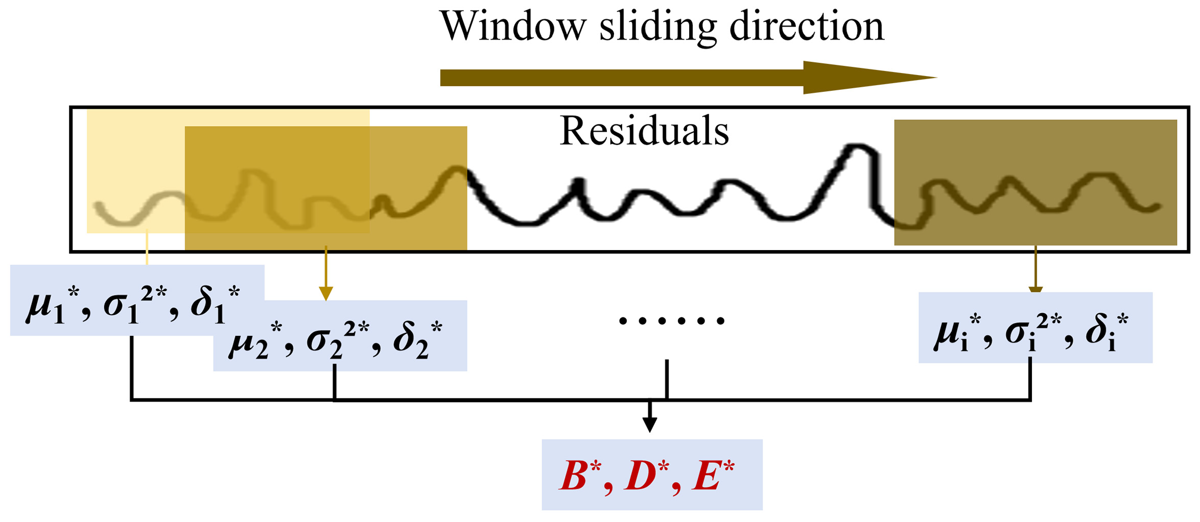
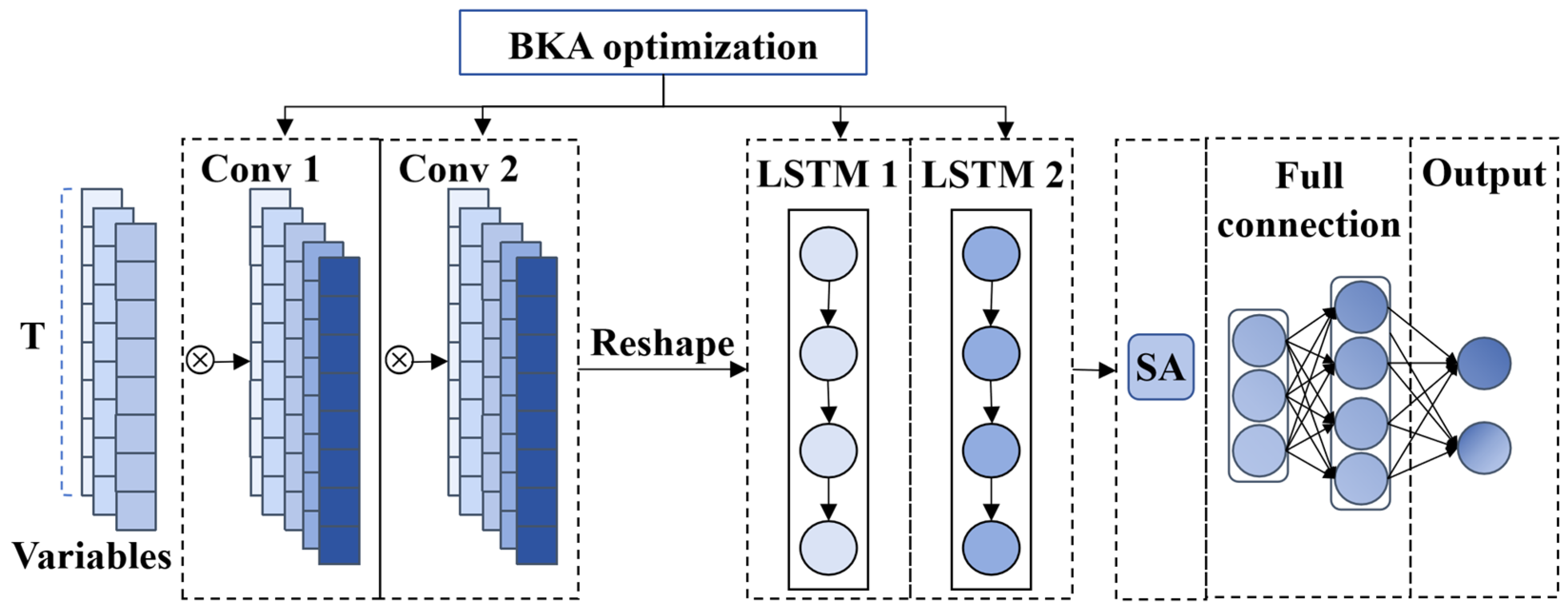
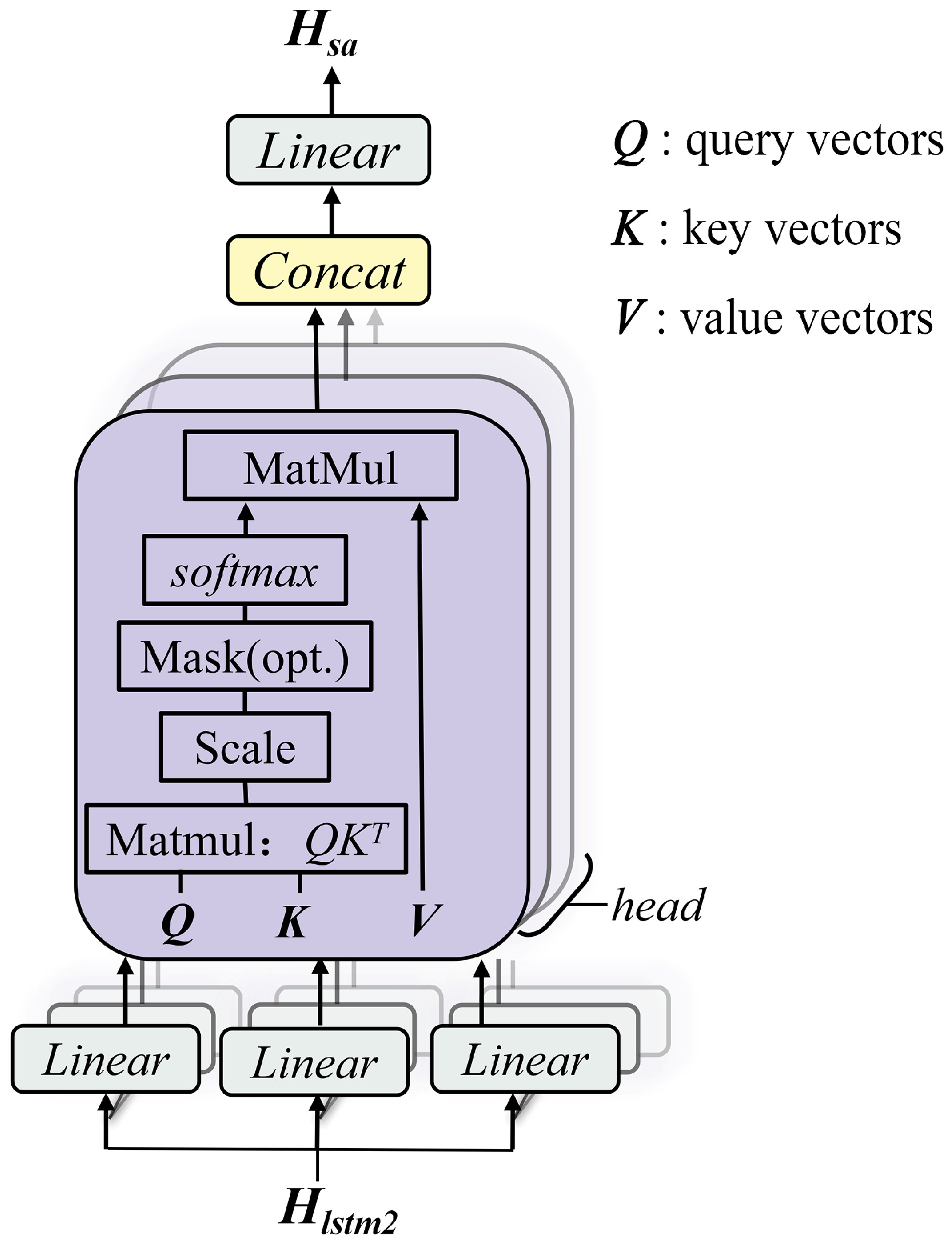
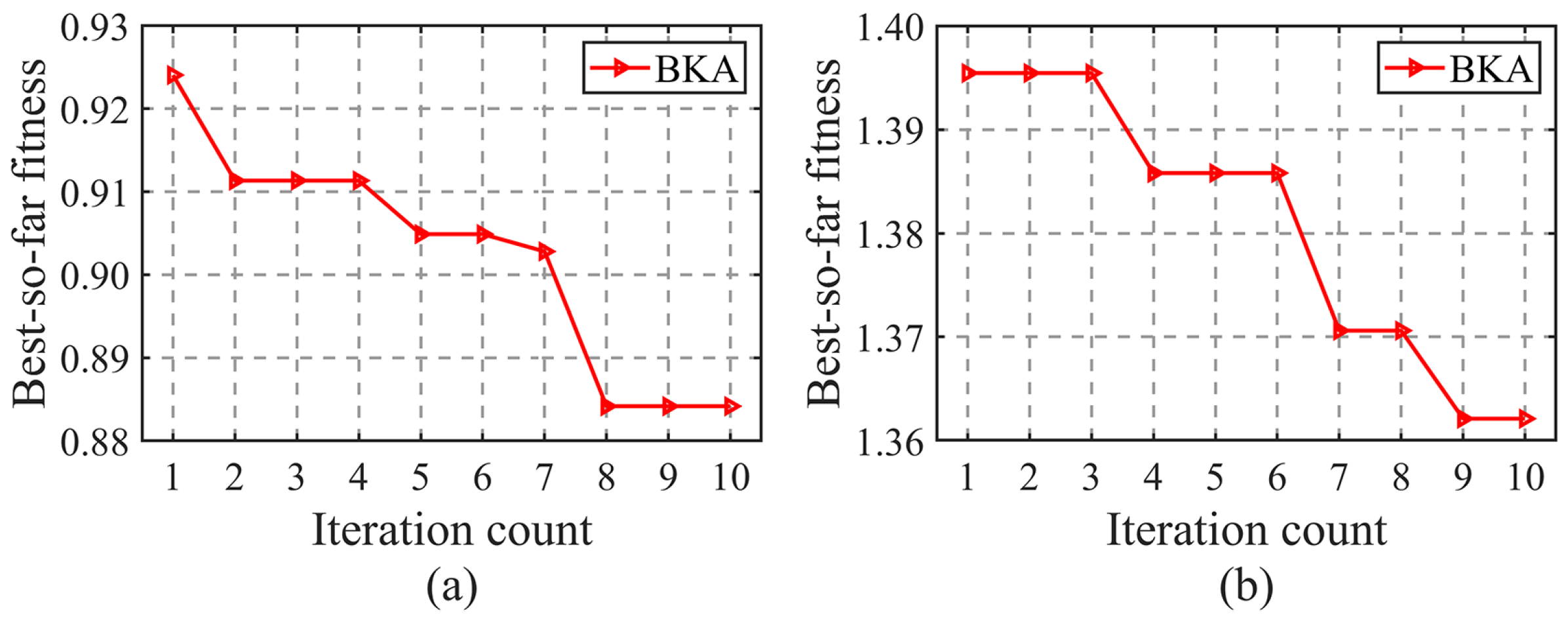
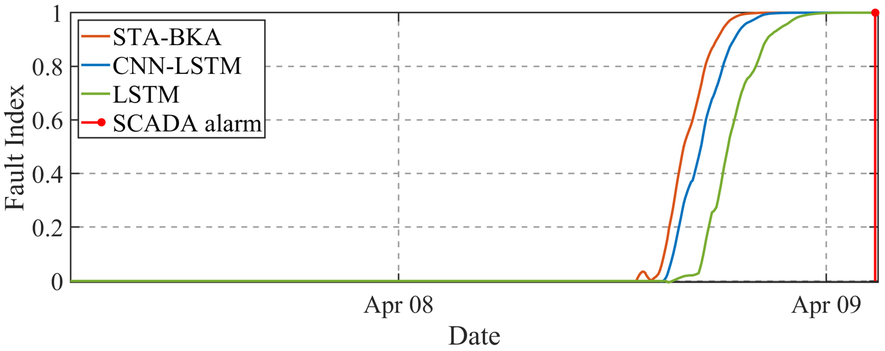
The STA-BKA model’s significant performance is anchored in its targeted resolution of three core SCADA prognostics challenges. First, its hybrid architecture overcomes the limitations in spatio-temporal modeling: convolutional layers capture multi-scale interactions among the. monitored variables, while attention-augmented LSTMs preserve long-term dependencies in low-frequency data. Second, BKA optimization prevents overfitting by balancing global–local hyperparameter tuning, enhancing noise robustness. Critically, the FI dynamically validates deviations via residual statistics in sliding windows, avoiding false alarms from fixed thresholds. This synergy explains the model’s reliable early warnings under environmental noise.

This work bridges a critical gap in wind turbine prognostics. The proposed architecture enables the accurate prediction of the GHSST and forthcoming failures, which were previously unattainable via SCADA threshold systems. By unifying spatio-temporal modeling with SA and BKA optimization, it offers a hardware-free solution scalable to existing wind farms.

It is worth noting that the model’s performance under extreme weather events (e.g., blizzards or cold waves) remains unverified. Since the SCADA dataset from operational wind farms lacks sufficient samples of such rare events, due to the limited monitoring duration and geographical coverage, further validation is needed for these scenarios. Future work will employ transfer learning to fine-tune the pretrained model when extreme-condition data becomes available, enhancing its generalization capability. When dealing with larger-scale dataset, the proposed architecture will need to be upgraded with additional enhancements, such as more systematic parameter initialization methods.

7. Conclusions

In this study, we proposed a hybrid deep learning framework integrating multidimensional data cleansing, a spatio-temporal attention network, and dynamic fault indicator, for early fault detection in wind turbine gearboxes. It has been validated that the proposed method significantly improves the fault prediction accuracy and enhances the adaptability of early warning mechanisms.

The key contributions of this study are as follows:

• Comprehensive multidimensional anomaly cleansing: A systematic anomaly classification and cleansing strategy was developed based on the distributional characteristics and root causes of different types of anomalies. The refined WSP curves exhibit smooth and concentrated distributions, verifying the effectiveness of the proposed approach in removing diverse outliers. This high-quality data foundation is crucial for improving the reliability of subsequent modeling.
• Enhanced spatiotemporal modeling: The STA-BKA model effectively captures the complex interactions among SCADA variables. By integrating hierarchical convolutional spatial feature extraction, LSTM-based temporal dependency modeling, and a multi-head attention mechanism, the model significantly enhances the temperature prediction accuracy. Compared to conventional single models, the proposed method reduces the RMSE by 37%, demonstrating a superior modeling capability for gearbox temperature dynamics.
• Adaptive fault-warning mechanism: The FI dynamically adjusts to operational condition fluctuations, overcoming the limitations of fixed-threshold alarms. This approach enables early fault detection 7–16 h before conventional SCADA alarms, significantly improving the timeliness and reliability of gearbox fault warnings.

Overall, this study provides a quantifiable, cost-effective, and scalable solution for wind turbine gearbox health monitoring, contributing to improved operational safety and reduced maintenance costs. Future research will focus on extending its applicability to other wind turbine components.