Article

Efficient Prediction of Shallow-Water Acoustic Transmission Loss Using a Hybrid Variational Autoencoder–Flow Framework

School of Marine Technology, Ocean University of China, Qingdao 266100, China
*
Author to whom correspondence should be addressed.
J. Mar. Sci. Eng. 2025, 13(7), 1325; https://doi.org/10.3390/jmse13071325
Submission received: 26 May 2025 / Revised: 28 June 2025 / Accepted: 8 July 2025 / Published: 10 July 2025
(This article belongs to the Special Issue Data-Driven Methods for Marine Structures)

Abstract

Efficient prediction of shallow-water acoustic transmission loss (TL) is crucial for underwater detection, recognition, and communication systems. Traditional physical modeling methods require repeated calculations for each new scenario in practical waveguide environments, leading to low computational efficiency. Deep learning approaches, based on data-driven principles, enable accurate input–output approximation and batch processing of large-scale datasets, significantly reducing computation time and cost. To establish a rapid prediction model mapping sound speed profiles (SSPs) to acoustic TL through controllable generation, this study proposes a hybrid framework that integrates a variational autoencoder (VAE) and a normalizing flow (Flow) through a two-stage training strategy. The VAE network is employed to learn latent representations of TL data on a low-dimensional manifold, while the Flow network is additionally used to establish a bijective mapping between the latent variables and underwater physical parameters, thereby enhancing the controllability of the generation process. Combining the trained normalizing flow with the VAE decoder could establish an end-to-end mapping from SSPs to TL. The results demonstrated that the VAE–Flow network achieved higher computational efficiency, with a computation time of 4 s for generating 1000 acoustic TL samples, versus the over 500 s required by the KRAKEN model, while preserving accuracy, with median structural similarity index measure (SSIM) values over 0.90.

1. Introduction

Acoustic waves serve as the sole effective medium for long-distance information transmission in marine environments, playing a crucial role in modern underwater communication and sensing applications. In shallow water regions, acoustic propagation primarily manifests as a complex waveguide phenomenon, governed by the coupling between dynamic oceanographic variables and boundary interactions. Acoustic transmission loss (TL) stands out as a key quantity in underwater acoustics for characterizing acoustic propagation. Conventional physics-based approaches for underwater TL prediction rely on numerical solutions, such as KRAKEN based on normal mode [1], and BELLHOP based on ray tracing [2]. However, these methods inevitably demand intensive recalculations for each new scenario, limiting their efficiency in generating massive datasets.
In contrast, deep learning offers a data-driven alternative with strong nonlinear mapping capabilities, enabling accurate input–output approximation and batch processing of large-scale datasets, thereby eliminating the need for recalculations. Critically, this advantage has been exploited in recent advances across underwater acoustics, particularly through two paradigms: (i) deep generative augmentation methods, and (ii) supervised surrogate models. The first paradigm leverages deep generative models to learn the probability distribution of underwater acoustic data through latent variables, swiftly generating synthetic samples that statistically indistinguishable from empirical observations. Notably, variational autoencoders (VAEs) [3], renowned for their training stability and explicit low-dimensional representations, have proven effective in generating underwater acoustic channel impulse responses (CIRs) samples for data augmentation [4]. Furthermore, generative adversarial networks (GANs) [5] have demonstrated remarkable efficacy in underwater acoustic data augmentation due to their capability for producing high-fidelity synthetic samples. Liu et al. [6] employed a conditional generative adversarial network (CGAN) to synthesize cross-spectral features from image representations, which improves source ranging accuracy through enhanced feature generation. Similar extensions using GAN architectures [7,8,9] have further validated this paradigm’s effectiveness in data augmentation, where synthetic sample generation substantially enhances downstream task performance through dataset expansion. However, this approach operates as an unsupervised framework, lacking explicit input–output mapping capabilities, thus limiting controllable scenario-specific prediction.
Unlike generative models that learn data distributions, the second paradigm employs supervised deep neural networks as surrogate models to learn deterministic input-output mappings, enabling efficient controllable prediction. Varon et al. [10] trained a deep neural network as a surrogate model to predict modal wavenumbers and group speeds across diverse environments, replacing computationally intensive normal mode simulations and enabling rapid TL calculation. Subsequent developments employed specialized architectures as surrogates for TL prediction. Mallik et al. [11] used a convolutional recurrent autoencoder network (CRAN), while Sun et al. [12] developed a Multi-Scale-DUNet for TL field prediction across varied source conditions. Nevertheless, these supervised surrogate models depend on extensive labeled data and exhibit a performance tied to the training data distribution, and significant deviations in unseen test conditions may trigger accuracy degradation.
While deep generative augmentation methods learn data distributions for enhanced generalization, they inherently lack controllability. Conversely, supervised surrogate models enable scenario-specific prediction, but their generalization to unseen conditions may be constrained by training data convergence. To develop rapid prediction model mapping of sound speed profiles (SSPs) to acoustic TL through controllable generation, this study advances the first paradigm by introducing a hybrid variational autoencoder–normalizing flow (VAE–Flow) framework through a two-stage training strategy. The framework specifically employs (1) a VAE to learn latent representations of TL data on a low-dimensional manifold, and (2) a normalizing flow to establish bijective mapping between latent variables and physical parameters. This approach addresses the controllability limitation of the first paradigm by reinforcing variable mappings through the integration of a normalizing flow. Combining the trained normalizing flow with the VAE decoder can establish an end-to-end mapping from SSPs to TL, achieving prediction speeds surpassing the conventional KRAKEN model.

2. Method

This section proposes a hybrid framework for TL prediction, comprising a VAE and a normalizing flow: the VAE learns low-dimensional representations of acoustic TL data through latent variables, while the normalizing flow establishes a bijective mapping between the latent space and physical parameters, achieving end-to-end mapping from physical parameters to TL.

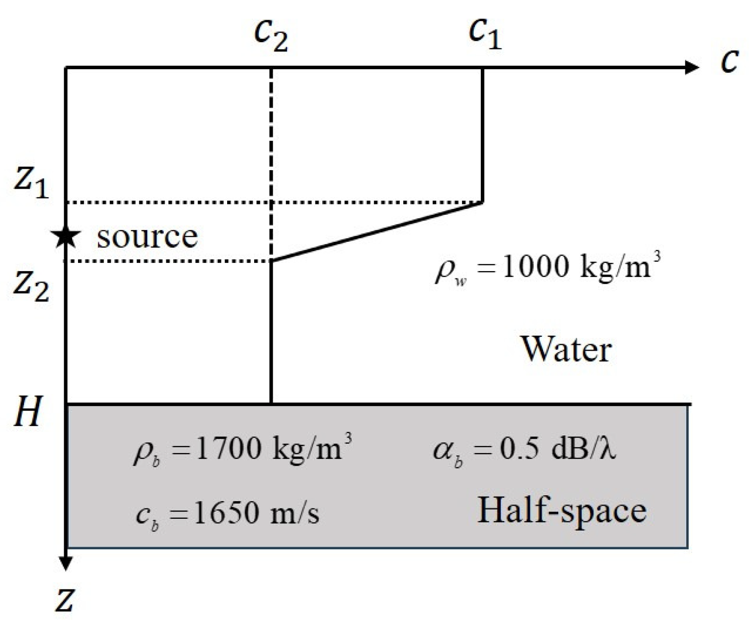
2.1. Problem Description

For a point source of angular frequency ω positioned at depth z s , the acoustic pressure field at depth z and horizontal distance r can be expressed as a sum of normal modes [13]:
p r , z e i π / 4 ρ z s 8 π r m = 1 Ψ m z s Ψ m z e i k r m r k r m r ,
where ρ ( · ) represents the medium density, k r m is the mth mode wavenumber, and Ψ m z denotes the mth modal depth function.
The outcome p r , z describes a two-dimensional spatial distribution of acoustic pressure, characterized as a complex-valued field that incorporates both magnitude and phase. In underwater acoustics research, TL is typically used for analyzing the spatial distribution of the acoustic field. Such TL can be computed from p r , z at a given receiver location ( r , z ) with respect to the reference pressure p 0 :
T L ( r , z ) = 20 log p ( r , z ) p 0 ( r = 1 ) ,
where p 0 ( r ) = e i k 0 r / 4 π r is the acoustic pressure for the source in free space.
In complex ocean environments, TL is influenced by multiple factors, including the sound speed profile, seabed topography, and the source properties, among others. By parameterizing these influencing factors into a parameter vector Θ , the transmission loss field T L R N , obtained by discretizing the receiver region ( R , Z ) into N spatial points, can be formally expressed through the forward mapping:
F : R r R N , Θ T L .
The physical parameter vector Θ R r comprises r variables representing environmental properties and source conditions. Each component in Θ = Θ 1 , Θ 2 , , Θ r T quantifies a distinct physical factor governing acoustic propagation.
In underwater acoustics, KRAKEN, as a conventional numerical model for computing low-frequency acoustic fields in shallow-water environments, has been widely recognized for its accuracy and reliability in calculating TL and serves as an alternative model for generating datasets in the absence of experimental data. By configuring the parameter vector Θ , KRAKEN effectively computes the acoustic field for the parameterized scenario and outputs the acoustic TL field via Equation (2). Nevertheless, when generating large-scale TL samples across high-dimensional parameter spaces, KRAKEN exhibits a fundamental limitation: any variation in Θ components necessitates recomputing k r m and Ψ m z through numerical solvers. This results in prohibitive computational costs, rendering it impractical for efficient generation of massive sample sets.
To address this computational constraint, this study aimed to develop a surrogate model mapping SSPs to acoustic TL through controllable generation and achieved the following functionality:
(1) Forward modeling: The model learns a mapping G : Θ T L that approximates F with high fidelity, while enabling swift prediction.
(2) Probabilistic sampling: By learning the TL data distribution, the model generates samples statistically indistinguishable from observations, with p m o d e l ( T L ) p g t ( T L ) .

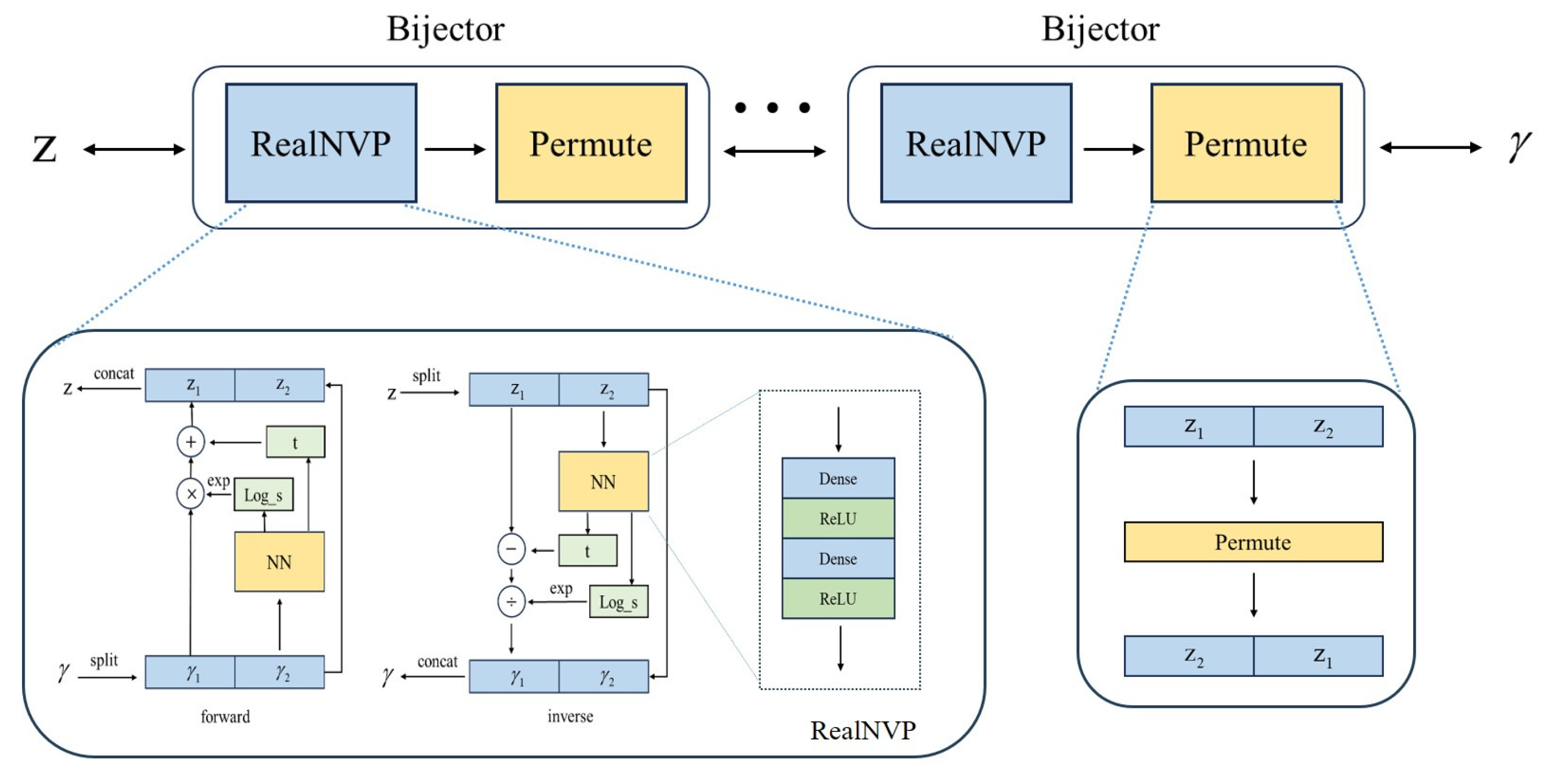
2.2. VAE–Flow Framework

To properly frame our solution, it is necessary to briefly review the manifold learning principles underlying the proposed objective. Since TL represents the spatial distribution of acoustic wave energy, the data inherently exhibit a high-dimensional structure. But it should be emphasized that the high-dimensional TL data do not uniformly populate the ambient N-dimensional space [14]. Under the manifold hypothesis, these observations reside on an r-dimensional manifold χ R N ( r N ), where r corresponds to the intrinsic dimensionality of the physical parameter space R r , and μ g t denotes the ground-truth probability measure within χ . As shown in Figure 1, a 2D physical parameter space forms a low-dimensional manifold embedded in the high-dimensional observation space.
Consequently, achieving controllable generation for rapid TL prediction, while meeting the functional requirements outlined in Section 2.1, basically necessitates
(1) Learning low-dimensional representations of TL data through encoding–decoding, where the latent space dimensionality d matches the intrinsic dimension r of the data manifold.
(2) Accurately capturing the ground-truth measure μ g t supported on the manifold χ and approximating a homeomorphism between the latent space and the manifold.
To address these modeling requirements, we developed a hybrid VAE–Flow framework through a two-stage training strategy, comprising both data generation and model training, as illustrated in Figure 2. To begin with, the KRAKEN model is employed to construct underwater TL datasets under varying SSPs for subsequent model training. Subsequently, during the model training, the framework was further decomposed into two distinct stages: First, a VAE was trained to learn latent representations of TL data on a low-dimensional manifold, while high-fidelity TL fields reconstruction could be achieved by sampling from the learned latent variable distributions and then passing them through the trained decoder. Second, a normalizing flow was independently optimized to establish a bijective mapping between the learned latent variables and the corresponding physical parameters of the simulated TL datasets. Ultimately, combining the trained normalizing flow with the VAE decoder established an end-to-end mapping from physical parameters to predicted TL.
Before proceeding further, it is essential to examine the theoretical foundations of this framework through the lens of VAEs and normalizing flows, with specific attention to two key aspects:
(1) Why is the model training stage divided into two separate phases?
(2) What are the functional contributions of the VAE and Flow network within each phase?
We employed VAE as our first-stage model due to its encoder–decoder architecture for effective low-dimensional representation learning. As a likelihood-based deep generative model, the VAE fundamentally performs maximum likelihood estimation (MLE) for data modeling [15]:
θ ^ = arg max θ log p θ ( x ) ,
where the observed data x are assumed to be independently and identically distributed, and p θ ( x ) is the probability density function parameterized by θ . However, the integral of the marginal likelihood p θ ( x ) = p θ ( x | z ) p ( z ) d z is intractable. The VAE addresses this by introducing a recognition model q ϕ ( z | x ) to approximate the true posterior p θ ( z | x ) , where ϕ can be viewed as tuning the degree of approximation. Under this framework, the log-likelihood objective of MLE can be decomposed as follows:
log p θ ( x ) = L ( θ , ϕ ; x ) + D K L [ q ϕ ( z | x ) | | p θ ( z | x ) ] .
Here, D K L [ · ] represents the Kullback–Leibler (KL) divergence measuring the discrepancy between q ϕ ( z | x ) and p θ ( z | x ) . Since KL divergence is non-negative, the first RHS term is called the Evidence Lower Bound (ELBO), and Equation (5) can be written as
log p θ ( x ) L ( θ , ϕ ; x ) = E z q ϕ ( z | x ) log p θ ( x | z ) D K L q ϕ ( z | x ) | | p ( z ) ,
with equality iff q ϕ ( z | x ) = p θ ( z | x ) (i.e., when D K L [ · ] equals zero, the ELBO becomes tight). Here, E · represents the mathematical expectation operator, and p ( z ) is the prior over latent variables z. In Equation (6), q ϕ ( z | x ) functions as an encoder, while p θ ( x | z ) acts as a decoder, both are commonly specified as Gaussians. By introducing latent variables and the reparameterization trick, the VAE enables optimization of the following objective function:
L ( θ , ϕ ; x ) = χ 1 L l = 1 L log p θ ( x | z ( l ) ) + D K L [ q ϕ ( z | x ) | | p ( z ) ] μ g t d x z ( l ) = μ z + Σ z 1 / 2 ε ( l ) ,
where ε represents a random variable sampling from N ( 0 , I ) and L denotes the total number of random samples.
Through neural network optimization of this objective function, the VAE learns latent representations of the data. While sampling from the latent space and passing through the decoder enables data synthesis, this generation process remains uncontrolled. The core limitation stems from VAE’s construction of the density function p θ ( x ) in the full-dimensional observation space, despite the data manifold having a lower intrinsic dimensionality. This mismatch prevents the model from learning the ground-truth probability measure on the manifold, even when the objective function (ELBO) is maximized. Mathematically, this implies that p θ ( x | z ) maps all samples from q ϕ ( z | x ) to the correct manifold with a trivial reconstruction error for any x χ , but the measure μ g t on χ has not been accurately estimated:
q ϕ ( z ) χ q ϕ ( z | x ) μ g t dx R N p θ ( z | x ) p θ ( x ) dx = p ( z ) .
Here, q ϕ ( z ) represents the aggregated posterior in the latent space, which errantly deviates from the prior distribution p ( z ) . This may lead to p θ ( x | z ) generating samples outside the data manifold when z p ( z ) , as the decoder operates in ambient space, while the data lie on χ .
To address this limitation, Daibin et al. [16] proposed a Two-Stage VAE, later generalized by Loaiza-Ganem et al. [17] as Two-Step Models. The essential of such methods lies in (i) first learning low-dimensional representations through an encoder–decoder architecture where the latent space dimensionality matches the intrinsic manifold dimension, ensuring the latent variables sampled from this space exhibit non-zero measure across the full ambient space R r ; (ii) training a second deep generative model on this properly aligned latent space to capture the manifold’s ground-truth probability measure [18]. While Daibin et al.’s approach employs two independent VAEs for higher quality image generation, we propose replacing the second-stage VAE with a normalizing flow to better satisfy the functional requirements of controllable generation, making it more suitable for TL prediction tasks. Consequently, a brief introduction to the principles of normalizing flows is warranted here.
Originally proposed by Rezende et al. [19], normalizing flows operate based on the core idea of exact distributional mapping via invertible variable transformations. For instance, to achieve bijective mapping between the original distribution p ( u ) and the latent distribution p ( v ) , normalizing flows construct a series of multivariable bijective functions f : R D R D . This allows
u = f ( v ) v = f 1 ( u ) .
The probability densities are preserved through a change in the variable formula:
p ( u ) = p ( v ) det d v d u = p ( v ) det J ( f 1 ( u ) ) .
Here, J denotes the Jacobian matrix comprising all first-order partial derivatives. Thus, normalizing flows enable exact computation of the log-likelihood in MLE by evaluating the Jacobian determinant during variable transformation, as formalized below:
log p ( u ) = log p ( v ) i = 1 K log det d f i d v i 1 ,
where K denotes the total number of multivariable bijective functions constituting the transformation sequence. Crucially, normalizing flows enable exact probability density estimation through invertible transformations, and precise bijective mapping between variable distributions [20]. These properties make normalizing flows better suited than VAEs for controllable generation tasks.
Building upon the theoretical foundations, we now address the two previously posed research questions. Our hybrid framework achieves controllable generation by training a VAE and a normalizing flow separately: (1) Training a VAE to learn low-dimensional TL representations with latent space dimensionality aligned to the dimensionality of empirical orthogonal functions (EOF) coefficients (detailed in Section 3.1), ensuring full-dimensional coverage in R r , while minimizing the reconstruction error; (2) Optimizing a normalizing flow to establish a bijective mapping between latent variables and EOF coefficients, which is equivalent to minimizing D K L ( q ϕ ( z ) | | p ( z ) ) , thereby learning the ground-truth probability measure on the manifold. Through two-stage training, the VAE–Flow framework essentially approximates a homeomorphic mapping between latent and physical parameter spaces, thereby enhancing the controllability of the generation process and establishing a forward mapping from SSPs to TL fields.
Notably, while existing studies [19,21] combined VAEs with normalizing flows, their objectives differed from ours. These works primarily employed normalizing flows to enhance the variational posterior approximation, replacing the standard Gaussian assumption with more flexible, complex distributions to improve image generation quality:
L = E z 0 q 0 log p ( x | z k ) D K L q k ( z k ) p ( z )
In Equation (12), z 0 is the initial Gaussian latent variable from the encoder, while z k is its transformed version through normalizing flows. However, these methods are not designed to establish an effective bijective mapping, rendering them unsuitable for controllable generation. By contrast, our framework decomposes the optimization into two dedicated stages, which ensures each model specializes in its target function, while eventual integration enables controllable generation. The complete procedure for the hybrid VAE–Flow framework can be summarized as follows:
(1) Given physical parameters Θ ( i ) i = 1 M drawn from a prior distribution p ( Θ ) , compute the corresponding acoustic TL fields via KRAKEN, obtaining M simulation samples T L ( i ) i = 1 M .
(2) Train a VAE, with the latent space dimension set equal to the dimensionality of the physical parameters, to learn the manifold structure underlying the acoustic TL data (the reconstruction error between the decoder’s output and ground truth is minimized). Generate latent variables z ( i ) i = 1 M via z ( i ) q ϕ ( z | T L ( i ) ) , which approximately follow a distribution but are unlikely to match p ( Θ ) .
(3) Train an additional normalizing flow, take the samples z ( i ) i = 1 M as input, to learn a bijective mapping between q ( z ) and p ( Θ ) .
(4) Upon completion of training, end-to-end prediction from physical parameters to acoustic TL can be achieved via Θ * p ( Θ ) , z * = f 1 ( Θ * ) , and T L * p θ ( T L | z * ) .
Based on this theoretical framework, we further construct a VAE–Flow network in Section 3 to achieve rapid prediction of acoustic TL under different SSPs.

3. Method Implementation

This section details the implementation of the VAE–Flow framework, including data generation procedures, the VAE–Flow network architecture, training configurations, and evaluation metrics for controllable TL prediction.

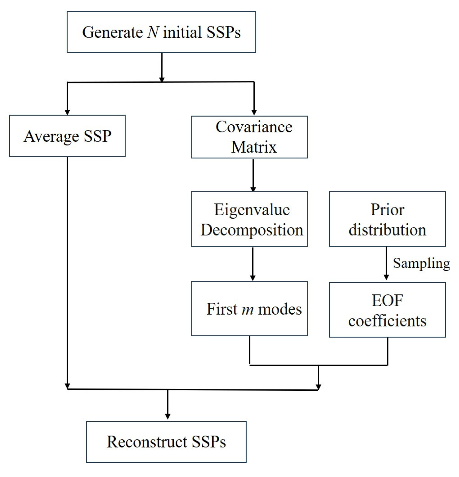
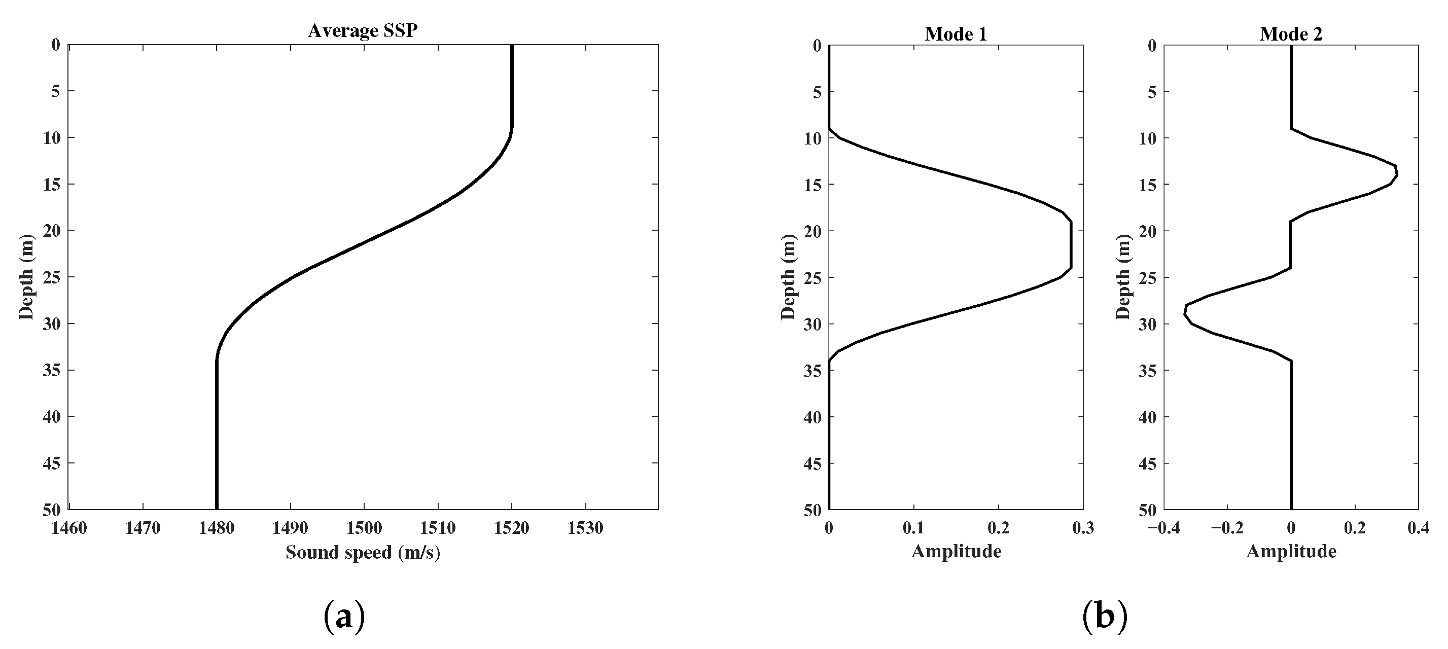
3.1. Dataset Generation Procedures

In shallow-water environments, the propagation characteristics of acoustic waves are influenced by multiple environmental factors, with the sound speed profile serving as a critical parameter that characterizes the temporal and depth-dependent variations in sound speed in seawater. As a fundamental component for constructing acoustic propagation models, the SSP directly determines acoustic wave propagation paths and velocities, making it an essential environmental parameter for accurate sound field modeling. This study primarily focuses on the influence of SSP on acoustic propagation. Given the scarcity of underwater experimental data, we generated simulated acoustic TL data via the KRAKEN model under various SSPs to construct the training dataset for our network.
As illustrated in Figure 3, a typical shallow-water waveguide with a negative thermocline is parameterized by water depth, density, SSP, and seabed acoustic properties. In this case, the water depth H was 50 m, with the source depth z s fixed at 25 m. The water density ρ w was 1000 kg/m3, and the sound speed was characterized by a negative thermocline profile, with an upper-layer sound speed c 1 of 1520 m/s and a lower-layer sound speed of 1480 m/s, while compressional wave attenuation in the water column was neglected. The seabed was modeled as an infinite half-space with a sound speed c b of 1650 m/s, a density ρ b of 1700 kg/m3, and an absorption coefficient α b of 0.5 dB/ λ . The sea surface was modeled as a pressure–release boundary, with water mass movements excluded during the simulations. During data generation, we employed the waveguide environment illustrated in Figure 3, with the aforementioned parameters serving as the baseline configuration for the KRAKEN simulations.
To generate a large-scale dataset of acoustic TL, this paper employed the empirical orthogonal function (EOF) method to reduce the dimensionality and reconstruct SSPs. Multiple SSPs were generated through this approach for acoustic TL computation and dataset construction, with the detailed workflow illustrated in Figure 4. Since the eigenvectors obtained from eigenvalue decomposition of a sound speed covariance matrix are mutually orthogonal, the first m dominant modes with high energy contribution rates can be selected for SSP reconstruction:
c = c 0 + i = 1 m a i f i .
where c 0 represents the average sound speed profile, f i denotes the i-th order EOF mode, and a i is the corresponding i-th EOF coefficient.
The generation process began by creating N initial sound speed profiles through random perturbations, wherein the upper-layer depth of the negative thermocline z 1 was randomly sampled 100 times across [10 m, 30 m], and the lower-layer depth z 2 was defined as z 2 = z 1 + h (with h = 15 m). Upon subjecting these 100 profiles to EOF decomposition, the variance contribution rates of the first five modes were quantified as 95.31 % , 3.90 % , 0.49 % , 0.13 % , and 0.06 % , respectively, revealing that the first two modes dominated 99.21 % of the total energy. Consequently, these two modes were selected for profile reconstruction in this section, with their spatial distributions and the average sound speed profile illustrated in Figure 5. To align with the proposed modeling framework, the EOF coefficients had to adhere to specific probability distributions during reconstruction, which was implemented by sampling from two independent priors to generate M coefficient sets. It can be established that the physical degrees of freedom for both SSPs and acoustic TL field data were determined by the dimensionality of the EOF coefficients.
This study assumed these two EOF coefficients followed Gaussian distributions, specifically a 1 N ( μ 1 , σ 1 2 ) and a 2 N ( μ 2 , σ 2 2 ) . For computational convenience, we set μ 1 = μ 2 = 0 and defined six distinct standard deviation values, constructing the dataset as presented in Table 1. For each EOF parameter set, we sampled 6000 data points and generated 6000 corresponding SSPs using Equation (13). Subsequently, the SSPs corresponding to the six datasets were utilized as environmental parameters in KRAKEN to compute the sound field, where the source frequency was uniformly set to 200 Hz, and the simulated area covered a horizontal range of 1–10 km ( Δ r = 10 m) and a vertical range of 1–50 m ( Δ z = 1 m). This process yielded six groups of acoustic TL data matrices T L ( M , r , z ) R 6000 × 901 × 50 . Each TL sample was subsequently converted into an RGB image with pixel dimensions of 256 × 256 × 3 , where 256 × 256 represents the image resolution and 3 denotes the color channels (red, green, and blue). Thus, six distinct sets of TL image datasets, each determined by different EOF coefficient distributions, were further used to train the VAE–Flow network. It should be noted that TL was selected as the input for two key reasons: First, neural networks are sensitive to the numerical distribution of input data during training, and TL exhibits a relatively constrained dynamic range that mitigates the training instability caused by magnitude disparities. Second, compared to 1D features, TL representations provide a more comprehensive characterization of acoustic wave propagation in spatial domains. Furthermore, by formatting the data as RGB images, we could fully leverage the inherent advantages of convolutional neural networks in feature extraction, thereby significantly enhancing the model’s learning capacity.

3.2. VAE–Flow Network Architecture

To enable rapid prediction of shallow-water acoustic TL, a VAE–Flow network was constructed based on the modeling framework proposed in Section 2. In this architecture, the VAE network is employed for learning the latent representations of the acoustic TL fields, while achieving high-fidelity TL reconstruction, whereas the Flow network serves to establish a bijective mapping between the learned latent variables distribution and the target distribution of the EOF coefficients. As previously established in Section 2, these two training phases are mutually independent. Given that the acoustic TL datasets consisted of RGB images with pixel resolution, this section incorporated convolutional layers and residual blocks into the fundamental VAE. These enhancements were implemented to improve the network’s feature extraction capability for image data, and to mitigate potential gradient vanishing issues.
The architecture of the VAE network developed in this paper is illustrated in Figure 6. In accordance with the VAE principles, the network consists of encoder and decoder components. The encoder comprises an initial downsampling module, five residual blocks and a mapping module, while the decoder is composed of a projection module, seven residual blocks, and an output module. Considering the capability of convolutional layers in capturing the intrinsic characteristics of data, we selected them as the core component for feature extraction. The initial downsampling module of the encoder consists of a 7 × 7 convolutional layer, followed by batch normalization and the LeakyReLU activation function. Additionally, a max pooling layer is also attached to reduce the spatial dimensions of the feature maps. It should be noted that the encoder incorporates several residual blocks, which originate from the classical ResNet [22]. Each residual block consists of two repetitive units containing a 3 × 3 convolutional layers, batch normalization, and a LeakyReLU activation function. Crucially, a skip connection directly sums the input to the feature map before the final LeakyReLU activation function, which mitigates vanishing gradients via identity shortcut paths. Moreover, compared to the first block, the residual block introduces an additional linear transformation ( 1 × 1 convolutional layer), as shown in Figure 6, specifically designed to address the dimensional mismatch between inputs and outputs caused by downsampling operations. Following this, the mapping module employs a global average pooling layer to reduce the spatial dimensions of the feature maps to 1 × 1 , subsequently branching into two parallel dense layers that output the mean μ z and standard deviation Σ z 1 / 2 parameters of the latent distribution. Through the implementation of this architecture, the encoder learns to map high-dimensional acoustic TL images into a low-dimensional latent space during training, while outputting μ z and Σ z 1 / 2 of the latent variables to represent the learned underlying distribution.
In the decoder, the projection module first upsamples the latent variable z through a dense layer followed by a ReLU activation function, then reshapes the vector back into feature maps. The residual blocks in the decoder maintain the same architecture as those in the encoder, except that the 3 × 3 convolutional layers are replaced with 3 × 3 transposed convolutional layers to achieve feature map upsampling. Finally, the output module reconstructs the features into 256 × 256 × 3 images, representing the generated acoustic TL fields.
Since the latent distribution learned by the VAE network exhibited discrepancies with the EOF coefficients distribution, this study used the additional incorporation of a normalizing flow network to further refine the distribution fitting. In recent years, normalizing flows have evolved significantly, giving rise to a series of influential architectures, including NICE [23], RealNVP [20], Glow [24], and TARFLOW [25]. Building upon these advancements, we adopted the fundamental architecture of RealNVP to construct the Flow network. As illustrated in Figure 7, the network comprises multiple bijectors, each containing a RealNVP module and a permute module.
The RealNVP architecture utilizes affine coupling layers to construct exact bijective mappings through a structured transformation process. In each layer, the input vector is first partitioned along its feature dimension, with one subset undergoing nonlinear transformation via a neural network module composed of dual dense layers and ReLU activation functions that generate both scaling and translation parameters (s and t), while the complementary subset remains unchanged. The subsequent affine recombination of these processed and unprocessed partitions yields two critical mathematical properties: analytically tractable invertibility, due to the explicit transformation scheme, and computational efficiency, stemming from the Jacobian determinant with low complexity. The permute module serves a critical function by systematically interchanging data dimensions during both forward and inverse propagation. This dimensional rearrangement ensures comprehensive processing through the RealNVP’s affine coupling layers, guaranteeing that all data dimensions undergo transformation rather than being limited to specific subsets. Through this mechanism, the designed Flow network directly satisfies the exact density estimation requirements essential for distribution fitting within our proposed framework.

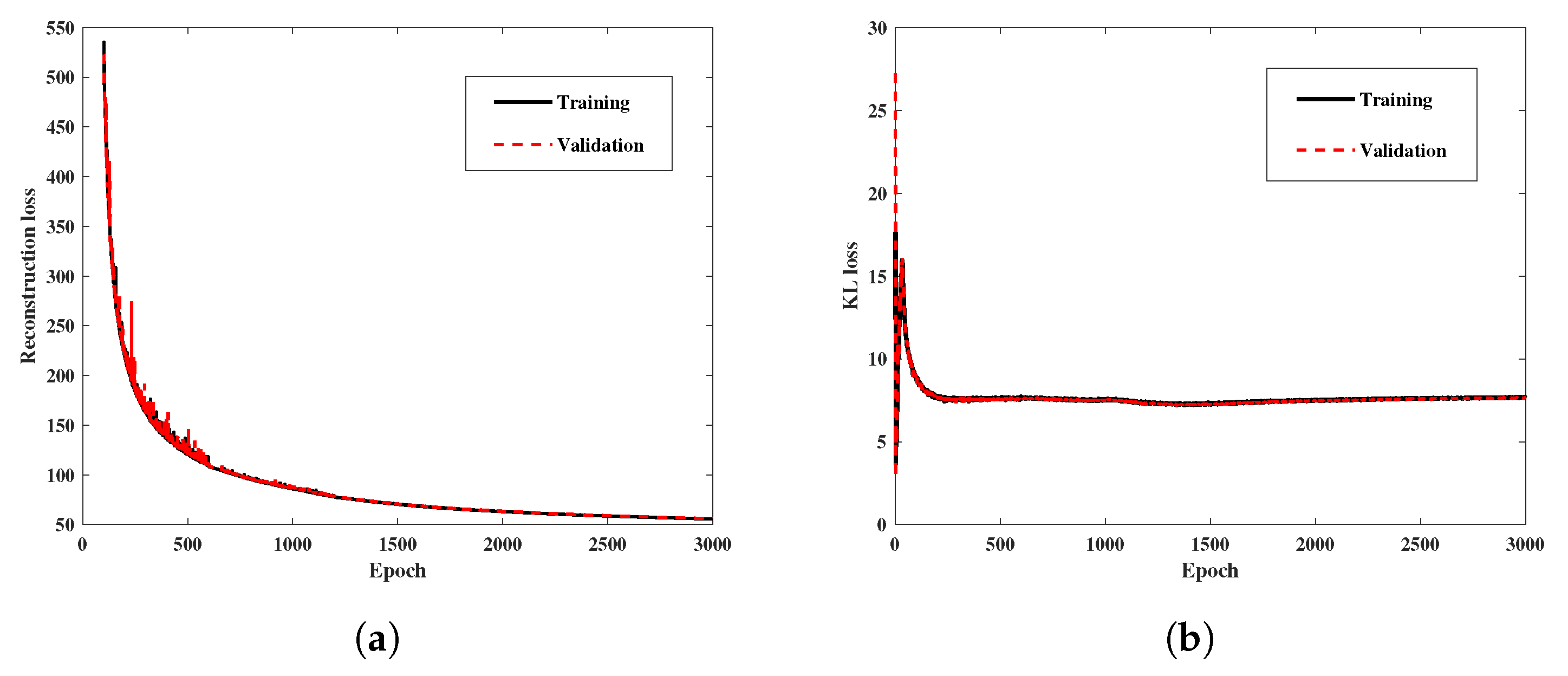
3.3. Training Configurations

3.3.1. Network Training Configuration

Since the training processes of the two networks are mutually independent and require the completion of VAE training before extracting the corresponding latent variables for subsequent Flow network training, their configurations must be differentiated. Specifically, we first constructed the VAE and Flow networks according to Section 3.2, then employed their respective objective functions (as detailed in Section 2.2) as loss functions to quantify the training performance.
For the VAE network, the latent space dimension was set to match the order of EOF coefficients (i.e., 2). Given that the input consisted of 256 × 256 × 3 RGB images requiring dimensional reduction to the latent space followed by reconstruction, the network contained substantial trainable parameters—specifically 4.9 million in the encoder and 7.2 million in the decoder. Notably, we represented the output data variance in the decoder as a hyperparameter β , using x = β I , which also underwent optimization with the objective function during training. Previous work by Daibin et al. [16] demonstrated that proper configuration of this hyperparameter is essential for achieving high-quality reconstruction in VAE models. The batch size was specified to be 256, and the initial learning rate was set to 1 × 10 4 , with the rate halved after every 1/5 of the total epochs to mitigate against training instability and avoid local optima. Upon completion of the VAE network training, the training set was projected into the latent space through the encoder to obtain corresponding latent variables, which subsequently served as inputs to the subsequent Flow network.
Since the VAE network had already performed dimensionality reduction on the original TL data, the Flow network processed low-dimensional data during training. Accordingly, the Flow network employs a series of four bijectors, each RealNVP module contains dense layers with 512 neurons, containing 3.1 million training parameters in total. Consistent with the previous training protocol, we implemented a learning rate decay mechanism with an initial rate of 1 × 10 5 , halved after every 2/5 of the total epochs, and a batch size of 64. Considering the Flow network primarily consists of dense layers, an early stopping strategy was employed to mitigate overfitting, wherein training was terminated prematurely if the validation loss failed to improve over 10 consecutive epochs. The Adam optimizer was used for both the VAE and Flow networks.

3.3.2. Computational Implementation

The deep learning training performed on a server with an Intel Xeon Platinum 8370C CPU and an NVIDIA GeForce RTX 4090, using the programming environment Python 3.9 and Tensorflow 2.10.0. Furthermore, the construction of the Flow network was implemented using Tensorflow Probability (TFP), a specialized extension library of Tensorflow, which provides optimized interfaces for efficient implementation of normalizing flows, significantly enhancing both development efficiency and computational performance.

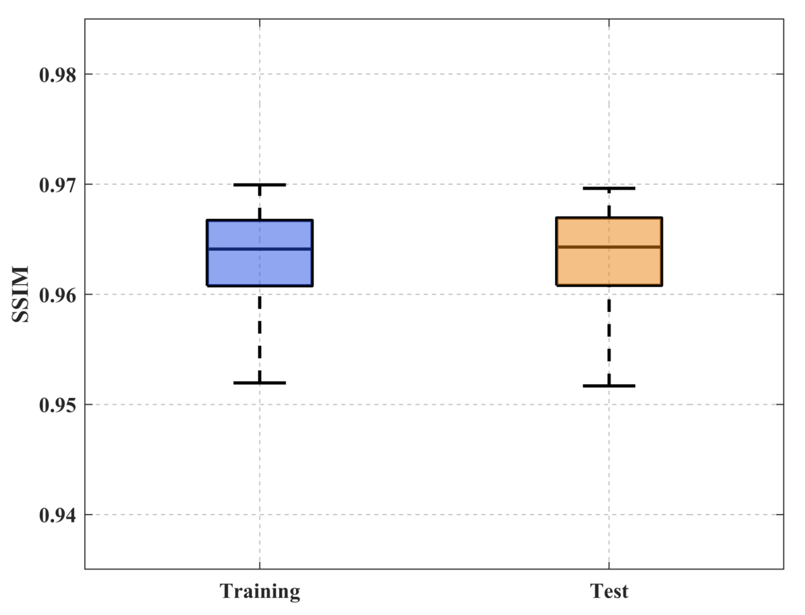
3.4. Evaluation Metrics

To evaluate the training outcomes at each stage and assess the VAE–Flow network’s generalization performance, it was necessary to introduce additional evaluation metrics beyond the loss function. This study employed the structural similarity index measure (SSIM), mean squared error (MSE), and maximum mean discrepancy (MMD) as comprehensive performance metrics. SSIM is a metric from image processing that quantifies the similarity between two images in terms of luminance, contrast, and structural characteristics. It evaluates image similarity by comparing local statistical properties of images:
S S I M ( x , x ^ ) = ( 2 μ x μ x ^ + C 1 ) ( 2 σ x x ^ + C 2 ) ( μ x 2 + μ x ^ 2 + C 1 ) ( σ x 2 + σ x ^ 2 + C 2 ) ,
where μ x and μ x ^ represent the mean intensities of the ground truth x and reconstructed (or predicted) acoustic TL field x ^ , respectively. σ x 2 and σ x ^ 2 denote the variances in x and x ^ , while σ x x ^ is the covariance between them. C 1 and C 2 are small constants introduced to prevent division by zero.
The MSE metric quantifies numerical accuracy by computing the average squared differences between corresponding elements of two matrices:
M S E ( x , x ^ ) = 1 m n i = 1 m j = 1 n ( x i j x ^ i j ) 2 .
In this study, MSE was mainly employed to evaluate the accuracy of the distribution fitting achieved by the Flow network. In parallel, MMD is a kernel-based metric designed to quantify the distributional discrepancy between two sample sets in a reproducing kernel Hilbert space (RKHS). This metric can be expressed through kernel functions:
M M D ( x , x ^ ) = 1 n 2 i = 1 n j = 1 n k ( x i , x j ) + 1 m 2 i = 1 m j = 1 m k ( x ^ i , x ^ j ) 2 n m i = 1 n j = 1 m k ( x i , x ^ j ) ,
with the present study employing a Gaussian kernel for MMD computation to measure the distributional differences between the ground truth and fitting results.

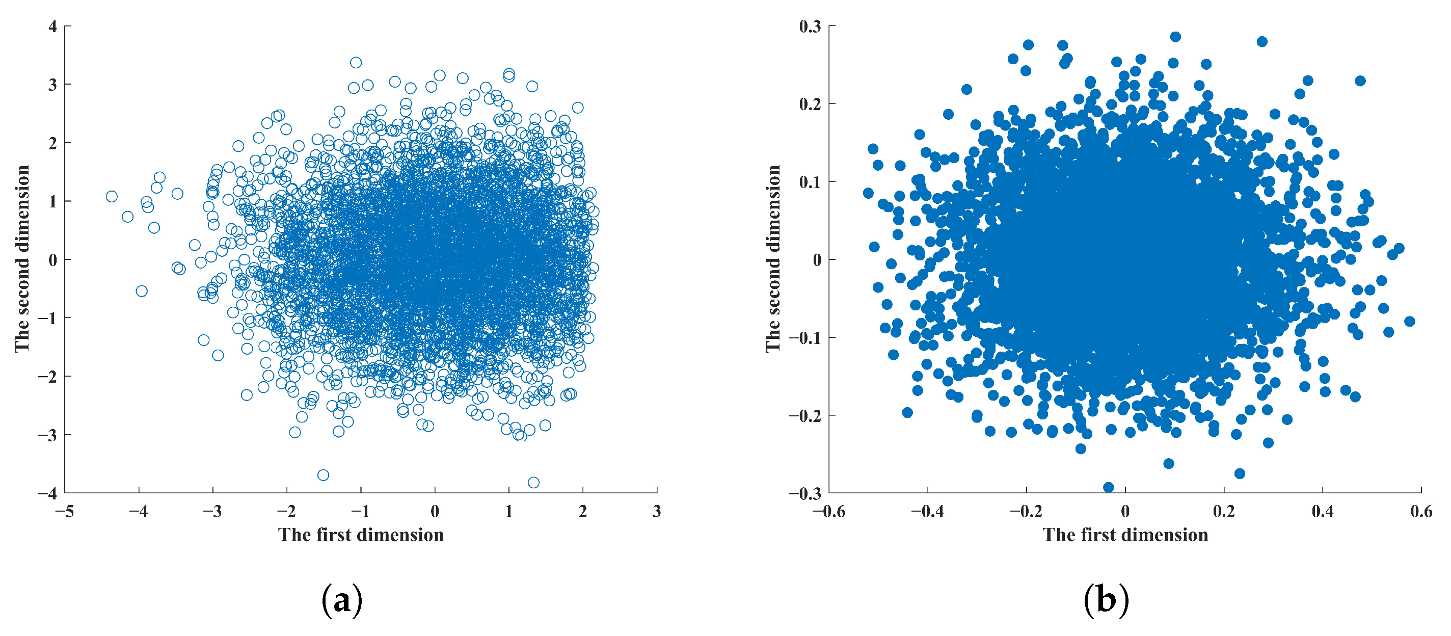
4. Evaluation and Analysis

Based on the established VAE–Flow network architecture and training settings, we first evaluated the performance of both the VAE and Flow networks using the D1 dataset generated in Section 3.1. The D1 dataset was divided into training, validation, and test sets at a ratio of 10:1:1. Initializing the hyperparameter β to 1, we trained the VAE network for 3000 epochs. Due to the hyperparameter configuration, the total loss of the VAE tended to approach negative infinity during optimization. To better analyze the convergence behavior, we decomposed the VAE’s objective function into reconstruction loss and KL divergence loss (as discussed in Section 2.2), monitoring their respective evolution throughout the training process.
Figure 8 presents the training and validation loss curves for both components. The reconstruction loss, formulated as MSE, initially exhibited large magnitude errors, and the results after the first 100 epochs are displayed in Figure 8a. The curves demonstrate that both the training and validation losses decreased rapidly during the initial 500 epochs, followed by a gradually slowing convergence. In later training stages, the losses stabilized without apparent overfitting. Notably, the reconstruction loss here represents the summed error across all pixels ( 256 × 256 × 3 = 196 , 608 pixels). Although the final reconstruction loss plateaued around 58, this corresponds to an average per-pixel error of merely 3 × 10 4 , indicating the progressively improved reconstruction accuracy of acoustic TL fields as training proceeded. Figure 8b shows the KL divergence loss curves, which depict significant fluctuations during early training phases, reflecting the VAE’s ongoing adjustment of latent variable distributions. As training progressed, the KL divergence loss converged to approximately 7, suggesting the network increasingly prioritized reconstruction quality over strict adherence to the target latent distribution.
To evaluate the reconstruction accuracy and feasibility of the VAE network for acoustic TL fields under varying EOF coefficients, Figure 9 presents a comparison between KRAKEN-simulated TL fields and their VAE reconstructed counterparts, quantifying their similarity through SSIM and normalized pixel-wise error distributions. From an image fidelity perspective, SSIM values closer to 1.0 indicate higher similarity between the compared fields. The results demonstrate that across three randomly selected test samples, the SSIM values consistently exceeded 0.94, confirming the VAE’s capability to efficiently reconstruct TL fields with high structural fidelity. The normalized pixel error distribution reveals that regions with pronounced reconstruction errors exhibited spatial correlation with areas of high acoustic energy fluctuation. To further quantify the reconstruction performance, we computed the SSIM between all ground-truth and reconstructed acoustic TL samples in both training and test sets, with the results presented as box plots in Figure 10. The SSIM results reveal that the VAE’s reconstruction accuracy on the test set was statistically consistent with its performance on the training set. The median SSIM values reached 0.964 for both datasets, with tightly clustered distributions. The result demonstrates the VAE network’s strong generalization capability for dataset D1.
As theoretically discussed in Section 2.2, when data reside on a low-dimensional manifold within a high-dimensional space, VAEs often struggle to accurately estimate the ground-truth probability distribution. This theoretical limitation was empirically validated through visualization of the latent space distributions. Figure 11a and Figure 11b, respectively, show a comparison between the distribution of latent variables obtained by mapping the training samples of D1 through the encoder and the ground-truth EOF coefficient distribution in the R 2 space. The comparison reveals that while the learned latent distribution approximated a zero-mean Gaussian, it exhibited significant divergence from the EOF coefficient distribution. Specifically, the latent variables followed an isotropic Gaussian, with substantially larger variance than the target distribution a 1 N ( 0 , 0.5 2 ) and a 2 N ( 0 , 0.25 2 ) ; therefore, direct sampling from this latent space yielded meaningless noise, which lacked a corresponding relationship with the actual physical parameters, due to the distributional mismatch. Overall, these results indicate that although the VAE successfully projected acoustic TL data onto a 2D approximate Gaussian distribution, it failed to estimate the true probability measure governing the TL data distribution on this manifold. This fundamental limitation motivated our proposed integration of a Flow network, to achieve precise distributional alignment between the learned latent variables and the EOF coefficients.
Consequently, we first extracted the latent variables encoded from both the training and validation sets of dataset D1, maintaining the original data partitioning ratio to serve as the training and validation sets for the Flow network. The target distribution for the network was configured as N ( μ , ) , where the mean vector μ and covariance matrix ∑ were derived from the EOF coefficient distribution of dataset D1:
μ = 0 0 , = 0.5 2 0 0 0.25 2 .
Given the low-dimensional nature of the latent data and its concentrated distribution in this stage, the Flow network was trained for 100 training epochs, with the corresponding loss curves presented in Figure 12. Figure 12 demonstrates that the early stopping mechanism was triggered at the 97th epoch during the Flow network training. As shown from the curves, both the training and validation loss had stabilized at this stage, exhibiting neither a significant decrease nor signs of overfitting. Upon completion of training, we fed the extracted latent variables into the Flow network and obtained the fitted distribution through inverse mapping. Figure 13a,b present a comparative visualization between this fitted distribution and the EOF coefficient distribution along each dimension. To further compare our work with the performance of the Two-Stage VAE, we additionally trained a simplified VAE network under identical parametric constraints. To ensure consistency, both the encoder and decoder in the simplified VAE network were constructed exclusively with fully connected layers (512 neurons), while the dimensions of the input and latent space were fixed at 2. Complementarily, an identical learning rate scheduling to the Flow network was implemented and the simplified VAE was also trained for 100 epochs. The resulting distributions in the first dimension and the second dimension are presented in Figure 13c and Figure 13d, respectively.
Figure 13 presents the probability density functions of the fitted distributions from both the Flow network and simplified VAE network against the EOF coefficient distribution in the first dimension and second dimension. The results demonstrate that the Flow network achieved precise mapping from latent variables to EOF coefficients, with the first dimension fitted distribution showing excellent consistency with a 1 N ( 0 , 0.5 2 ) , and the second dimension fitted distribution closely matching a 2 N ( 0 , 0.25 2 ) . In contrast, the simplified VAE exhibited considerable deviations in both dimensions, particularly manifesting as substantially overestimated variances compared to the true distribution. The quantitative results of sample-wise differences, as illustrated in Figure 14, demonstrate that the Flow network achieved consistently lower MSE values relative to the ground truth across both dimensions compared to the simplified VAE, and exhibited tighter distributions, with minimal outliers. The MMD metric computed simultaneously provided further confirmation, showing a remarkable improvement, from the pre-fitting MMD of 3.54 × 10 1 between latent variables and EOF coefficients to the post-fitting MMD of 1.22 × 10 4 for the Flow network, a performance gain two orders of magnitude greater than the simplified VAE’s 2.61 × 10 2 result. These comprehensive metrics collectively validate that the Flow network not only enabled precise distributional mapping but also established the hybrid VAE–Flow framework’s definitive advantage over the VAE-only or Two-Stage VAE approaches. Notably, when the distribution fitting yielded poor results, it became challenging to establish a reliable mapping relationship, which consequently compromised the controllability of the generation process in the subsequent predictions.
When the training was completed, the integrated VAE–Flow network enabled rapid prediction of acoustic TL fields. First, the EOF coefficients corresponding to the test set of D1 were fed into the Flow network, where they underwent forward mapping transformation into the VAE’s latent representation. Then, these latent variables were subsequently processed though the VAE decoder to generate the corresponding TL fields. At this stage, the VAE–Flow network constituted a complete acoustic TL prediction system, capable of generating accurate TL field predictions through efficient end-to-end mapping from two EOF coefficient inputs. Figure 15 presents a comparison between the acoustic TL prediction results generated by the VAE–Flow network for randomly selected EOF coefficients from the test set and the counterparts from KRAKEN. The SSIM values consistently exceeded 0.94, which demonstrates that the trained VAE–Flow network successfully established an accurate mapping from EOF coefficients to acoustic TL fields G : Θ T L , thereby validating the capability of the proposed framework combining a VAE and a normalizing flow for controllable generation in shallow-water acoustic propagation prediction.
To further evaluate the predictive performance of the VAE–Flow network across diverse datasets, specifically the six datasets constructed in Section 3.1, we quantified the acoustic TL fields reconstructed by the VAE network and predicted by the VAE–Flow network against KRAKEN simulations using the SSIM, with the results visualized in Figure 16a and Figure 16b, respectively. Notably, during training, only the VAE’s latent space prior distribution and the Flow network’s target distribution were adapted to each dataset’s EOF coefficient statistics, while other architectural hyperparameters were kept identical, to ensure a controlled comparison. During data generation, the variance in the Gaussian distribution governing the EOF coefficients in datasets D1-D6 was set to be progressively increased. The results revealed that as the intra-class variance of the training samples grew, the training difficulty gradually escalated, leading to a corresponding increase in error in both the reconstructed and predicted acoustic TL results. This is evidenced by the progressively declining SSIM values in Figure 16a,b. Notably, since the variance in dataset D6 was significantly higher than in other datasets, the median SSIM values between the reconstructed/predicted acoustic TL fields and the ground truth were substantially lower compared to the other datasets. The analysis revealed that the predictive performance of the VAE–Flow network was markedly inferior on datasets with larger distribution variances than small variances. This disparity can be attributed to the fact that, given the same sample size, data points drawn from a distribution with higher variance tended to be more dispersed, making it challenging to adequately capture the statistical characteristics of the distribution. As a result, the network failed to effectively learn the underlying patterns of the data during training, which ultimately led to suboptimal predictive performance.
To mitigate against this limitation, we augmented the training dataset D6 by doubling its number of samples and subsequently retrained the VAE–Flow network. A comparison between the results from the augmented dataset and the original dataset is presented in Figure 16c,d. The box plots illustrate that an increased sample size enhanced the network’s ability to learn the underlying data patterns. Specifically, when the training dataset size of dataset D6 was doubled, the reconstruction and prediction performance of acoustic TL fields showed measurable improvement. Therefore, for datasets with larger distribution variances, such an adjustment is crucial to enable the network to effectively capture the intrinsic patterns of the inputs, thereby optimizing its predictive performance.
Figure 17 illustrates a comparison of the computational time between the KRAKEN model and the VAE–Flow network for acoustic TL prediction under different sample sizes, plotted on a logarithmic scale. The trained VAE–Flow network leveraged its data-driven advantage to rapidly accomplish the task of prediction of acoustic TL fields, requiring only computation times on the order of milliseconds for small-scale sample generation. This computational efficiency advantage became more pronounced when generating large-scale samples. For instance, when producing 1000 samples, the VAE–Flow network required only 4 s, whereas the KRAKEN model necessitated 1000 repetitive computations, resulting in a total computation time exceeding 500 s. Overall, these results demonstrate that the VAE–Flow network exhibited significantly superior computational efficiency compared to the conventional KRAKEN model, thereby providing a feasible solution for rapid prediction of shallow-water acoustic transmission loss.

5. Conclusions

In this paper, a hybrid framework that integrates a variational autoencoder with a normalizing flow through a two-stage training strategy was proposed. Using a VAE to learn latent representations of TL data on a low-dimensional manifold, and a normalizing flow to establish a bijective mapping between the latent variables and EOF coefficients, this approach enables an end-to-end mapping from SSPs to TL, thereby addressing the controllability limitation of deep generative augmentation methods and enhancing prediction efficiency. Through EOF decomposition and reconstruction of SSPs, six datasets were constructed based on the KRAKEN model. After conducting evaluations and analyses for both the VAE and Flow networks, the VAE network demonstrated the capability to efficiently reconstruct acoustic TL fields with median SSIM values of 0.964 for both the training and validation datasets, thereby exhibiting a strong generalization ability. Although the VAE network successfully learned a latent distribution of the acoustic TL fields, it failed to estimate the ground-truth probability measure within the manifold, as evidenced by the significant divergence in the learned latent distribution compared to the EOF coefficient distribution. The introduction of the Flow network effectively mitigated this discrepancy, reducing the MMD from 3.54 × 10 1 to 1.22 × 10 4 , demonstrating its exceptional capability for distribution fitting compared to a simplified VAE and highlighting the superior ability of the VAE–Flow network for achieving controllable generation compared to the Two-Stage VAE. The VAE–Flow network thereby exhibited a higher computational efficiency than the KRAKEN model, with only 4 s for generating 1000 samples, while maintaining high accuracy.
The evaluation and analysis in this paper were based on data simulated in KRAKEN. Although we introduced measurement errors in sound speed profiles (0–1.0 m/s) during testing and verified the robustness of the proposed method against these perturbations, more complex training data and experimental data are needed in the future to verify the effectiveness of our method. To address the performance degradation under high-variance conditions, future work will incorporate regularization techniques to investigate controllable generation in datasets with significant variance. The method for rapid TL prediction presented in this paper could be further refined and extended to more complex waveguide scenarios in the future, such as sound speed profiles with seasonal variations, complex seafloor topography, and diverse source conditions.

Author Contributions

Conceptualization, B.S. and H.W.; methodology, B.S.; software, B.S.; validation, B.S., H.W. and X.Z.; formal analysis, B.S.; investigation, H.W.; resources, B.S. and H.W.; data curation, H.W.; writing—original draft preparation, B.S.; writing—review and editing, B.S. and H.W.; visualization, H.W.; supervision, X.Z., P.S. and X.L.; project administration, X.Z., P.S. and X.L.; funding acquisition, H.W. and X.L. All authors have read and agreed to the published version of the manuscript.

Funding

This study was supported by the National Natural Science Foundation of China under grant no. 12474444, the Taishan Scholars under grant number tsqn 201909053.

Data Availability Statement

The original contributions presented in this study are included in the article. Further inquiries can be directed to the corresponding author.

Acknowledgments

The authors thank Shoudong Wang, Yan Lv, and Yangjin Xu for their insightful discussions and instructive guidance.

Conflicts of Interest

The authors declare no conflicts of interest.

Abbreviations

The following abbreviations are used in this manuscript:
TLtransmission loss
VAEvariational autoencoder
Flownormalizing flow
SSIMstructural similarity index measure
CIRschannel impulse responses
GANsgenerative adversarial networks
CGANconditional generative adversarial network
CRANconvolutional recurrent autoencoder network
SSPssound speed profiles
VAE–Flowvariational autoencoder-normalizing flow
MLEmaximum likelihood estimation
KLKullback–Leibler
ELBOEvidence Lower Bound
EOFempirical orthogonal functions
RHSright-hand side of an equation
iffif and only if
TFPTensorflow Probability
MMDmaximum mean discrepancy
RKHSReproducing Kernel Hilbert Space
MSEmean squared error
MMDmaximum mean discrepancy
Variables for Underwater Acoustics
ω Angular frequency of acoustic source (rad/s)
z s Source depth (m)
z r Receiver depth (m)
rHorizontal distance between source and receiver (m)
ρ Medium density (kg/m3)
k m Wavenumber of m-th normal mode (rad/m)
Ψ m z Depth function of m-th normal mode (dimensionless)
p ( r , z ) Acoustic pressure field at position ( r , z ) (Pa)
p 0 Free-space acoustic pressure (Pa)
TL ( r , z ) Transmission loss at receiver location (dB)
Θ Physical parameter vector (sound speed, seabed properties, etc.)
R Receiver region in 2D space (m2)
NNumber of spatial points in discretized TL field
Variables for Deep Learning
z Latent variables (low-dimensional representation)
M 
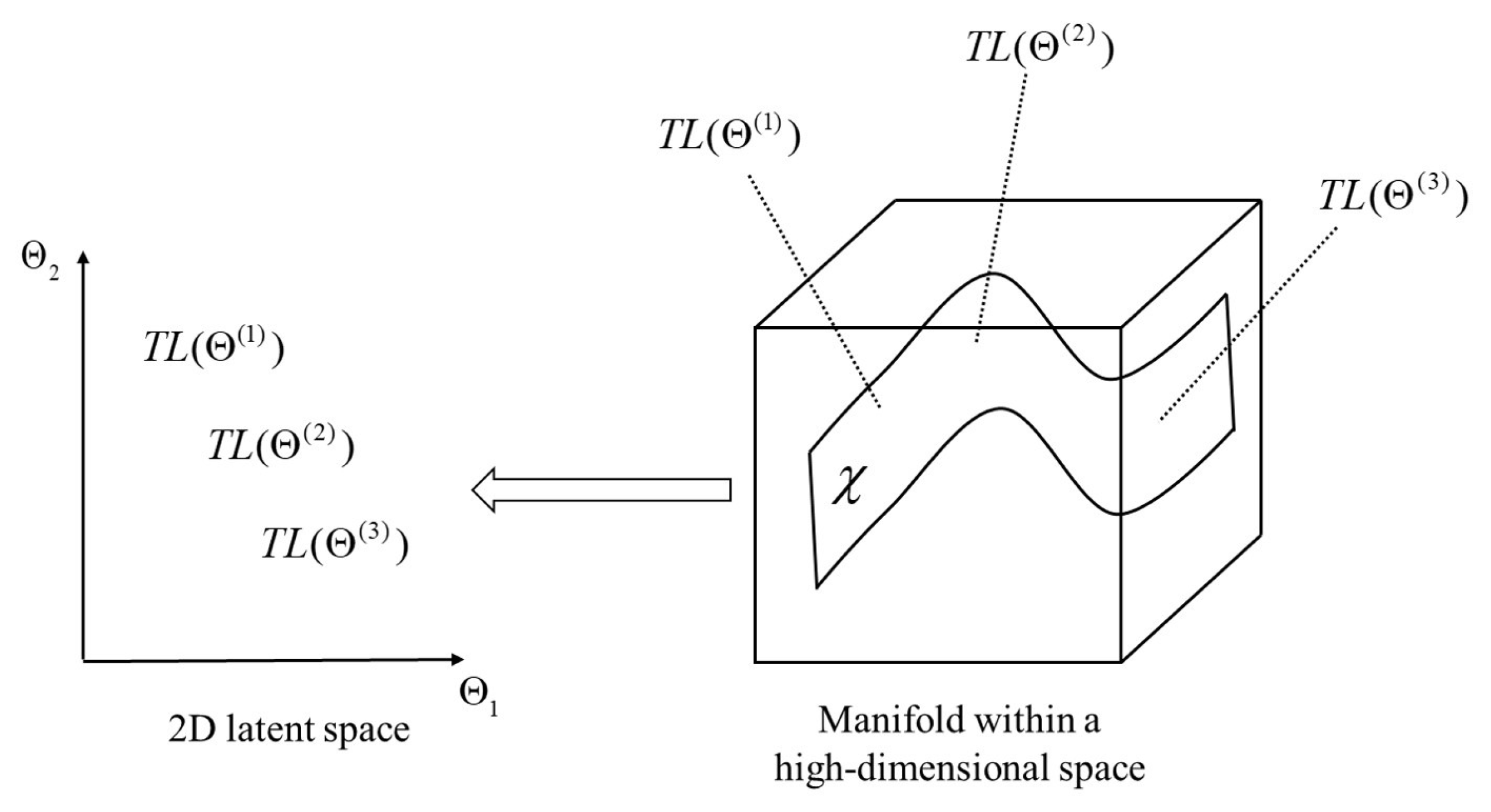
Low-dimensional manifold of TL data
μ Probability measure on manifold M
q ϕ ( z | x ) Encoder/recognition model
p θ ( x | z ) Decoder/generative model
L ( θ , ϕ ) Evidence Lower Bound (ELBO)
D KL Kullback–Leibler divergence
ϵ Random noise variable in reparameterization trick
J Jacobian matrix of transformations
β Decoder output variance hyperparameter

References

  1. Porter, M.B. The Kraken Normal Mode Program; Technical report; Naval Research Laboratory: Washington, DC, USA, 1992. [Google Scholar]
  2. Porter, M.B. Bellhop: A Beam/Ray Trace Code, Version 2010-1. 2010. Available online: https://oalib-acoustics.org/website_resources/AcousticsToolbox/Bellhop-2010-1.pdf (accessed on 7 March 2025).
  3. Kingma, D.P.; Welling, M. Auto-Encoding Variational Bayes. In Proceedings of the 2nd International Conference on Learning Representations, ICLR 2014, Banff, AB, Canada, 14–16 April 2014. [Google Scholar]
  4. Wei, L.; Wang, Z. A Variational Auto-Encoder Model for Underwater Acoustic Channels. In Proceedings of the 15th International Conference on Underwater Networks & Systems (WUWNet ’21), Shenzhen, China, 21–24 November 2021. [Google Scholar]
  5. Goodfellow, I.J.; Pouget-Abadie, J.; Mirza, M.; Xu, B.; Warde-Farley, D.; Ozair, S.; Courville, A.; Bengio, Y. Generative adversarial nets. In Proceedings of the 28th International Conference on Neural Information Processing Systems (NIPS’14), Montreal, QC, Canada, 8–13 December 2014; MIT Press: Cambridge, MA, USA, 2014; Volume 2, pp. 2672–2680. [Google Scholar]
  6. Liu, J.; Zhu, G.; Yin, J. Joint color spectrum and conditional generative adversarial network processing for underwater acoustic source ranging. Appl. Acoust. 2021, 182, 108244. [Google Scholar] [CrossRef]
  7. C., S.C.; Kamal, S.; Mujeeb, A.; M.H., S. Generative adversarial learning for improved data efficiency in underwater target classification. Eng. Sci. Technol. Int. J. 2022, 30, 101043. [Google Scholar] [CrossRef]
  8. Wang, Z.; Liu, L.; Wang, C.; Deng, J.; Zhang, K.; Yang, Y.; Zhou, J. Data Enhancement of Underwater High-Speed Vehicle Echo Signals Based on Improved Generative Adversarial Networks. Electronics 2022, 11, 2310. [Google Scholar] [CrossRef]
  9. Zhou, M.; Wang, J.; Feng, X.; Sun, H.; Li, J.; Kuai, X. On Generative-Adversarial-Network-Based Underwater Acoustic Noise Modeling. IEEE Trans. Veh. Technol. 2021, 70, 9555–9559. [Google Scholar] [CrossRef]
  10. Varon, A.; Mars, J.; Bonnel, J. Approximation of modal wavenumbers and group speeds in an oceanic waveguide using a neural network. JASA Express Lett. 2023, 3, 066003. [Google Scholar] [CrossRef] [PubMed]
  11. Mallik, W.; Jaiman, R.K.; Jelovica, J. Predicting transmission loss in underwater acoustics using convolutional recurrent autoencoder network. J. Acoust. Soc. Am. 2022, 152, 1627–1638. [Google Scholar] [CrossRef]
  12. Sun, Z.; Wang, Y.; Liu, W. End-to-end underwater acoustic transmission loss prediction with adaptive multi-scale dilated network. J. Acoust. Soc. Am. 2025, 157, 382–395. [Google Scholar] [CrossRef] [PubMed]
  13. Jensen, F.B.; Kuperman, W.A.; Porter, M.B.; Schmidt, H. Computational Ocean Acoustics, 2nd ed.; Springer Publishing Company, Incorporated: New York, NY, USA, 2011. [Google Scholar]
  14. Zhang, X.; Wang, P.; Wang, N. Nonlinear dimensionality reduction for the acoustic field measured by a linear sensor array. MATEC Web Conf. 2019, 283, 07009. [Google Scholar] [CrossRef]
  15. Ray, D.; Pinti, O.; Oberai, A.A. Generative Deep Learning. In Deep Learning and Computational Physics; Springer Nature: Cham, Switzerland, 2024; pp. 121–146. [Google Scholar]
  16. Dai, B.; Wipf, D.P. Diagnosing and Enhancing VAE Models. In Proceedings of the 7th International Conference on Learning Representations, ICLR 2019, New Orleans, LA, USA, 6–9 May 2019. [Google Scholar]
  17. Loaiza-Ganem, G.; Ross, B.L.; Cresswell, J.C.; Caterini, A.L. Diagnosing and Fixing Manifold Overfitting in Deep Generative Models. arXiv 2022, arXiv:2204.07172. [Google Scholar]
  18. Loaiza-Ganem, G.; Ross, B.L.; Hosseinzadeh, R.; Caterini, A.L.; Cresswell, J.C. Deep Generative Models through the Lens of the Manifold Hypothesis: A Survey and New Connections. arXiv 2024, arXiv:2404.02954. [Google Scholar]
  19. Rezende, D.J.; Mohamed, S. Variational inference with normalizing flows. In Proceedings of the 32nd International Conference on International Conference on Machine Learning (ICML’15), Lille, France, 6–11 July 2015; Volume 37, pp. 1530–1538. [Google Scholar]
  20. Dinh, L.; Sohl-Dickstein, J.; Bengio, S. Density estimation using Real NVP. In Proceedings of the 5th International Conference on Learning Representations, ICLR 2017, Toulon, France, 24–26 April 2017. [Google Scholar]
  21. Su, J.; Wu, G. f-VAEs: Improve VAEs with Conditional Flows. arXiv 2018, arXiv:1809.05861. [Google Scholar]
  22. He, K.; Zhang, X.; Ren, S.; Sun, J. Deep Residual Learning for Image Recognition. In Proceedings of the 2016 IEEE Conference on Computer Vision and Pattern Recognition (CVPR), Las Vegas, NV, USA, 27–30 June 2016; pp. 770–778. [Google Scholar]
  23. Dinh, L.; Krueger, D.; Bengio, Y. NICE: Non-linear Independent Components Estimation. In Proceedings of the 3rd International Conference on Learning Representations, ICLR 2015, San Diego, CA, USA, 7–9 May 2015. [Google Scholar]
  24. Kingma, D.P.; Dhariwal, P. Glow: Generative Flow with Invertible 1x1 Convolutions. In Proceedings of the Advances in Neural Information Processing Systems 31: Annual Conference on Neural Information Processing Systems 2018, NeurIPS 2018, Montréal, QC, Canada, 3–8 December 2018; pp. 10236–10245. [Google Scholar]
  25. Zhai, S.; Zhang, R.; Nakkiran, P.; Berthelot, D.; Gu, J.; Zheng, H.; Chen, T.; Bautista, M.Á.; Jaitly, N.; Susskind, J.M. Normalizing Flows are Capable Generative Models. arXiv 2024, arXiv:2412.06329. [Google Scholar]
Figure 1. Schematic diagram of a low-dimensional manifold embedded in high-dimensional space.
Jmse 13 01325 g001
Figure 2. Hybrid VAE–Flow framework through two-stage training strategy for underwater acoustic TL prediction.
Jmse 13 01325 g002
Figure 3. Schematic diagram of a shallow-water waveguide with negative thermocline.
Jmse 13 01325 g003
Figure 4. Flowchart for sound speed profile generation via empirical orthogonal decomposition.
Jmse 13 01325 g004
Figure 5. Average sound speed profile and the first two EOF modes. (a) Average SSP. (b) Spatial patterns of the first two EOF modes.
Jmse 13 01325 g005
Figure 6. Schematic diagram of VAE network architecture.
Jmse 13 01325 g006
Figure 7. Schematic diagram of Flow network architecture.
Jmse 13 01325 g007
Figure 8. Training and validation curves of the VAE network. (a) Reconstruction loss. (b) KL loss.
Jmse 13 01325 g008
Figure 9. Comparison between the TL results of the KRAKEN and the VAE network under different test EOF coefficients.
Jmse 13 01325 g009
Figure 10. SSIM of acoustic TL fields reconstructed by the VAE network against KRAKEN simulations on the training and test sets.
Jmse 13 01325 g010
Figure 11. Comparison between distributions in 2D space. (a) Latent variables. (b) EOF coefficients.
Jmse 13 01325 g011
Figure 12. Training and validation curves of the Flow network.
Jmse 13 01325 g012
Figure 13. The probability density of the fitted distributions against the ground truth. (a) Flow fitting results in Dimension 1. (b) Flow fitting results in Dimension 2. (c) Simplified VAE fitting results in Dimension 1. (d) Simplified VAE fitting results in Dimension 2.
Jmse 13 01325 g013
Figure 14. Comparison of performance between Flow network and simplified VAE network on MSE. (a) The first dimension. (b) The second dimension.
Jmse 13 01325 g014
Figure 15. Comparison between the TL results of the KRAKEN and the VAE–Flow network under different EOF test coefficients.
Jmse 13 01325 g015
Figure 16. SSIM of acoustic TL fields reconstructed by the VAE network against KRAKEN simulations, and predicted by the VAE–Flow network against KRAKEN simulations on distinct datasets. (a) Reconstructed SSIM results on D1–D6. (b) Predicted SSIM results on D1–D6. (c) Reconstructed SSIM results between original and augmented D6. (d) Predicted SSIM results between original and augmented D6.
Jmse 13 01325 g016
Figure 17. Comparison of the computational time of the VAE–Flow network and KRAKEN model.
Jmse 13 01325 g017
Table 1. Sampling distribution of the six datasets.
Dataset a 1 N ( μ 1 , σ 1 2 ) a 2 N ( μ 2 , σ 2 2 )
D1 μ 1 = 0 , σ 1 = 0.5 μ 2 = 0 , σ 2 = 0.25
D2 μ 1 = 0 , σ 1 = 1.0 μ 2 = 0 , σ 2 = 0.5
D3 μ 1 = 0 , σ 1 = 1.0 μ 2 = 0 , σ 2 = 1.0
D4 μ 1 = 0 , σ 1 = 2.0 μ 2 = 0 , σ 2 = 1.0
D5 μ 1 = 0 , σ 1 = 3.0 μ 2 = 0 , σ 2 = 3.0
D6 μ 1 = 0 , σ 1 = 10.0 μ 2 = 0 , σ 2 = 5.0
Disclaimer/Publisher’s Note: The statements, opinions and data contained in all publications are solely those of the individual author(s) and contributor(s) and not of MDPI and/or the editor(s). MDPI and/or the editor(s) disclaim responsibility for any injury to people or property resulting from any ideas, methods, instructions or products referred to in the content.

