A Ship Underwater Radiated Noise Prediction Method Based on Semi-Supervised Ensemble Learning

Abstract

Accurate prediction of ship underwater radiated noise (URN) during navigation is critical for evaluating acoustic stealth performance and analyzing detection risks. However, the labeled data available for the training of URN prediction model is limited. Semi-supervised learning (SSL) can improve the model performance by using unlabeled data in the case of a lack of labeled data. Therefore, this paper proposes an SSL method for URN prediction. First, an anti-perturbation regularization is constructed using unlabeled data to optimize the objective function of EL, which is then used in the Genetic algorithm to adaptively optimize base learner weights, to enhance pseudo-label quality. Second, a semi-supervised ensemble (ESS) framework integrating dynamic pseudo-label screening and uncertainty bias correction (UBC) is established, which can dynamically select pseudo-labels based on local prediction performance improvement and reduce the influence of pseudo-labels’ uncertainty on the model. Experimental results of the cabin model and sea trials of the ship demonstrate that the proposed method reduces prediction errors by up to 65.5% and 62.1% compared to baseline supervised and semi-supervised regression models, significantly improving prediction accuracy.

1. Introduction

Underwater Radiation Noise (URN) serves as a critical information source for enemy detection [1]. Real-time monitoring of a vessel’s acoustic status is essential to scientifically implement vibration and noise reduction measures and enhance stealth capabilities [2]. Accurate prediction of URN is pivotal for acoustic state monitoring. During vessel navigation, machinery systems, propellers, and fluid action can generate three principal noise components: mechanical noise, propeller noise, and hydrodynamic noise [3,4]. These propagate through seawater and collectively constitute URN in the far field.

Scholars have developed various approaches to predict the ship URN. For simple structures such as plates, elastic spherical shells, and cylindrical shells [5,6,7,8], analytical methods are proposed to assess vibration-induced acoustic radiation. For complex ship structures, semi-analytical/numerical hybrid methods [9,10,11,12,13] are typically employed, focusing on structural or propeller noise prediction during the design phase. In engineering applications, semi-theoretical/experimental approaches [14,15,16,17] are widely adopted for URN prediction. It is a common practice that transfer functions between hull vibrations and radiated noise are established using data from cale-model simulations or vibration-acoustic experiments. Esen Cintosun [15] proposed two empirical methods, AQV (Acceleration-based Quantitative Velocity) and NNLS (Non-Negative Least Squares), which construct transfer functions from vibration-acceleration measurements to estimate underwater noise. Compared to traditional volume, velocity, and equivalent radiated power methods, NNLS demonstrated superior full-frequency prediction accuracy. Linchang Ye [16] addressed the ill-posed transfer function estimation caused by limited experimental data by using the regularization of the total least squares. A Peak-based Gated Recurrent Unit (PGRU) neural network was integrated to correct prediction errors, enhancing noise reconstruction accuracy. Uyeup Park [17] combined neural networks with operational transfer path analysis (OTPA), circumventing underdetermined equations in transfer function inversion while preserving critical acoustic information.

In recent years, machine learning (ML) and artificial intelligence methodologies have been increasingly applied to ship URN evaluation [18,19,20,21], with techniques such as Support Vector Machines (SVM), Radial Basis Function (RBF) Neural Networks, and Deep Neural Networks (DNN), et al. However, current ML methods for URN prediction predominantly rely on simulated training data [22]. This practice faces two critical limitations. Firstly, numerical simulations struggle to authentically replicate the complex marine hydrodynamic environments during underwater navigation. Secondly, simulation models lack sufficient fidelity for researching intricate underwater structures, particularly geometrically complex ship structures. These factors significantly compromise the reliability of synthetic datasets.

More trustworthy data must be derived from vibration-acoustic measurements during actual sea trials, necessitating dedicated ship noise experiments. Nevertheless, vibration-acoustic experiments remain cost-prohibitive [23], with high expenses associated with large-scale labeled data acquisition. Furthermore, operational constraints during radiated noise measurements limit the diversity of experimental conditions. Consequently, most obtainable training samples consist solely of hull vibration measurements (unlabeled data), while paired radiated noise observations (labeled data) constitute only a small fraction of the dataset.

To address the scarcity of labeled data in ship URN prediction, semi-supervised learning (SSL) provides a viable solution by jointly leveraging limited labeled data and abundant unlabeled data, thereby reducing the heavy reliance on annotated data in traditional supervised regression [24]. SSL operates under foundational assumptions including the cluster assumption, smoothness assumption, and manifold assumption [25]. These principles enable SSL to utilize the distributional patterns of unlabeled data to enhance learning from labeled samples while improving generalization capabilities [26]. SSL encompasses two primary paradigms, which are semi-supervised classification (SSC) and semi-supervised regression (SSR). While SSC has achieved widespread adoption in domains such as natural language processing (NLP), image recognition, and semantic segmentation [27,28,29], SSR remains understudied in engineering applications [30]. The common SSL methods include generative models, semi-supervised kernel regression, graph-based approaches, and disagreement-based SSL. Among these, disagreement-based methods are more widely applied, including self-raining (ST) [31], co-training (CT) [32,33], and tri-training (TT) [34,35].

Subsequent extensions of TT laid the foundation for early semi-supervised ensemble (ESS) frameworks, exemplified by the Co-Forest (CF) algorithm. SSL and ensemble learning (EL) represent two pivotal ML paradigms. Through their synergistic integration, SSL enriches EL with augmented training samples via pseudo-labeling, while EL enhances SSL by supplying diverse base learners. Theoretical studies demonstrate that this combination yields models with superior generalization capabilities [36]. To address the dual challenges of limited labeled data and suboptimal model generalization in ship URN prediction, this work adopts an ESS framework. The core research focus lies in effectively harmonizing SSL and EL to enhance pseudo-label quality while mitigating noise contamination from low-confidence pseudo-labels, which could degrade model performance.

To address these challenges, this paper proposes an UBC-AWESSR model, which has better performance and fast prediction speed. The main contributions of this paper are summarized as follows:

(1)

A genetic algorithm-based adaptive weighted ensemble (AWE) model is proposed. By constructing an anti-perturbation regularization term using unlabeled data, this framework optimizes base learner weights to enhance pseudo-label quality while improving ensemble robustness.

(2)

An ensemble semi-supervised regression (ESSR) model integrating dynamic pseudo-label screening and uncertainty bias correction (UBC) is established. Pseudo-labels are dynamically filtered based on local prediction performance improvement. Ensemble prediction variance quantifies pseudo-label uncertainty, with sample weights assigned via uncertainty-aware adjustment to minimize bias in training.

(3)

The UBC-AWESSR method proposed in this study is validated by cabin model experiments and sea trials of the vessel. Results confirm its superior performance in static and dynamic scenarios, outperforming traditional supervised regression (SR) and semi-supervised regression (SSR) models with maximum error reductions of 65.5% and 62.1%, respectively.

The remainder of this paper is organized as follows. Section 2 reviews related work. Section 3 details the research problem, methodology, and the overall framework of the ship URN prediction model. Section 4 validates the effectiveness of the proposed method. Finally, Section 5 summarizes the key conclusions.

2. Related Work

2.1. Consistency Regularization

Consistency Regularization (CR) serves as a pivotal SSL method that leverages unlabeled data to enhance feature extraction without label dependency, delivering robust performance under limited labeled data. Among CR methods, Virtual Adversarial Training (VAT) was introduced by Miyato et al. (2018) [37], defining adversarial perturbation directions based on the smoothness assumption. VAT computes the gradient of model predictions relative to input perturbations to generate maximally disruptive adversarial samples, enforcing output consistency between original and perturbed inputs, thereby improving model generalization.

In ship URN prediction, VAT can generate perturbations to simulate sensor-introduced external interference, improving the model’s alignment with physical mechanisms. Unlike traditional methods such as Temporal Ensembling [38], which merely suppresses noise through temporal averaging and lacks physical interpretability, our approach leverages VAT to identify adversarial perturbation directions most sensitive to sample data. By integrating acoustics-specific contexts, this strategy enforces stronger local smoothness constraints, thereby enhancing model performance.

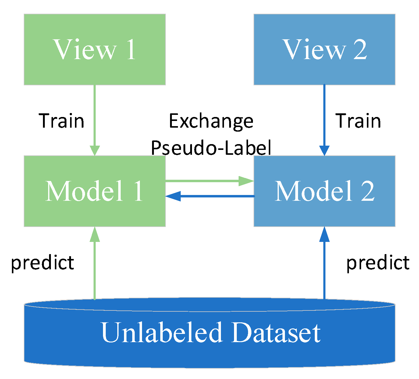
2.2. Semi-Supervised Co-Training Based on Disagreement

Semi-supervised co-training exploits inter-learner disagreement [39] under the multi-view assumption, which posits that data can be represented by multiple distinct feature spaces. This framework leverages complementary information from distinct views for the target task, iteratively assigning high-confidence pseudo-labels to unlabeled data for self-augmentation and cooperative optimization, as illustrated in Figure 1. However, the multi-view assumption is often restrictive—most real-world datasets only possess a single attribute set, making it challenging to partition mutually redundant views. Consequently, co-training variants have emerged, achieving disagreement maximization by exploiting discrepancies among multiple learners within a single view. Building on this principle, our method harnesses the intrinsic model diversity of ensemble learning to maximize disagreement.

2.3. Ensemble Semi-Supervised Learning

Inspired by disagreement-based SSL, ensemble semi-supervised (ESS) learning has been developed. This framework integrates ensemble strategies with semi-supervised mechanisms, achieving “disagreement maximization” through collaborative optimization of diverse base learners, thereby fully leveraging the latent information from limited labeled data and abundant unlabeled data to enhance model predictive performance. ESS has been widely adopted in classification tasks. A representative example is tri-training (TT), an ESS classification model that employs three classifiers to bypass direct confidence estimation of predictions. Instead, it uses the “majority voting” principle to select high-confidence pseudo-labels [34]. In SSL, classification tasks can directly quantify the prediction confidence of unlabeled samples via base classifiers’ posterior probabilities. However, regression tasks face a core challenge; their continuous outputs lack probabilistic representations, complicating the evaluation of pseudo-label confidence for effective screening. To address this, we propose a novel ESS model based on dynamic pseudo-label screening and UBC. By coordinating multiple regressors, this approach improves pseudo-label quality while reducing uncertainties in pseudo-labels used for model training.

3. Methodology

3.1. Symbol Setting

This study aims to address the problem of the ship URN prediction. We define labeled data 𝓛 as the dataset obtained from ship noise measurement trials, which includes hull vibration data and the corresponding radiated noise data, expressed as follows.

$$\text{𝓛}=\left\{\left(x_l{}^1,{y_l}^1\right),\left(x_l{}^2,{y_l}^2\right),\cdots ,\left(x_l{}^{\left|n_l\right|},{y_l}^{\left|n_l\right|}\right)\right\}$$

(1)

The unlabeled data 𝓤 consists of vibration data collected during navigation, as shown in Equation (2).

$$\text{𝓤}=\left\{x_u{}^1,x_u{}^2,\cdots ,{x_u}^{\left|n_u\right|}\right\}$$

(2)

In Equations (1) and (2), each input sample $x_i\in {ℝ}^d$ represents hull vibration data, where the dimensionality d is equal to the number of vibration monitoring sensors. The variable $y_i\in ℝ$ is the actual measured URN. $\left|n_l\right|$ and $\left|n_u\right|$ denote the number of labeled and unlabeled samples, respectively. The prediction model is trained on the combined dataset 𝓓 = 𝓛 $\cup$ 𝓤 to learn a regression function $f:{ℝ}^d\to ℝ$, trying to minimize the prediction error on a testing sample. Notably, the data during collecting may contain random perturbations from external factors, posing challenges to the model’s generalization capability and robustness.

3.2. Adaptive Weighted Ensemble (AWE) Learning Based on Genetic Algorithm

3.2.1. Objective Function Optimization

The EL model serves as the core component of the ESS learning framework, functioning to predict pseudo-labels for unlabeled data during training. We have researched the details of the EL model in [40], and the selection of the base model for the EL and the integration method in this paper are based on the research results from [40]. The difference is that we improved the objective function here based on the principle of consistency regularization introduced in Section 2.1. The improved objective function introduces an anti-perturbation regularization term using unlabeled data to effectively improve the data utilization rate. On the other hand, the difference in model estimates before and after perturbation can be used to constrain model training, which is conducive to improving the model robustness.

This work employs VAT to design an anti-perturbation regularization term for the EL model’s objective function. This term quantifies the prediction discrepancy between perturbed and original unlabeled samples, operates without actual labels, and effectively leverages unlabeled data for model training, which can mitigate error propagation caused by incorrect pseudo-label assignments.

$\widehat{y}=h\left(x\right)$ represents the prediction result of model h for the input x. Considering the influence of data perturbation, $x+\xi$ represents the input after adding disturbances, $\xi$ represents a specific directional disturbance to x.

$${\widehat{y}}_d=h\left(x+\xi \right)$$

(3)

Here, ${\widehat{y}}_d$ is the output result of the model under the condition that the input x is disturbed.

$L_{semi}$ is the optimized objective function for ESS learning, $L\left({\widehat{y}}_i,y_i\right)$ is the deviation between the output of the model ${\widehat{y}}_i$ and the true value $y_i$ when the input is $x_i$, $L_{CR}\left({\widehat{y}}_i{}^u,{{\widehat{y}}_{di}}^u\right)$ is the anti-perturbation regularization loss of unlabeled data, and ${{\widehat{y}}_i}^u$ and ${{\widehat{y}}_{di}}^u$ are outputs of the unlabeled samples ${x_i}^u$ before and after adding disturbances. $L$ and $L_{CR}$ are all measured by the root mean square error (RMSE). In this paper, the objective function is defined as the supervised loss on labeled datasets and the unsupervised regularization loss on unlabeled datasets, as follows:

$$L_{semi}={\displaystyle \frac{1}{\left|n_l\right|}}{\displaystyle \sum _{i=1}^{\left|n_l\right|}L\left({\widehat{y}}_i{}^l,{y_i}^l\right)}+{\displaystyle \frac{\lambda }{\left|n_u\right|}}{\displaystyle \sum _{i=1}^{\left|n_u\right|}{L}_{CR}\left({\widehat{y}}_i{}^u,{{\widehat{y}}_{di}}^u\right)}$$

(4)

where ${\displaystyle \frac{\lambda }{\left|n_u\right|}}{\displaystyle \sum _{i=1}^{\left|n_u\right|}{L}_{CR}\left({\widehat{y}}_i{}^u,{{\widehat{y}}_{di}}^u\right)}$ is an unsupervised regularization term and $\lambda$ is the regularization coefficient.

3.2.2. Adaptive Weighting

The advantage of EL lies in integrating multiple models and leveraging the diversity of models to enhance the performance of SSL. The adaptive weighting of the base learners can dynamically search for the optimal weight distribution through genetic operations, solve the limitations of the traditional static weighting method under complex data distribution, and effectively improve the performance of the prediction model.

Suppose there are M base learners, the output is ${\left\{f_m\right\}}_{m=1}^M$, the weight of each base learner is $w_m$, and the prediction result of the EL model is

$${\widehat{y}}_{EM}\left(x\right)={\displaystyle \sum _{m=1}^M{w}_m{f}_m\left(x\right)}$$

(5)

where $w_m\in \left[0,1\right]$ and ${\displaystyle \sum _{m=1}^M{w}_m}=1$.

In this paper, the training objective of EL is to minimize the prediction error of the validation set while keeping the anti-perturbation regularization term as small as possible. However, genetic algorithms tend to select individuals with higher fitness. Therefore, combined with the optimized objective function in the previous section, the fitness function is defined as follows:

$$Fitness\left(\mathit{w}\right)={\displaystyle \frac{1}{1+L_{semi}\left(\mathit{w}\right)}}$$

(6)

The weight vector $\mathit{w}=\left[w_1,w_2,\cdots ,w_M\right]$ is encoded as a chromosome in real numbers. The weights are forced to be satisfied ${\displaystyle \sum _{m=1}^M{w}_m}=1$ through a softmax normalization transformation, and the transformation process is as follows:

$$w_m={\displaystyle \frac{\exp \left(z_m\right)}{{\displaystyle \sum _{m=1}^M\exp \left(z_m\right)}}}$$

(7)

where $z_m$ is the variable to be optimized. Firstly, initialize the chromosome code and calculate the fitness function value of the current individual. Select the excellent individuals with higher fitness values as the parent generation. Then, through cross-operation and mutation operation, obtain the next generation population, and calculate the fitness value. Subsequently, perform a cyclic operation. Through continuous iterative optimization, the optimal solution output of the weight is finally obtained to achieve the adaptive weighting of the EL model.

3.3. ESS Based on Pseudo-Label Dynamic Screening and Uncertainty Bias Correction

Labeled data trains a supervised model to generate pseudo-labels for unlabeled samples, thereby expanding the training dataset. However, pseudo-label suffers from confirmation bias, where initial model errors propagate and amplify through iterative pseudo-label injection, leading to performance degradation. To mitigate this issue, we integrate a dynamic pseudo-label selection mechanism with UBC. This method screens pseudo-labels based on their contribution to local prediction improvements and quantifies uncertainty using ensemble variance, significantly enhancing the quality of pseudo-labels used in training.

3.3.1. Dynamic Screening of Pseudo-Labels

In SSR, pseudo-label screening is a key link to improve the generalization ability of the model. This paper does not set a specific confidence threshold. Instead, the reliability of pseudo-labels is evaluated by the change in the model’s prediction performance after adding unlabeled data, thereby screening out the pseudo-labels that are beneficial to the improvement of the model’s performance.

For each unlabeled sample $x_u$, the evaluation index of its predicted value is assessed by quantifying its impact on the labeled dataset. The expression for the evaluation indicators $\Delta x_u$ is as follows:

$$\Delta x_u={\displaystyle \sum _{x_i\in \Phi }\left[{\left(y_i-h\left(x_i\right)\right)}^2-{\left(y_i-h^{\prime }\left(x_i\right)\right)}^2\right]}$$

(8)

Among them, h is the original regressor, h’ is the updated regressor after fusion $\left(x_u,{\widehat{y}}_u\right)$. $\Phi$ represents the subset of the k-nearest neighbor (KNN) supervised samples of $x_u$. The local consistency test is achieved by calculating the sum of the predicted residuals of the KNN supervised samples. The pseudo-label samples corresponding to $\Delta x_u>0$ are screened out, which are the pseudo-label samples that improve the performance of the model. Selecting the KNN labeled sample of $x_u$ from the labeled data for confidence analysis can reduce the number of target samples and improve the training efficiency of the model.

3.3.2. Uncertainty Bias Correction

The bias correction mechanism aims to solve the confirmation bias problem introduced by the pseudo-labels of unlabeled data. In this paper, the variance is calculated based on the prediction results of the EL base learners to correct the uncertainty bias of pseudo-labels. The larger the variance, the greater the uncertainty of the pseudo-label and the lower the confidence. The pseudo-labels of such high-variance samples are assigned lower weights to reduce the interference of uncertainty on model training, while for the low-variance samples, their contributions will be enhanced.

According to the EL model in Section 3.2.2, which is adaptively weighted, the outputs of different base learners can be expressed as

$${f_m}^{\prime }\left(x\right)=w_m{f}_m\left(x\right)$$

(9)

The variance of the prediction results of different base learners is

$${\sigma }^2={\displaystyle \frac{1}{M}}{{\displaystyle \sum _{m=1}^M\left({f_m}^{\prime }\left(x\right)-\mu \right)}}^2$$

(10)

$\mu ={\displaystyle \frac{1}{M}}{\displaystyle \sum _{m=1}^M{f_m}^{\prime }\left(x\right)}$ is the mean of the prediction results of the base learners.

This paper adopts the exponential decay weighting method and defines the sample weights as

$$W=e^{-\beta \cdot {\sigma }^2}$$

(11)

where $\beta$ > 0 is used to control the speed of weight attenuation. To improve the quality of pseudo-labels, the objective function designed in Section 3.2.1 is optimized further, incorporating the uncertainty weights into the training objective. The updated objective function is shown as Equation (12).

$${L_{semi}}^{\prime }={\displaystyle \frac{1}{\left|n_l\right|}}{\displaystyle \sum _{i=1}^{\left|n_l\right|}{W}_i\cdot L\left({\widehat{y}}_i{}^l,{y_i}^l\right)}+{\displaystyle \frac{\lambda }{\left|n_u\right|}}{\displaystyle \sum _{i=1}^{\left|n_u\right|}{L}_{CR}\left({\widehat{y}}_i{}^u,{{\widehat{y}}_{di}}^u\right)}$$

(12)

Based on the above research content, the pseudo-label samples and their training weights for the final training were screened out. The pseudo-code is shown in Algorithm 1.

Algorithm 1. Pseudo-code of UBC-AWESSR model pseudo-label screening

Input: Labeled dataset: 𝓛;             Unlabeled dataset: 𝓤;             Trained ensemble models (EMs): {f1, f2, ..., fM}             Maximum number of learning iterations: T

Output: Get pseudo-label dataset 𝓤_pseudo: {(xu, ŷu, Wu)}

Initialize 𝓤_pseudo = [ ] Repeat for T rounds:      𝓤’ is randomly selected from 𝓤, the size of 𝓤’ is s, the remaining part of 𝓤 is 𝓤0

for xu ∈ 𝓤’ do

Φ ← KNN(xu, 𝓛)            h ← EMs(𝓛, 𝓤0)

$\begin{array}{ll}& {\hat{y}}_u,W_u\leftarrow h\left(x_u\right)\\ & h^{\prime }\leftarrow \mathrm{E}\mathrm{M}\mathrm{s}\left(\mathcal{L}\cup \left\{\left(x_u,{\hat{y}}_u\right)\right\},{\mathcal{U}}_0\right)\end{array}$

$\mathsf{\Delta }{x}_u\leftarrow {\displaystyle \sum _{x_i\in \mathsf{\Phi }}}\left({\left(y_i-h\left(x_i\right)\right)}^2-{\left(y_i-h^{\prime }\left(x_i\right)\right)}^2\right)$

end      If exist $\Delta x_u>0$           $x_u\leftarrow \arg \max \mathsf{\Delta }{x}_u,{\widehat{y}}_u,W_u\leftarrow h\left(x_u\right)$           𝓤_pseudo ← $\left\{\left(x_u,{\widehat{y}}_u,W_u\right)\right\}$

h ← EMs(𝓛 ∪ 𝓤_pseudo, 𝓤0)           𝓤’← 𝓤’ remove $x_u$           𝓤 ← 𝓤’      Else           𝓤_pseudo ← $\varnothing$      End End the repeat

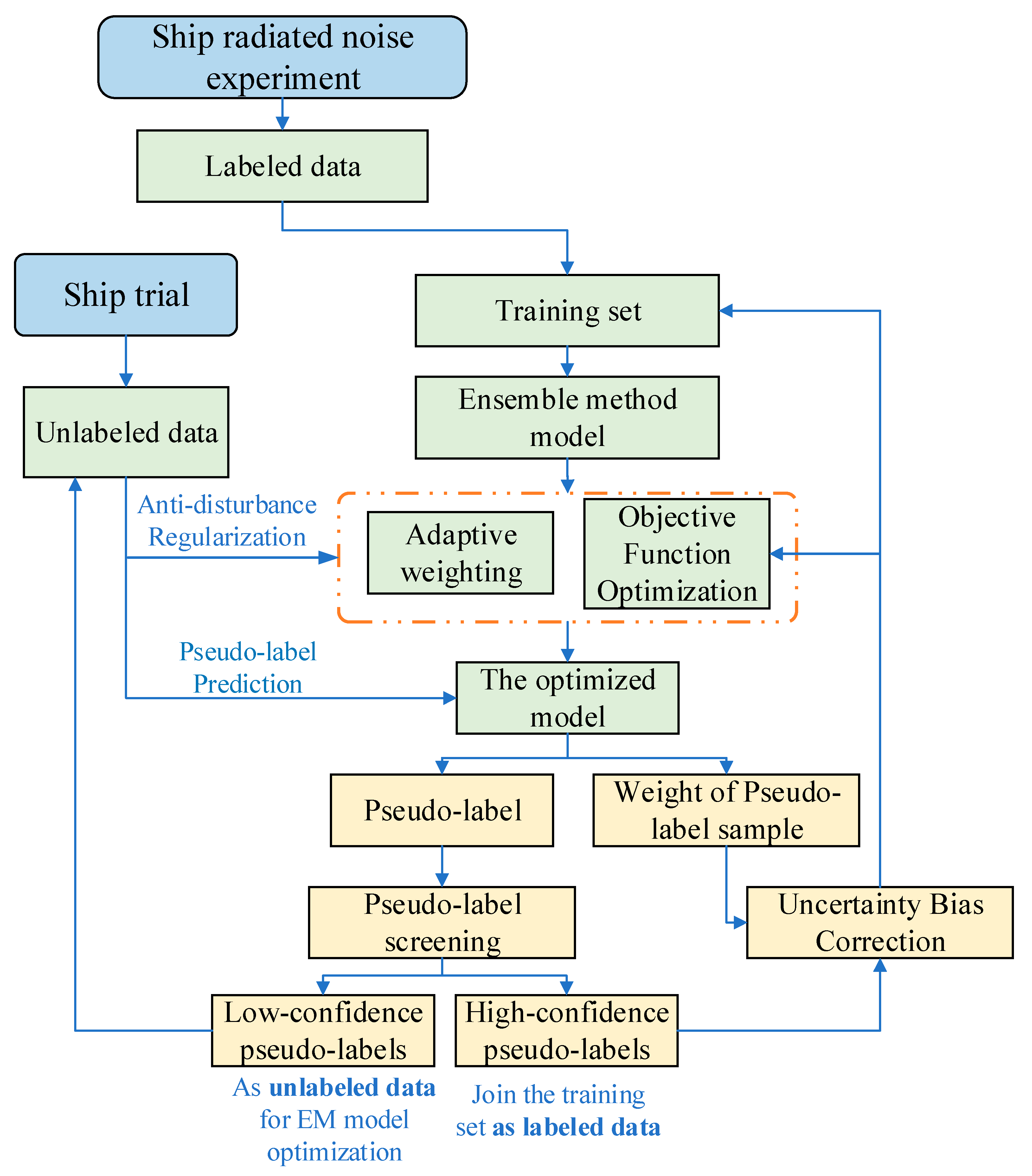
3.4. The Overall Framework of the Ship URN Prediction Model

Based on the ESS model, this paper makes full use of the unlabeled data from two aspects. On the one hand, an anti-perturbation regularization term is added to the objective function of the EL model to implicitly use the unlabeled data. On the other hand, the pseudo-label samples obtained by the EL model are utilized to expand the training dataset, which achieves the optimal utilization of the data. Figure 2 shows the overall framework of the ship URN prediction model based on ESS learning proposed in this paper. The modeling process mainly includes the following steps.

(1)

Multi-source data acquisition and preprocessing

The multi-source data used in this study mainly refer to the acceleration sensor data for monitoring the vibration of the ship and the hydrophone data for monitoring the radiated noise of the ship. The label dataset 𝓛 $={\left\{\left(x_l{}^i,{y_l}^i\right)\right\}}_{i=1}^{\left|n_l\right|}$ including ship vibration data and noise data were established by the ship URN test experiment. A large amount of ship vibration data collected during navigation constitutes the unlabeled dataset 𝓤 $={\left\{{x_u}^i\right\}}_{i=1}^{\left|n_u\right|}$. The original data collected in the experiment were all time domain signals. Through preprocessing such as the Fourier transform, the 1/3 octave band level of the frequency domain was obtained as the input feature vector.

(2)

EL model optimization training

Based on the anti-perturbation regularization method, the weights of the base learners are optimized to achieve the collaborative training of labeled and unlabeled data.

(3)

Pseudo-label screening and application

The unlabeled data is labeled using the EL model, and high-confidence pseudo-labels are dynamically screened and injected for supervised enhancement after uncertainty bias correction. The low-confidence data is still regarded as unlabeled data and used with the labeled data in step (2), until all unlabeled data participate in the training or reach the maximum number of training iterations.

4. Experiment

4.1. Introduction of the Dataset

Vibration sound radiation experiments can generally be divided into static experiments and dynamic experiments. Static experiments are mainly used to evaluate the mechanical noise generated by the operation of shipborne mechanical equipment. Dynamic experiments are carried out during the navigation of a ship, and the experiment environment and the URN components of the ship are more complex. There are not only mechanical noises, but also propeller noise and flow noise brought by the ship’s navigation. The components of URN of ships vary at different speeds. At low speeds, mechanical noise accounts for a relatively large proportion, while at medium and high speeds, the proportions of propeller noise and flow noise increase. This paper conducts the vibration acoustic radiation experiment of a cabin model to simulate the static experiment of a ship and takes a scientific research vessel as the test object to carry out the dynamic experiment at sea, respectively, to verify the applicability of the URN prediction method proposed in this paper in two different experiment scenarios.

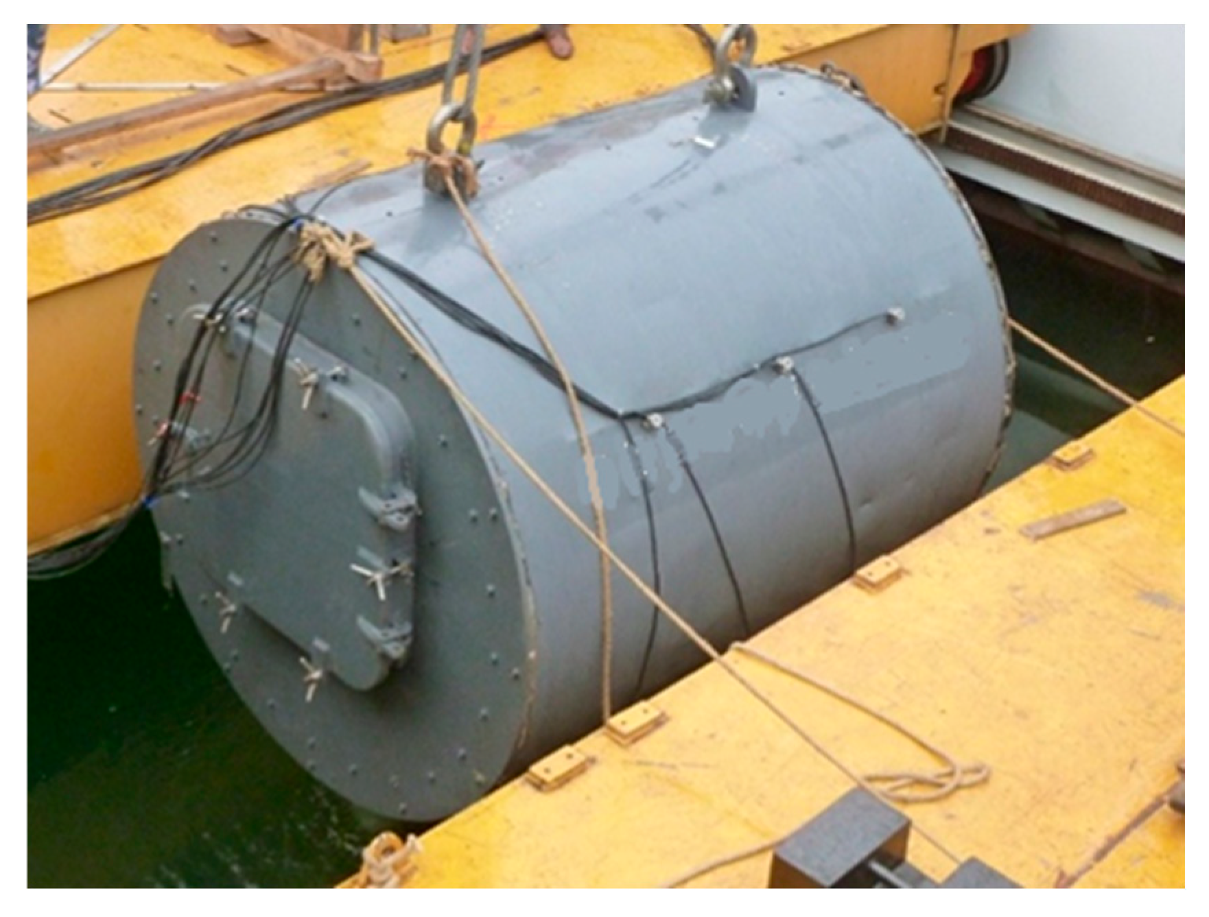
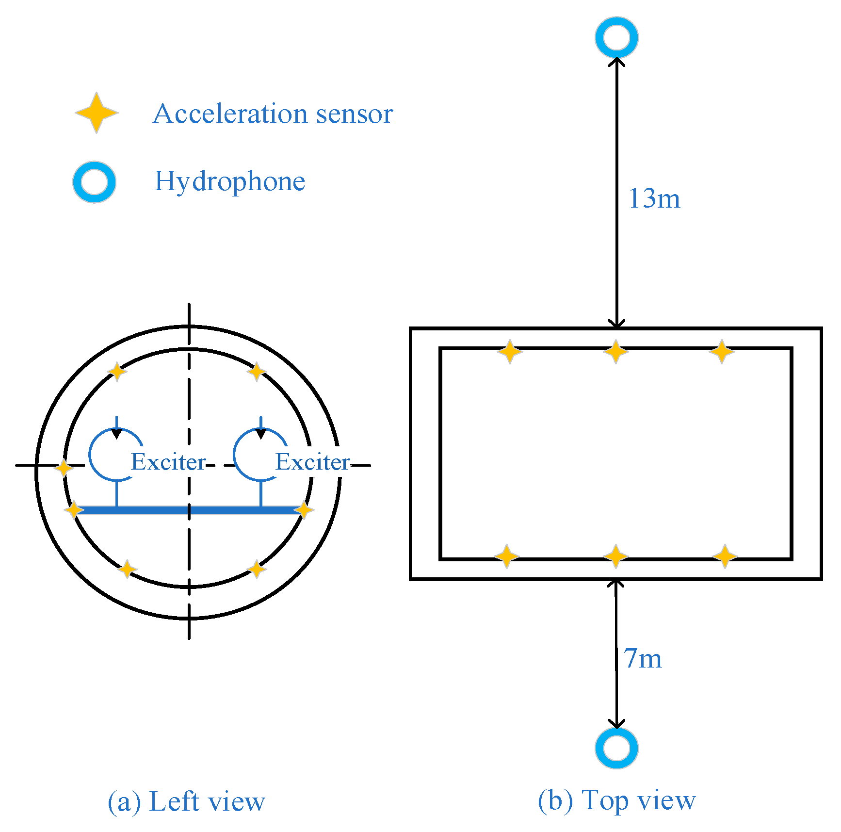
4.1.1. Experiment of the Cabin Model

The cabin model is a double-layer cylindrical shell structure with an outer diameter of 1.78 m, inner diameter of 1.54 m, and length of 2 m, shown as Figure 3. Four exciters are installed inside the cabin, two on the port and starboard sides, respectively, and activated individually to simulate machinery operation scenarios during navigation. The experiment was conducted in water exceeding 50 m depth, with the cabin submerged to a depth of 25 m. Vibration monitoring employed 22 uniformly distributed accelerometers on the inner shell surface, while two hydrophones positioned externally synchronously acquired far-field radiated noise. Figure 4 shows the sensors layout diagram. Here we used BK4514 accelerometer (Brüel & Kjær, Nærum, Denmark) and RESON TC 4032 hydrophone (Reson A/S, Slangerup, Denmark). For accelerometer, the sensitivity is 10 mV/(m·s⁻²), the frequency range is 0.3–10 kHz. For hydrophone, the sensitivity is −170 dB re 1 V/μPa, the frequency range is 5–120 kHz. Before the experiment, all accelerometers and hydrophones were calibrated to ensure measurement accuracy.

Vibration signals collected from machinery mounting points during ship navigation were used as excitation signals for the exciters. By inputting different excitation signals, we simulated actual navigation conditions, resulting in 90 conditions. Each condition data included vibration data from the cabin’s hull and the corresponding URN. The URN served as the output variable, with 22 vibration sensor readings as input features. From the 90 conditions, randomly selected subsets were designated as the test dataset, while the remaining cases were assigned to the training dataset.

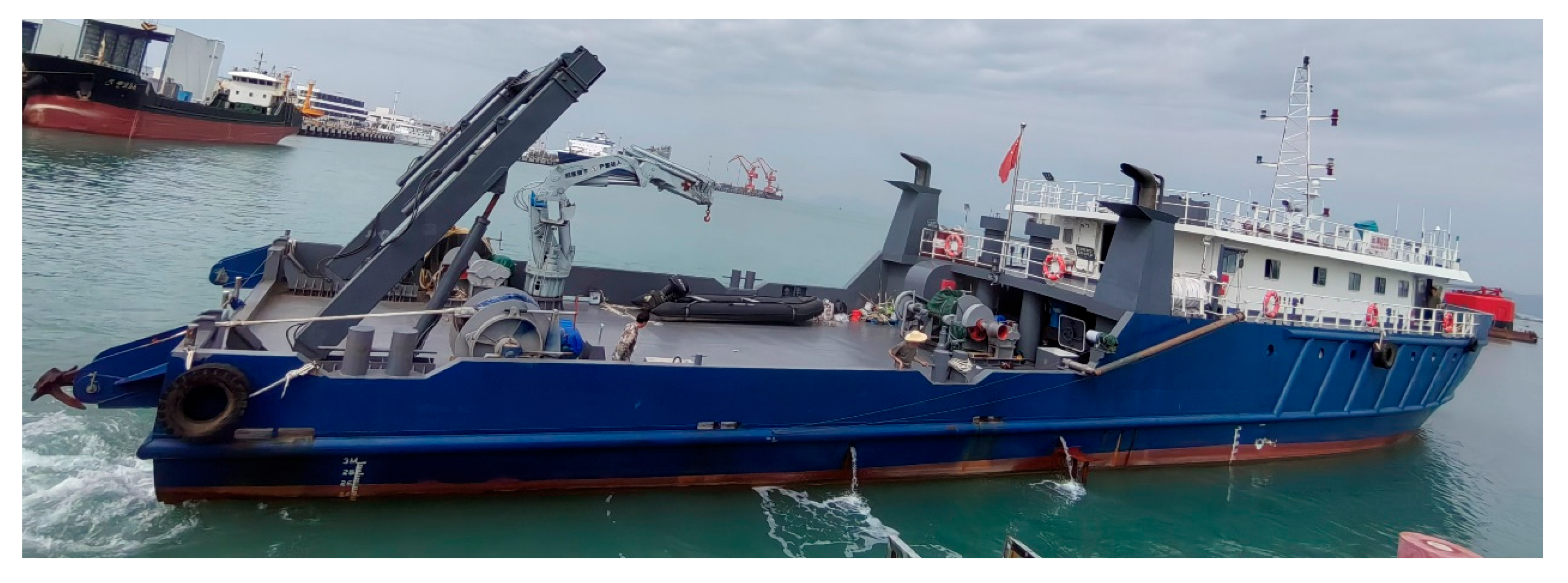
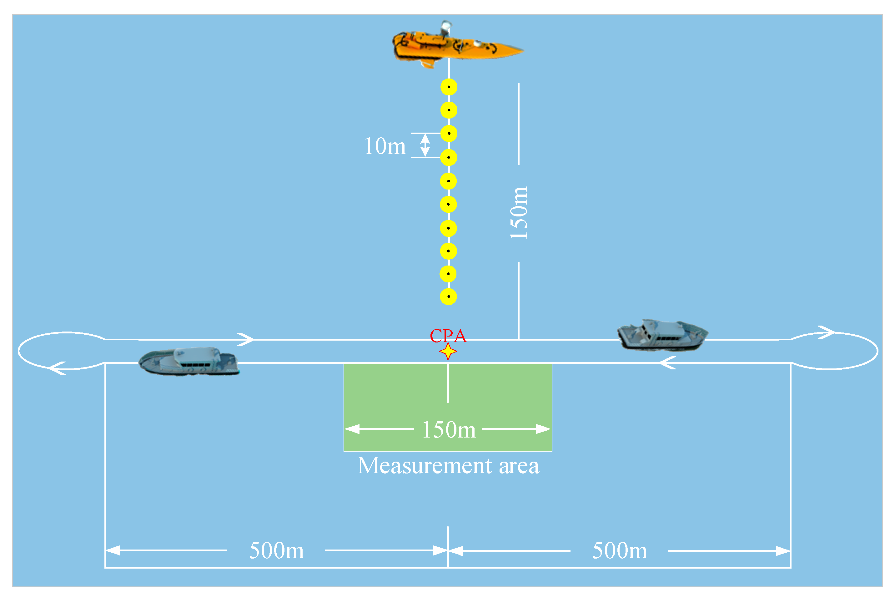
4.1.2. Experiment of the Scientific Research Vessel at Sea

The sea trial was conducted in the South China Sea using a 1000-t scientific research vessel, shown as Figure 5, equipped with a twin-engine dual-propeller system and a maximum speed of 14 knots. Fifty-one vibration accelerometers were installed on machinery mounting points and adjacent ribs to collect vibration data from onboard equipment and the hull. During the experiment, the vessel followed predetermined conditions within a designated area, and a support ship positioned at far-field maintained URN measurement. The accelerometers and hydrophones used in the sea experiment of the research vessel are consistent with the sensors in cabin model experiment.

The schematic diagram of URN measurement at sea is shown in Figure 6. Bule vessel is a research vessel whose URN is measured, and two vessels represent different courses. Yellow ship is an auxiliary ship for URN Measurement. A horizontal hydrophone array is used to measure URN from the research vessel, shown as the yellow dots in Figure 6. Through multi-position synchronous measurement, it can help to eliminate the influence of the sound propagation path and perform distance normalization, also it is easier to deploy compared to vertical arrays in shallow water area. The horizontal hydrophone array is deployed in the direction perpendicular to CPA (Closest Point of Approach), the furthest hydrophone is about 150 m away from CPA, and each hydrophone is 10 m apart. The length of measurement area for URN is 150 m. According to the experiment procedure, the vessel approaches 500 m from the CPA along the designated route, executes a 180° turn maneuver, and performs the same experiment item on the inverse course.

To ensure signal-to-noise ratio (SNR) for URN, the auxiliary ship operated in the minimum-noise condition and captured radiated noise of the research vessel across multiple speeds; synchronously, the research vessel captured vibration data. The noise data and vibration data formed the sample dataset. A total of 50 steady-state navigation conditions were recorded, with randomly selected subsets allocated as testing conditions and the remainder as training conditions.

4.2. Model Evaluation Index

To evaluate the accuracy of the prediction model, this paper adopts the Mean Absolute Error (MAE) and RMSE to characterize the prediction performance of the model.

MAE is the average value of the residuals between the predicted value and the measured value [41], which can better reflect the true situation of the error. The calculation formula is as follows:

$$MAE={\displaystyle \frac{1}{n}}{\displaystyle \sum _{i=1}^n\left|y_i-{\widehat{y}}_i\right|}$$

(13)

RMSE represents the standard deviation of the residuals between the predicted values and measured values [41] and is more sensitive to high errors in the sample. The specific calculation formula is as follows:

$$RMSE=\sqrt{{\displaystyle \frac{1}{n}}{{\displaystyle \sum _{i=1}^n\left(y_i-{\widehat{y}}_i\right)}}^2}$$

(14)

In Equations (13) and (14), n is the number of the testing samples, $y_i$ is the true value, and ${\widehat{y}}_i$ is the predicted value.

4.3. Model Parameter Setting

To validate the superiority of the proposed UBC-AWESSR method, comparative analyses were conducted against both supervised and semi-supervised regression. The supervised models we chose included Ridge, Multi-layer Perceptron (MLP), Adaboost, and Random Forest (RF), while semi-supervised models comprised ST, CT, and TT, all employing k-nearest neighbors (KNN) as the base regressor. Parameter optimization is performed using GridSearchCV of Scikit-learn, and the final configurations are detailed in

Table 1. Model hyperparameter setting.

Model	Parameter
Ridge	Alpha = 0.1
MLP	hidden layers = 6; activation function= ReLU; learning_rate = 0.001
Adaboost	n_estimators = 10; learning_rate = 0.01
RF	n_estimators = 10; max_features = 5
Self-Training	n_neighbors = 3; metric = ‘Euclidean’
Co-Training	n_neighbors = {3, 5}; metric = {‘Euclidean’, ‘minkowski’}
Tri-Training	n_neighbors = {3, 5, 4}; metric = {‘Euclidean’, ‘minkowski’, ‘manhattan’}
UBC-AWESSR	n_base_models = 5; n_neighbors = {3, 5}; metric = {‘Euclidean’, ‘minkowski’}

. Identical iteration counts and fixed random seeds between different models ensured comparability and reproducibility across all experiments. During the training of UBC-AWESSR, we set the population size of GA to 20 and the maximum number of iterations to 200. Under this condition, the operation speed of GA is fast, within the range of minutes.

4.4. Experiment Result

4.4.1. Experiment on the Cabin Model

• Comparison of prediction results from different models

Table 2. Predicted results of URN in the cabin model.

		MAE/dB			RMSE/dB
Number of Labeled Data		10	15	20	10	15	20
SR	Ridge	4.72	3.65	2.89	6.05	4.64	4.09
	MLP	5.25	4.91	2.86	6.83	6.33	4.02
	Adaboost	3.13	2.51	2.92	3.90	3.09	3.79
	RF	5.83	3.65	2.59	8.63	4.86	3.23
SSR	ST	3.74	3.14	1.96	4.99	4.29	2.66
	CT	4.74	4.04	2.83	6.07	5.28	3.65
	TT	5.00	4.44	2.54	6.21	5.89	3.24
Proposed by us	UBC-AWESSR	2.01	1.68	1.47	2.64	2.59	1.93

shows the MAE and RMSE of different models under 10 labeled samples, 15 labeled samples, and 20 labeled samples.

Table 2 demonstrates that the proposed UBC-AWESSR method achieves the lowest MAE and RMSE under three labeled data scenarios, exhibiting superior prediction performance. Since our model is constructed based on CT, we compared it against this baseline. When labeled data quantities are 10, 15, and 20, respectively, UBC-AWESSR reduces MAE by 48.06%, 58.42%, and 57.60%, while RMSE decreases by 47.12%, 50.95%, and 56.50% compared to CT. These results indicate substantial performance enhancements over the baseline model. Across the three labeled sample conditions, UBC-AWESSR achieves maximum reductions of 65.5% in MAE and 69.4% in RMSE when compared to traditional SR and SSR methods.

Furthermore, as the number of labeled samples decreases, all models exhibit performance degradation in prediction accuracy, with the UBC-AWESSR method demonstrating the least pronounced decline. When labeled samples are reduced from 20 to 10, the MAE and RMSE of UBC-AWESSR remain below 3 dB, showing only increments of 0.54 dB and 0.71 dB, respectively. These results show the method’s superiority under extremely limited labeled data conditions.

As shown in Figure 7, the boxplot of URN prediction errors for the cabin model reveals that the SSR model outperforms the SR model when using 20 labeled samples. However, as the number of labeled samples decreases, accumulated noise interference from pseudo-labels degrades the prediction performance of certain SSR models. To address this problem, the proposed UBC-AWESSR method employs two key mechanisms. On the one hand, an anti-perturbation regularization term is derived from unlabeled data during supervised training to mitigate data perturbation effects. On the other hand, dynamic adjustment of pseudo-label weights through EL variance to suppress high-uncertainty pseudo-labels. Experimental results demonstrate that UBC-AWESSR effectively suppresses the uncertainty from pseudo-labels while significantly enhancing prediction accuracy.

b.

Ablation test results

To prove the validity of the two innovation points proposed in this paper, ablation tests were carried out, respectively, for comparative analysis.

(1)

The influence of AW based on the genetic algorithm on model performance

Table 3. Comparison results of UBC-ESSR and UBC-AWESSR in cabin model experiment.

	MAE/dB			RMSE/dB
Number of Labeled Data	10	15	20	10	15	20
UBC-ESSR	6.05	5.00	3.13	7.36	6.25	3.94
UBC-AWESSR	2.01	1.68	1.47	2.64	2.59	1.93
Error decreases	66.8%	66.4%	53.0%	64.1%	58.6%	51.0%

shows the comparison results between the UBC-AWESSR method in this paper and the UBC-ESSR model after removing the adaptive weighting (AW). The AW has a significant contribution to the improvement of the model’s prediction performance, especially when the sample size is small. Under the condition of 10 labeled samples, MAE and RMSE decrease the most. They are 66.8% and 64.1%, respectively.

(2)

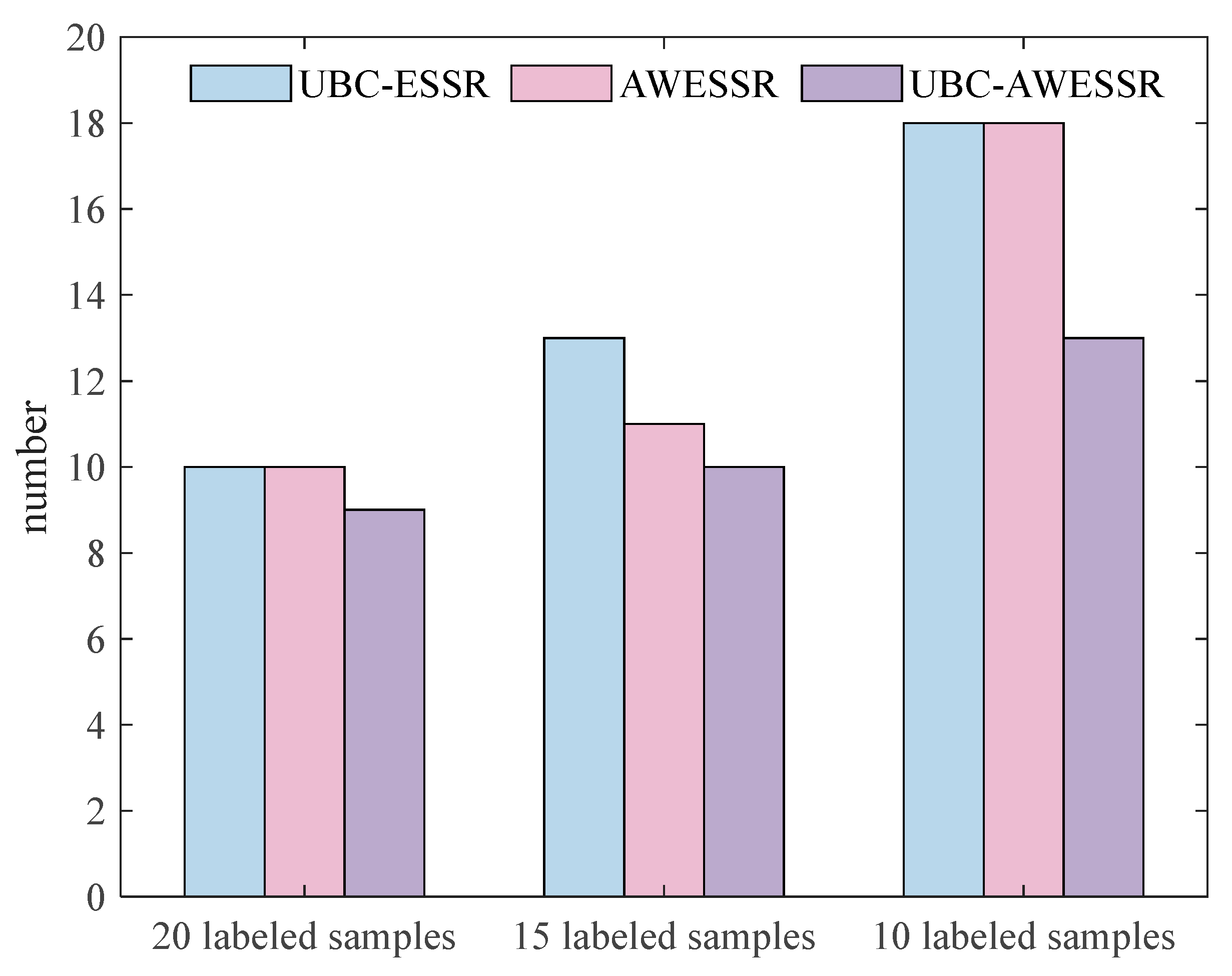
The influence of the pseudo-label screening method based on UBC on model performance

Table 4. Comparison results of AWESSR and UBC-AWESSR in cabin model experiment.

	MAE/dB			RMSE/dB
Number of Labeled Data	10	15	20	10	15	20
AWESSR	4.83	3.29	2.38	5.63	4.04	2.91
UBC-AWESSR	2.01	1.68	1.47	2.64	2.59	1.93
Error decreases	58.4%	48.9%	38.2%	53.1%	35.9%	33.7%

shows the comparison results of the UBC-AWESSR method in this paper with the AWESSR after removing UBC. After adding UBC, the prediction accuracy of the model effectively improves. When the number of label samples is only 10, the MAE and RMSE decrease the most, which are 58.4% and 53.1%, respectively. At this point, the performance improvement of the UBC is the most obvious.

The comparative result of prediction errors from the ablation tests when predicting URN of 1/3 oct frequency bands is shown in Figure 8, which reveals that UBC-AWESSR has the optimal prediction performance, followed by AWESSR and then UBC-ESSR. The number of bands with the error exceeding 3 dB is shown in Figure 9. These results confirm that the AWE method integrating anti-perturbation regularization exerts the most significant influence on prediction accuracy, with its removal causing severe performance degradation. Meanwhile, it shows that mitigating data disturbance constitutes a pivotal factor in determining model precision.

4.4.2. Experiment on the Research Vessel

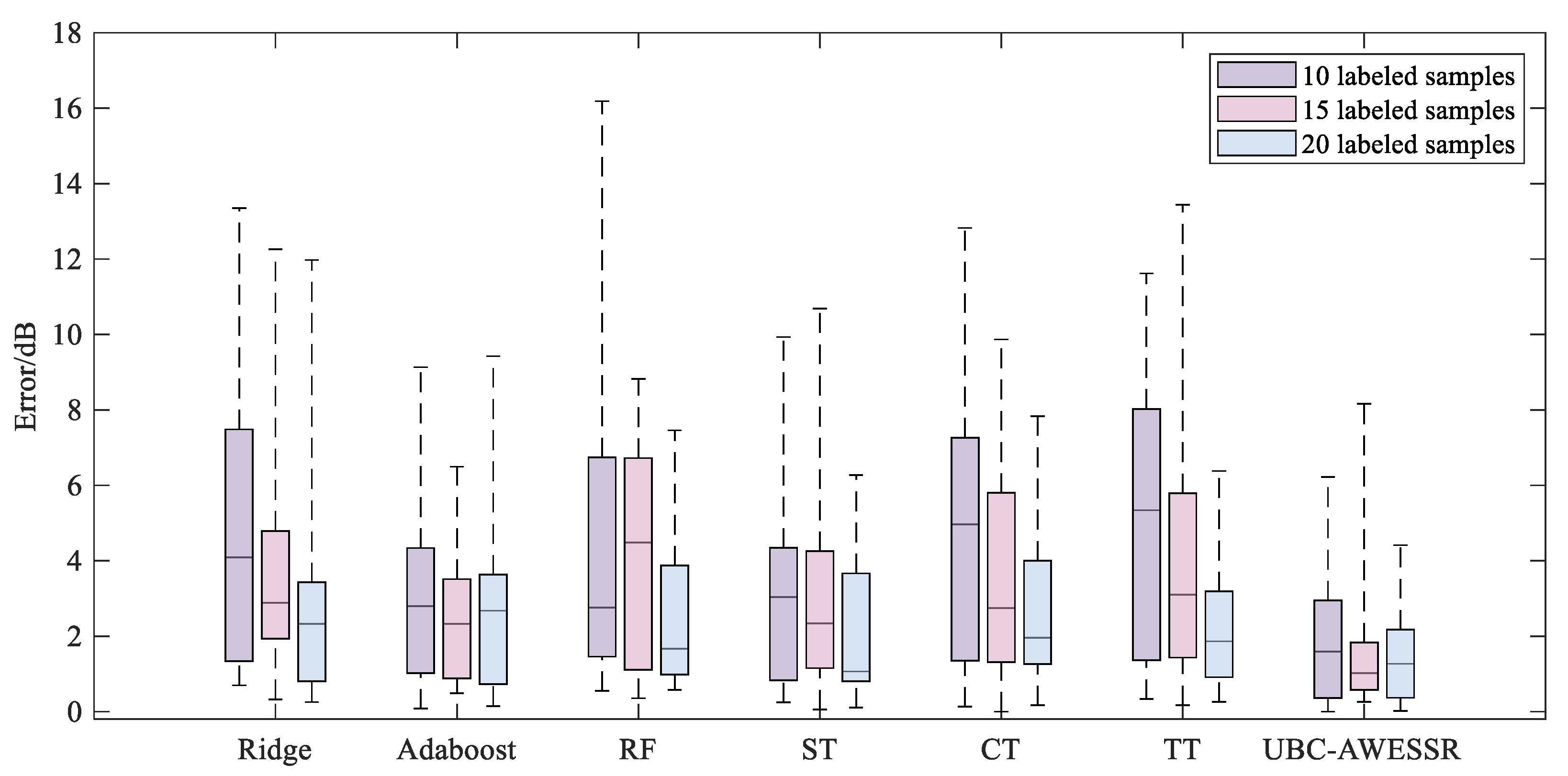
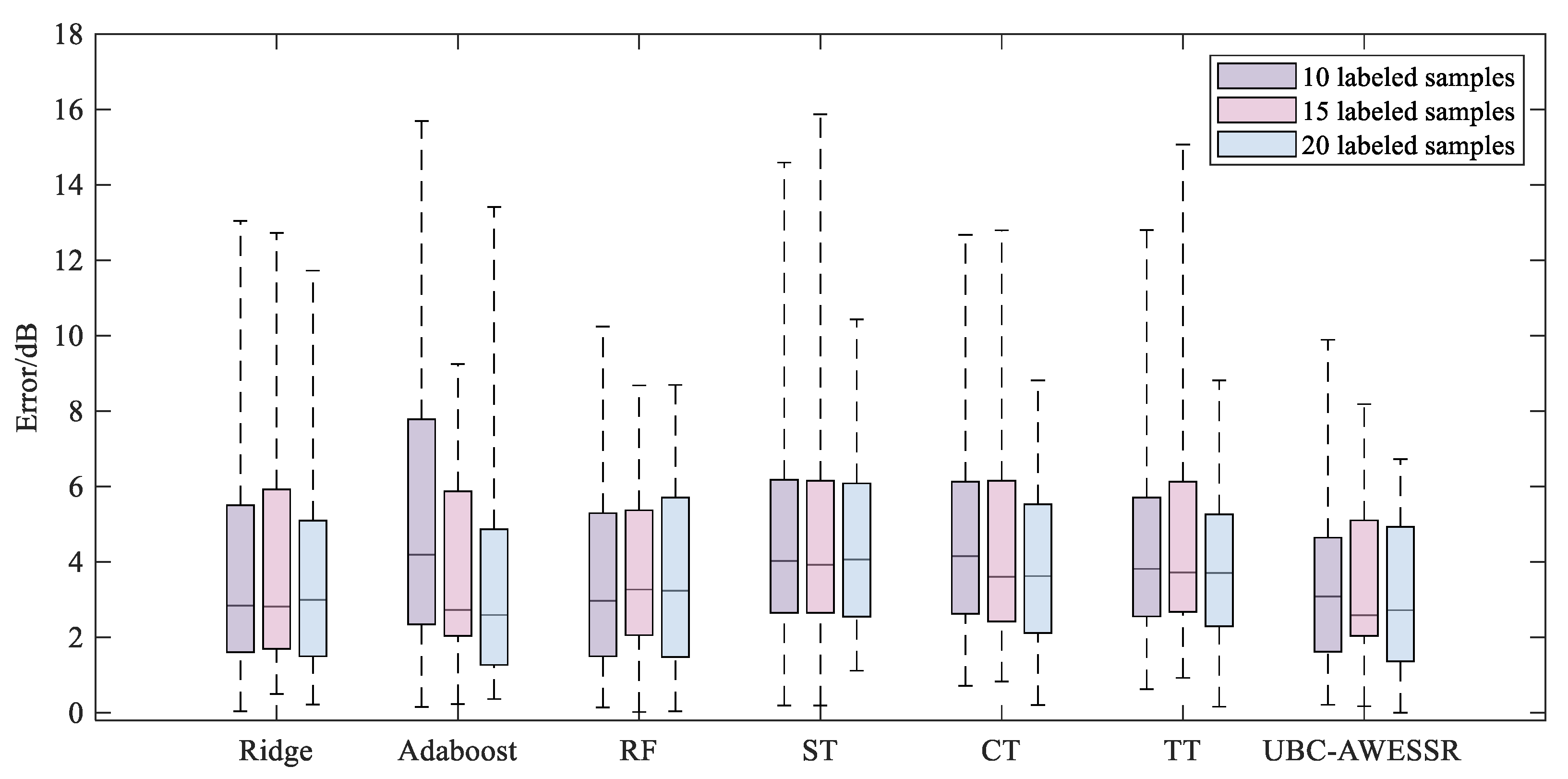
• Comparison of prediction results from different models

The lake test environment exhibits relatively clean background noise, whereas sea trials face more complex experimental conditions due to human activities, other vessel traffic, and marine life, posing greater challenges to data quality. As shown in Figure 10, the power spectrum density (PSD) of hull vibration signals collected during vessel trials reveals single-frequency interference contaminating the vibration inputs to the prediction model. These interferences partially distort the spectral characteristics of normal signals. Although subsequent filtering was applied, the influence of the interfering signal cannot be eliminated completely.

As presented in

Table 5. Predicted results of the research vessel.

		MAE/dB			RMSE/dB
Number of Labeled Data		10	15	20	10	15	20
SR	Ridge	3.90	4.08	3.68	5.02	5.08	4.61
	MLP	4.68	4.54	3.40	6.75	5.98	4.17
	Adaboost	5.23	3.95	3.49	6.55	4.79	4.63
	RF	3.81	3.88	3.60	4.92	4.60	4.41
SSR	ST	4.69	4.77	4.53	5.64	6.09	5.22
	CT	4.73	4.54	3.84	5.63	5.50	4.42
	TT	4.57	4.69	3.92	5.56	5.70	4.49
Proposed by us	UBC-AWESSR	3.69	3.63	3.04	4.69	4.36	3.66

, the proposed method maintains superior performance in predicting the vessel URN even under poor data quality conditions. Maximum reductions of 29.50% in MAE and 28.40% in RMSE were observed compared to conventional SR and SSR methods across three labeled sample quantities. These results robustly validate the method’s generalizability and robustness in complex maritime acoustic environments.

Figure 11 is a boxplot of the prediction error of radiated noise from surface ships. By comparing different models, both the maximum prediction error and the average prediction error under the UBC-AWESSR method are the smallest, which proves that the method proposed in this paper has a better prediction effect on the URN of vessels during navigation.

b.

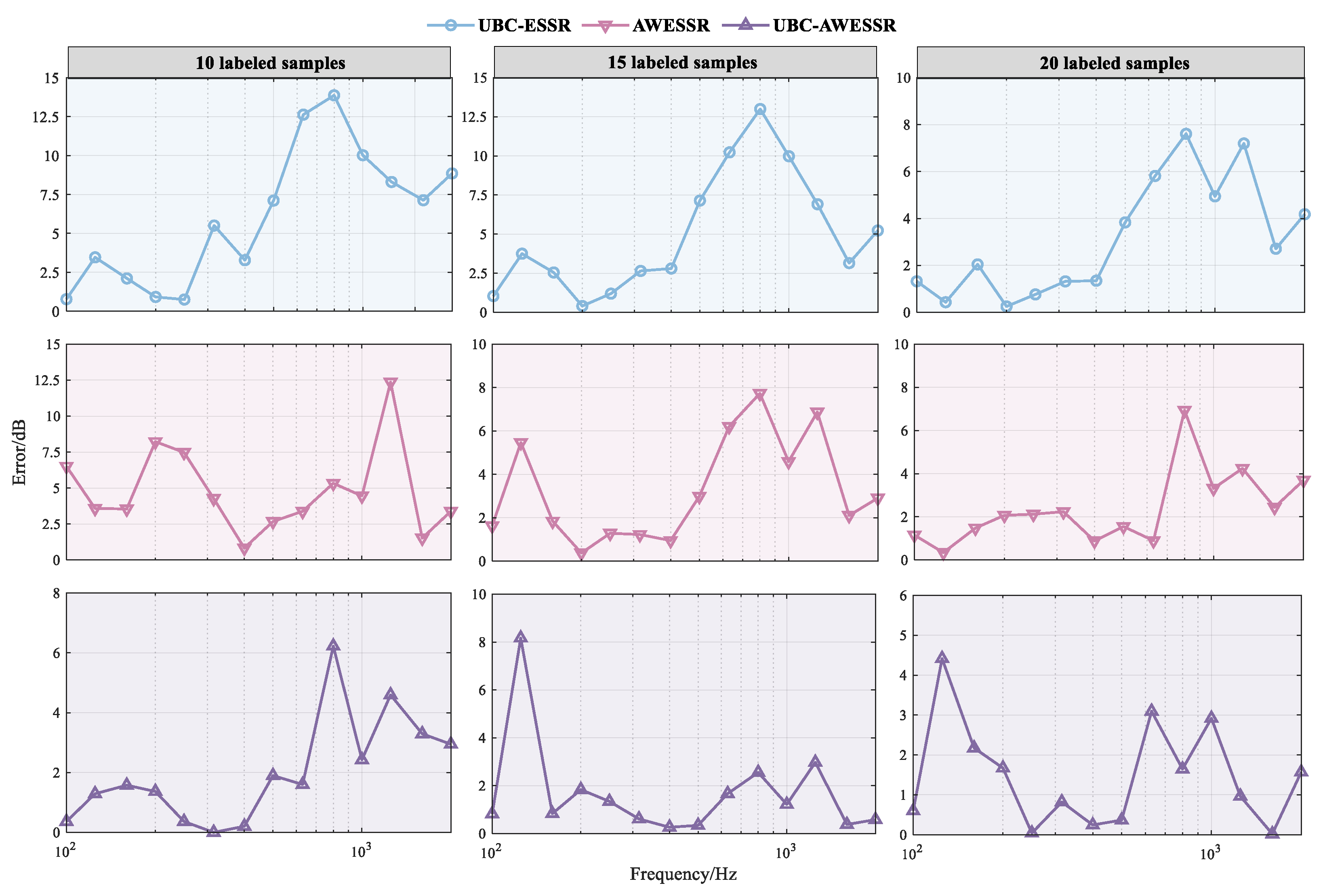
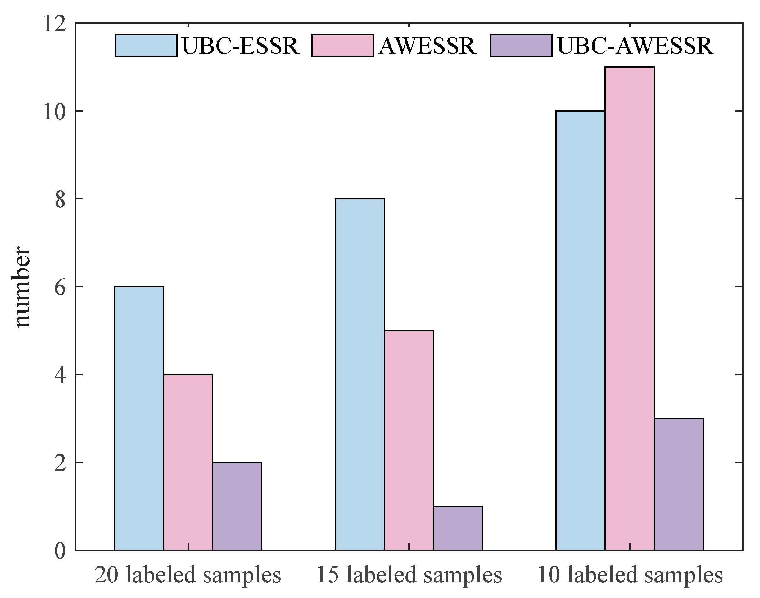
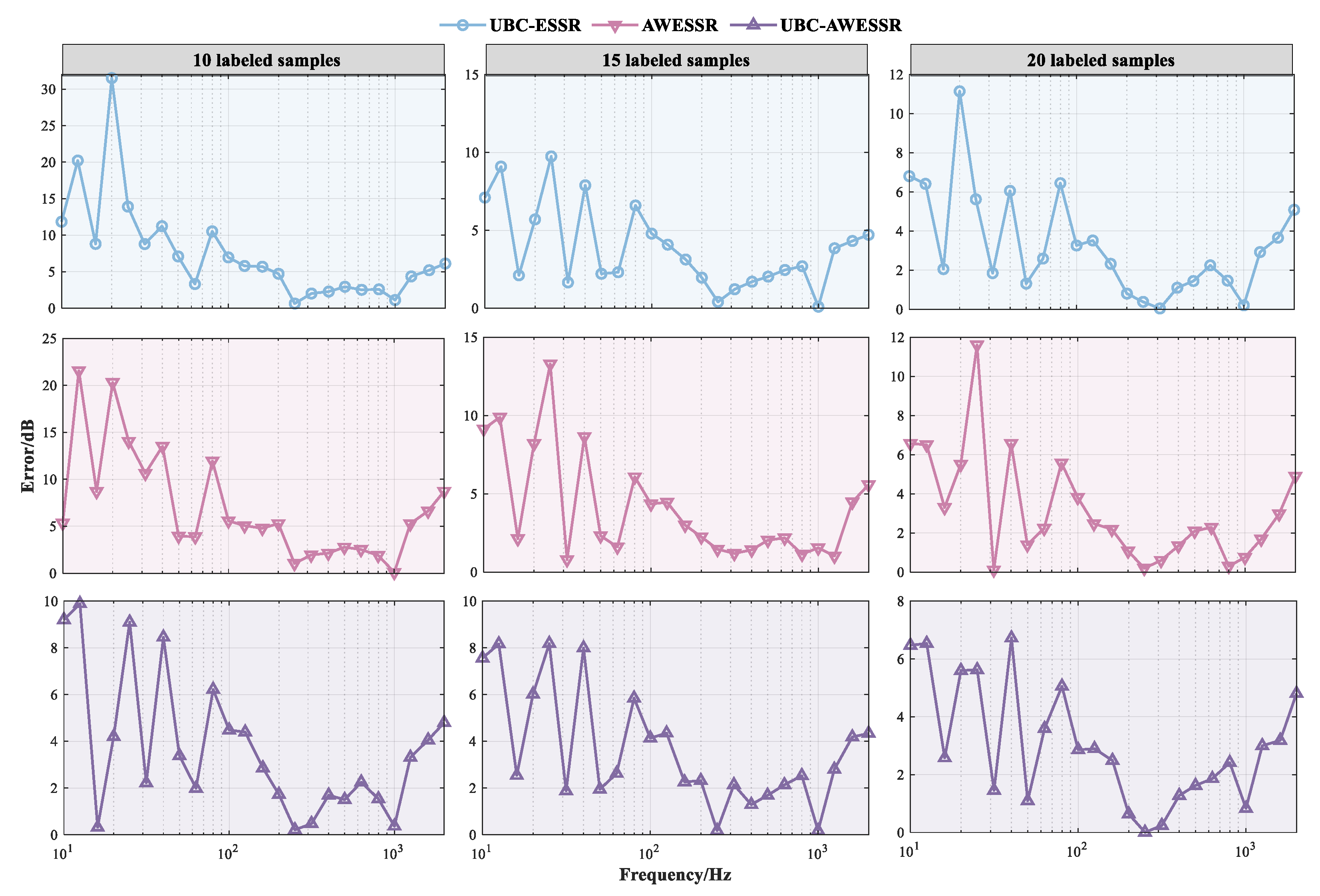
Ablation test results

To prove the validity of the two innovation points proposed in this paper, ablation tests were carried out, respectively, for comparative analysis.

(1)

The influence of AW based on the genetic algorithm on model performance

As demonstrated in

Table 6. Comparison results of UBC-ESSR and UBC-AWESSR in vessel experiment.

	MAE/dB			RMSE/dB
Number of Labeled Data	10	15	20	10	15	20
UBC-ESSR	7.50	3.83	3.28	10.08	4.63	4.21
UBC-AWESSR	3.69	3.63	3.04	4.69	4.36	3.66
Error decreases	50.8%	5.22%	7.32%	53.5%	5.83%	13.1%

, the UBC-ESSR model (without AW) exhibits severe performance degradation when labeled samples are reduced to 10, highlighting the substantial impact of AW on prediction robustness. Compared to UBC-ESSR, the integration of adaptive weighting in UBC-AWESSR achieves maximum reductions of 50.8% in MAE and 53.5% in RMSE under the 10 labeled samples. This contrast validates the critical role of AW in mitigating performance deterioration caused by extreme data scarcity.

(2)

The influence of the pseudo-label screening method based on UBC on model performance

As evidenced in

Table 7. Comparison results of AWESSR and UBC-AWESSR in vessel experiment.

	MAE/dB			RMSE/dB
Number of Labeled Data	10	15	20	10	15	20
AWESSR	6.98	4.09	3.17	8.97	5.30	4.17
UBC-AWESSR	3.69	3.63	3.04	4.69	4.36	3.66
Error decreases	47.1%	11.3%	4.10%	47.8%	17.7%	12.2%

, the UBC mechanism significantly enhances prediction precision when comparing UBC-AWESSR and its variant AWESSR (without UBC). Under the condition of only 10 labeled samples, UBC-AWESSR achieves maximum reductions of 47.10% in MAE and 47.80% in RMSE, demonstrating the most pronounced performance improvement. These results validate the critical role of UBC in compensating for uncertainty-induced deviations, particularly in ultra-low labeled data regimes.

As shown in Figure 12 and Figure 13, the comparative prediction results of the three ablation groups reveal that UBC-AWESSR has the optimal performance, followed by AWESSR and UBC-ESSR, respectively. Consistent with results from the cabin model, the proposed method demonstrates its most pronounced advantage under extremely limited sample conditions.

As shown in Figure 12, prediction errors exceeding 3 dB across the UBC-ESSR, AWESSR, and UBC-AWESSR models predominantly cluster within the 10–100 Hz low-frequency band, likely attributed to data distribution inconsistency. Given the unknown training-testing sample distribution, we employ the nonparametric Kolmogorov–Smirnov (KS) test to quantify distributional consistency. The KS statistic derives from the maximum divergence $D_{n,m}$ between the empirical cumulative distribution functions (CDFs) of two samples. A higher p-value indicates a stronger likelihood of shared distributions, while p-values below the significance threshold we reject the same distribution. The p-value calculation follows Equation (15).

$$p=2e^{-2{\left(D_{n,m}\right)}^2{\displaystyle \frac{n\ast m}{n+m}}}$$

(15)

Here, n and m denote the training and testing sample sizes, respectively, and $\alpha$ represents the significance level; we set $\alpha =5\%$ in this study. As shown in Figure 14, the KS test p-values for different 1/3 oct bands reveal distinct distributional characteristics. In high-frequency bands, p-values predominantly exceed 0.6, supporting the hypothesis of shared distributions between training and testing samples. Conversely, low-frequency bands exhibit markedly lower p-values (around 0.2), indicating weaker distributional consistency. This divergence statistically explains the high prediction errors in the low-frequency range, where model performance is compromised by distributional mismatches.

Figure 15 presents the KS test results comparing training samples augmented with pseudo-labeled data and testing samples. In contrast to Figure 14, the high-frequency bands (>25 Hz) show negligible changes in p-values, while the low-frequency regime (<25 Hz) exhibits a modest p-value increase. Correspondingly, prediction errors decrease marginally in low frequencies but remain stable at higher frequencies. These observations demonstrate the limited efficacy of semi-supervised strategies under current data constraints, where experimental datasets fail to encompass full distributional diversity. This limitation underscores the necessity of integrating physics-informed constraints and prior knowledge to guide model training, which is a critical direction for future research outlined in this work.

5. Conclusions

This paper proposes a new semi-supervised ensemble learning model, UBC-AWESSR, for evaluating ship URN. This model consists of three parts, which are an adaptive weighted ensemble based on genetic algorithm, dynamic pseudo-label screening, and uncertainty bias correction. It can effectively improve the prediction performance of the model under limited label data. The main conclusions are as follows:

(1)

We designed cabin model experiment and vessel experiment to verify the effectiveness of UBC-AWESSR model, and the results showed that UBC-AWESSR can reduce MAE and RMSE by up to 65.5% and 69.4% compared with the traditional SR and SSR models.

(2)

The predictive performances of different models under different numbers of labeled samples were compared. The results show that the fewer the number of labeled samples, the more obvious the advantages of UBC-AWESSR model become.

(3)

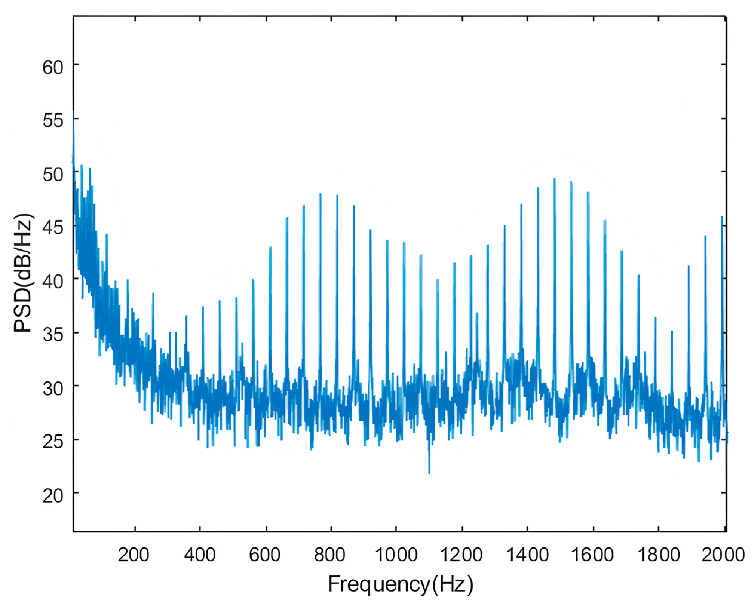
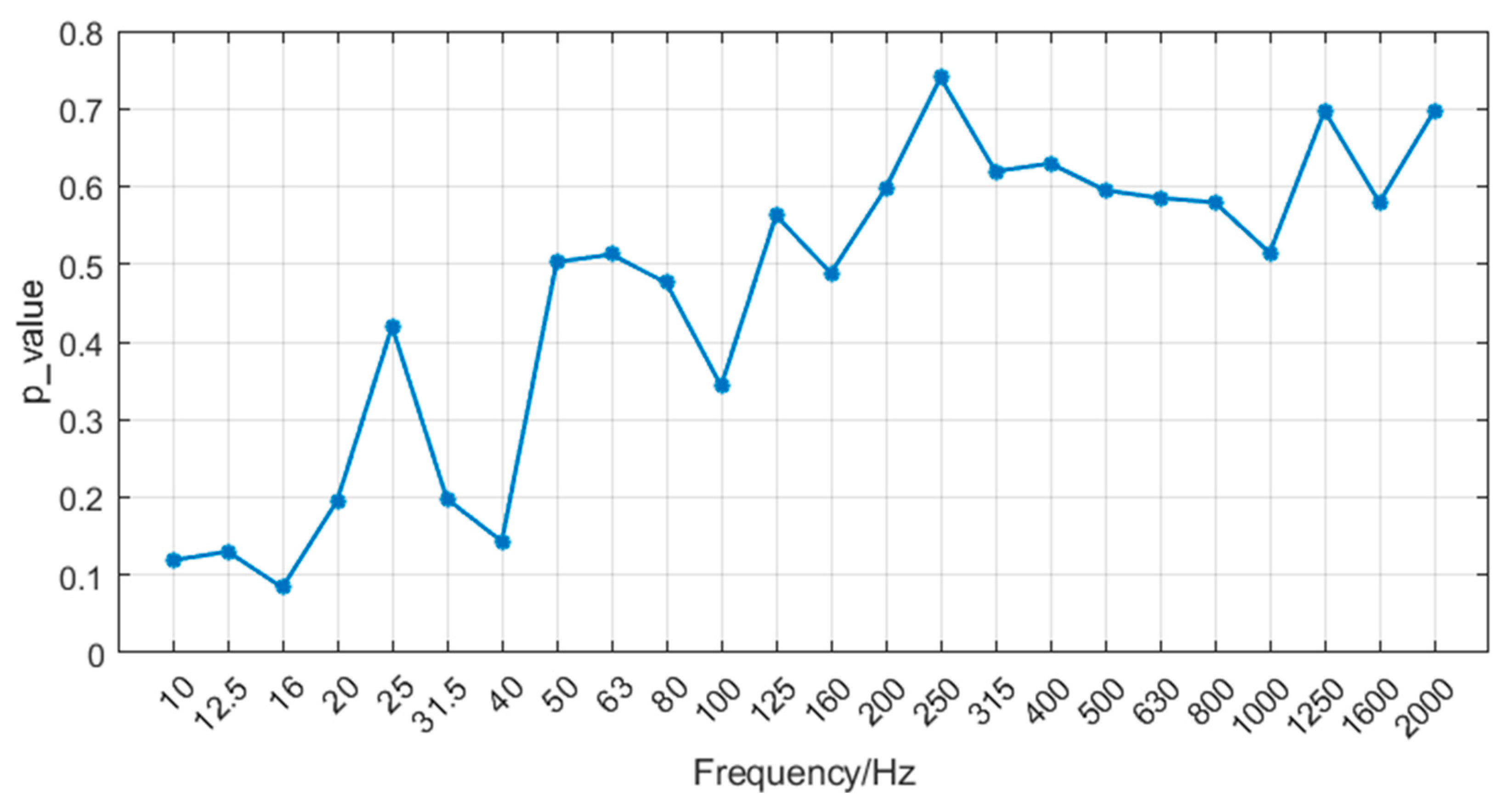
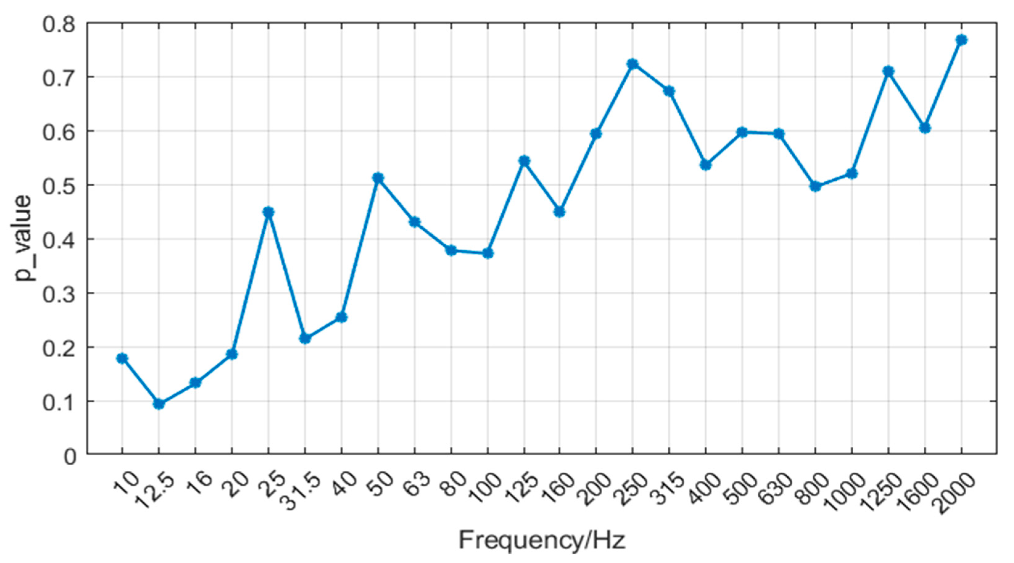
The experimental data collected during the sea trial contained single-frequency interference signals. However, even when the data quality was poor, UBC-AWESSR model still exhibited a relatively good predictive effect.

(4)

The results of the ablation tests show that the AWE integrating anti-perturbation regularization has the most significant impact on the model prediction, and the model performance degrades severely after removal, which provides supporting evidence for conclusion (3) from a different perspective.

(5)

To obtain more useful information to assist model training and increase the interpretability of the model, the data-driven integrating physical knowledge is the future research direction and the next focus of this paper.

References

- Meng, X.Y.; Xiao, G.L.; Chen, H. Review of Current Status and Development of Submarine Acoustic Stealth Technology Abroad. J. Ship Sci. Technol. 2011, 33, 135–139. [Google Scholar]
- Jiang, L.G. 21st-Century Naval Vessels; National Defense Industry Press: Beijing, China, 1988. [Google Scholar]
- Sun, X.R.; Zhu, X. Survey and Tendency of Study on the Underwater Noise of Ship Structure. J. Vib. Shock 2005, 1, 108–115. [Google Scholar]
- Cui, W.C.; Liu, S.G.; Gu, J.H.; Li, Z.Y. Some New Trends on Submarine Design and Performance Studies Abroad. J. Ship Mech. 2000, 2, 65–80. [Google Scholar]
- Guo, W.J.; Li, T.Y.; Zhu, X.; Miao, Y.Y. Acoustic analysis of a finite cylindrical shell in an acoustic half-space based on Fourier transform technique. J. Vib. Eng. Technol. 2019, 7, 611–627. [Google Scholar] [CrossRef]
- Guo, W.J.; Li, T.Y.; Zhu, X.; Miao, Y.Y. Vibro-acoustic analysis of the thin laminated rectangular plate-cavity coupling system. Compos. Struct. 2018, 189, 570–585. [Google Scholar]
- Zhang, L.; Duan, J.-X.; Da, L.-L.; Xu, G.-J.; Sun, X.-H. Vibroacoustic radiation and propagation properties of slender cylindrical shell in uniform shallow sea. Ocean Eng. 2020, 195, 106659. [Google Scholar] [CrossRef]
- Kim, S.M.; Brennan, M.J. A compact matrix formulation using the impedance and mobility approach for the analysis of structural-acoustic systems. J. Sound Vib. 1999, 223, 97–113. [Google Scholar] [CrossRef]
- Zhang, B.; Xiang, Y.; He, P.; Zhang, G.-J. Study on prediction methods and characteristics of ship underwater radiated noise within full frequency. Ocean Eng. 2019, 174, 61–70. [Google Scholar] [CrossRef]
- Li, D.-Q.; Hallander, J.; Johansson, T. Predicting underwater radiated noise of a full scale ship with model testing and numerical methods. Ocean Eng. 2018, 161, 121–135. [Google Scholar] [CrossRef]
- Viitanen, V.; Hynninen, A.; Sipilä, T. Computational fluid dynamics and hydroacoustics analyses of underwater radiated noise of an ice breaker ship. Ocean Eng. 2023, 279, 114264. [Google Scholar] [CrossRef]
- Kim, S.; Kinnas, S.A. Numerical prediction of propeller-induced noise in open water and ship behind conditions. Ocean Eng. 2022, 261, 112122. [Google Scholar] [CrossRef]
- Özden, M.C.; Gürkan, A.Y.; Ozden, M.C.; Canyurt, T.G.; Korkut, E. Underwater radiated noise prediction for a submarine propeller in different flow conditions. Ocean Eng. 2016, 126, 488–500. [Google Scholar] [CrossRef]
- Wang, B. Research on Prediction of Noise Radiated by Large Underwater Structure Via Surface Vibration Monitoring. Ph.D. Thesis, Shanghai Jiao Tong University, Shanghai, China, 2008. [Google Scholar]
- Cintosun, E. Derivations of transfer functions for estimating ship underwater radiated noise from onboard vibrations. Ocean Eng. 2024, 311, 118792. [Google Scholar] [CrossRef]
- Ye, L.; Shen, J.; Tong, Z.; Liu, Y. Research on acoustic reconstruction methods of the hull vibration based on the limited vibration monitor data. Ocean Eng. 2022, 266, 112886. [Google Scholar] [CrossRef]
- Park, U.; Kang, Y.J. Operational transfer path analysis based on neural network. J. Sound Vib. 2024, 579, 118364. [Google Scholar] [CrossRef]
- Zhang, X.Z.; Yang, H.C. To Predict the Radiation Noise of Ship Based on RBF Neural Network. Value Eng. 2011, 30, 62–63. [Google Scholar]
- Tang, Z.Y.; Li, G.H.; He, L. Acoustic stealth situation assessment of underwater vehicle based on fuzzy support vector machine. In Proceedings of the 2009 International Conference on Mechatronics and Automation, Changchun, China, 9–12 August 2009; pp. 2095–2100. [Google Scholar]
- Li, J.Y.; Pan, Y.; Wang, Q. Research on the Application of Deep Neural Network in Ship Radiated Noise Simulation. Acoust. Electron. Eng. 2022, 01, 10–15. [Google Scholar]
- Miglianti, L.; Cipollini, F.; Oneto, L.; Tani, G.; Gaggero, S.; Coraddu, A.; Viviani, M. Predicting the cavitating marine propeller noise at design stage: A deep learning based approach. Ocean Eng. 2020, 209, 107481. [Google Scholar] [CrossRef]
- Fan, B. Prediction of Cabin Noise for Offshore Platforms Based on Intelligent Algorithms. Master’s Thesis, Harbin Engineering University, Harbin, China, 2018. [Google Scholar]
- He, T.J. Research on Measurements of the Radiated Noise from Shipping in Shallow Water. Ph.D. Thesis, Harbin Engineering University, Harbin, China, 2022. [Google Scholar]
- Shahshahani, B.; Landgrebe, D. The effect of unlabeled samples in reducing the small sample size problem and mitigating the hughes phenomenon. IEEE Trans. Geosci. Remote Sens. 1994, 32, 1087–1095. [Google Scholar] [CrossRef]
- Liu, J.W.; Liu, Y.; Luo, X.L. Semi-supervised Learning Methods. Chin. J. Comput. 2015, 38, 1592–1617. [Google Scholar]
- Zhou, Z.H.; Li, M. Semisupervised regression with cotraining-style algorithms. IEEE Trans. Knowl. Data Eng. 2007, 19, 1479–1493. [Google Scholar] [CrossRef]
- Gan, H.T. Research on Semi-Supervised Clustering and Classification Algorithm. Ph.D. Thesis, Huazhong University of Science and Technology, Wuhan, China, 2014. [Google Scholar]
- Qin, Y.; Ding, S.; Wang, L.; Wang, Y. Research progress on semi-supervised clustering. Cogn. Comput. 2019, 11, 599–612. [Google Scholar] [CrossRef]
- Li, J.; Zhu, X.; Wang, H.; Zhang, Y.; Wang, J. Stacked co-training for semi-supervised multi-label learning. Inf. Sci. 2024, 677, 120906. [Google Scholar] [CrossRef]
- Kostopoulos, G.; Karlos, S.; Kotsiantis, S.; Ragos, O. Semi-supervised regression: A recent review. J. Intell. Fuzzy Syst. 2018, 35, 1483–1500. [Google Scholar] [CrossRef]
- Scudder, H.J. Probability of error of some adaptive pattern-recognition machines. IEEE Trans. Inf. Theory 1965, 11, 363–371. [Google Scholar] [CrossRef]
- Blum, A.; Mitchell, T. Combining labeled and unlabeled data with co-training. In Proceedings of the Eleventh Annual Conference on Cozmputational Learning Theory, Madison, WI, USA, 24–26 July 1998; pp. 92–100. [Google Scholar]
- Zhou, Z.H.; Li, M. Semi-supervised regression with co-training. In Proceedings of the 19th International Joint Conference on Artificial Intelligence (IJCAI), Edinburgh, UK, 30 July–5 August 2005; pp. 908–913. [Google Scholar]
- Zhou, Z.H. Tri-training: Exploiting unlabeled data using three classifiers. IEEE Trans. Knowl. Data Eng. 2005, 17, 1529–1541. [Google Scholar] [CrossRef]
- Li, M.; Zhou, Z.H. Improve computer-aided diagnosis with machine learning techniques using undiagnosed samples. IEEE Trans. Syst. Man Cybern. Part A Syst. Hum. 2007, 37, 1088–1098. [Google Scholar] [CrossRef]
- Zhou, Z.H. When semi-supervised learning meets ensemble learning. Front. Electr. Electron. Eng. China 2011, 6, 6–16. [Google Scholar] [CrossRef]
- Miyato, T.; Maeda, S.-I.; Koyama, M.; Ishii, S. Virtual adversarial training: A regularization method for supervised and semi-supervised learning. IEEE Trans. Pattern Anal. Mach. Intell. 2018, 41, 1979–1993. [Google Scholar] [CrossRef]
- Meel, P.; Vishwakarma, D.K. A temporal ensembling based semi-supervised ConvNet for the detection of fake news articles. Expert Syst. Appl. 2021, 177, 115002. [Google Scholar] [CrossRef]
- Zhou, Z.H.; Li, M. Semi-supervised learning by disagreement. Knowl. Inf. Syst. 2010, 24, 415–439. [Google Scholar] [CrossRef]
- Huang, X.; Xu, R.; Li, R. An Online Prediction Method for Ship Underwater Radiated Noise Based on Differential Evolution Feature Optimization and Ensemble Method. Ocean Eng. 2025, 333, 121517. [Google Scholar] [CrossRef]
- Montgomery, D.C.; Peck, E.A.; Vining, G.G. Introduction to Linear Regression Analysis; China Machine Press: Beijing, China, 2016; p. 35. [Google Scholar]