Wave Run-Up Distance Prediction Combined Data-Driven Method and Physical Experiments

Abstract

Predicting wave run-up on seawalls is essential for assessing coastal flood risk and guiding resilient design. In this study, we combine physical model experiments with a hybrid data driven method to forecast wave run-up distance. Laboratory tests generated a nonlinear data set spanning a wide range of wave amplitudes, wavelengths, Froude numbers. To capture the underlying physical regimes, the records were first classified using a Gaussian Mixture Model (GMM), which automatically grouped waves of similar hydrodynamic character. Within each cluster a Gradient Boosting Regressor (GBR) was then trained, allowing the model to learn tailored input–output relationships instead of forcing a single global fit. Results demonstrate that the GMM-GBR combined model achieves a coefficient of determination $R^2$ greater than 0.91, outperforming a conventional, non-clustered GBR model. This approach offers a reliable tool for predicting seawall performance under varying wave conditions, contributing to better coastal management and resilience strategies.

1. Introduction

Coastal areas are increasingly vulnerable to the impacts of extreme waves and tsunamis, necessitating effective protective measures to safeguard these areas. Seawalls are a primary defence mechanism designed to shield coastal zones from the intrusion of seawater [1,2,3]. However, during extreme wave events, seawalls may be overtopped, leading to significant coastal flooding and shoreline alterations [4]. Understanding and predicting the characteristics of waves interacting with seawalls are thus paramount for effective coastal risk management. Among the various parameters influencing coastal inundation, the wave run-up distance on seawalls emerges as a critical factor contributing to coastline flooding.

Extensive researches have been conducted to elucidate the dynamics of wave run-up on seawalls, employing a range of methodologies such as physical model experiments, analytical models, numerical simulations and field monitoring [5,6,7,8,9]. Physical model experiments, in particular, have proven to be one of the most effective approaches for capturing the complex interactions between waves and coastal structures. Over the years, numerous empirical formulas have been developed based on experimental data to predict wave run-up characteristics [10,11,12,13]. Despite these advancements, significant discrepancies often persist between predicted and observed run-up values, fueling ongoing debates regarding the most reliable parameterizations for accurately describing wave run-up phenomena. Analytical models offer simplified representations of wave-seawall interactions by applying fundamental fluid dynamics principles, yet they often struggle to account for the full complexity of real-world scenarios [14,15,16,17,18]. Numerical simulations provide detailed insights by solving the governing equations of fluid motion but require substantial computational resources and expertise [19,20,21]. Field monitoring collects in-situ data from coastal environments, which often serves as a method for developing prediction models and understanding wave-seawall interactions in real-world [22].

In addition to these primary methods, various alternative approaches have been explored in the literature to enhance the prediction of wave run-up. For example, hybrid models that combine empirical data with numerical techniques have also been widely applied, so as to leverage the advantage of each method [23,24,25]. Statistical methods also have been applied to assess the likelihood of extreme run-up events [26,27]. Achieving high accuracy and reliability in wave run-up distance predictions remains a challenge, highlighting the need for innovative methodologies that can effectively integrate various sources of information and handle the inherent variability of coastal wave dynamics.

In recent years, with the development of computational techniques, researchers start to enhance the prediction of wave run-up distance on seawall through applying machine learning methods, which offer the potential to capture intricate patterns and nonlinear relations inherent in wave dynamics [28,29,30,31,32]. Previous attempts which integrate machine learning techniques into wave run-up prediction have demonstrated promising results, while challenges still exist in achieving robust performance across varying wave conditions [33,34,35,36]. A critical factor influencing the wave run-up prediction accuracy is the non-linearity of waves [37]. Different wave characteristics, such as height, period, and steepness, can significantly affect the interaction dynamic of wave and seawalls, thereby impacting the wave run-up distance [38,39]. Consequently, developing prediction models that account for distinct wave features is essential for achieving high-performance prediction methods.

To consider the influence of wave feature in modeling, we proposed a wave run-up prediction model combining Gaussian mixture model (GMM) and gradient boosting regression (GBR) [40,41,42]. The focus of the study is the incorporation of GMM clustering to partition the experimental wave data into hydrodynamically distinct regimes before regression. By assigning each observation to a Gaussian component—each representing a specific wave class, the subsequent GBR models can be trained on regime-specific subsets, yielding more accurate and interpretable predictions of run-up behavior. While recent hybrid physics–machine learning studies have demonstrated the value of combining laboratory experiments and data-driven methods, none exploit GMM-based regime separation to enhance both accuracy and interpretability in wave run-up modeling as we do here [43,44,45]. In the present study, we first conduct experiments to mimic wave run-up distance on seawall under different wave conditions. As the wave characteristics exhibit inherent complexity and variability, we employ the GMM to cluster the dataset into several groups based on their features. Each group represents specific wave characteristics [46]. Then, we train the GBR to predict the run-up distance on seawall for each cluster, taking the advantage of machine learning in handling nonlinear relation modeling. By developing the GMM-GBR hybrid model, we aim to advance the predictive capabilities for wave run-up distance, and thereby give support to coastal risk management.

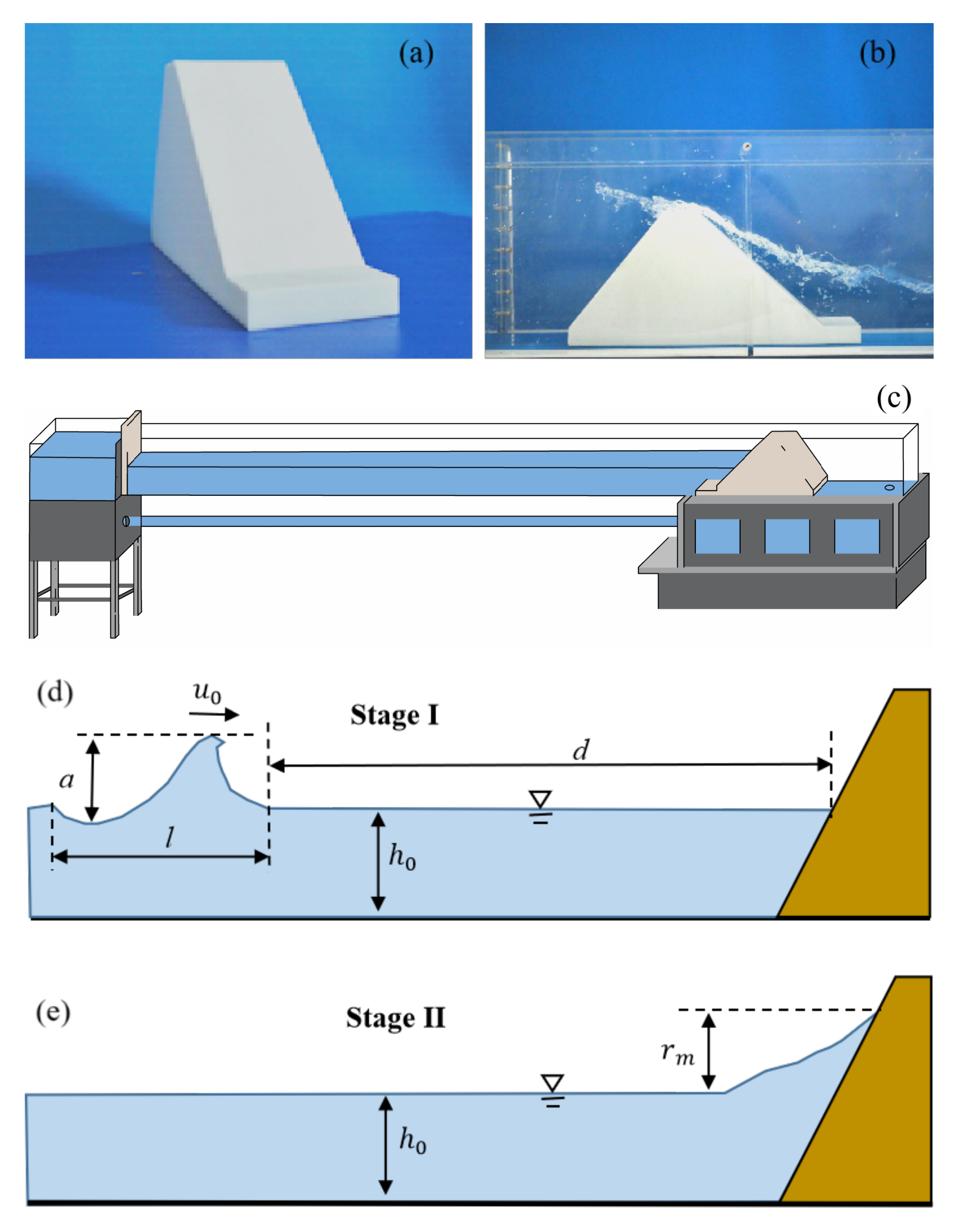
2. Physical Model Experiments

As shown in Figure 1, tests were carried out in a narrow flume that is 3 m long, 0.15 m wide and 0.40 m deep. A reservoir on the left releases water once its gate is lifted, generating a single wave that travels down-flume and hits a model seawall on the right. The release volume and gate-open time determine the wave’s amplitude, length and peak velocity. The seawall is 30 cm wide at the base, 25 cm high and inclined at 45°, dimensions chosen to mimic a typical coastal revetment. Two high-speed cameras capture the flow: a 1280 × 2400-pixel camera records the full wave path, while a 600 × 800-pixel camera focuses on the run-up zone. Both operate at 200 frames per second. A 0.20 m × 0.20 m calibration grid converts image pixels to physical distances. A total of 156 experimental runs were conducted across the full range of test conditions. Measurements were recorded at two stages: Stage I (Figure 1d) captured the incident-wave characteristics—wave amplitude a, peak flow velocity $u_0$, wavelength l, and still-water depth $h_0$. Stage II (Figure 1e) focused on the maximum run-up distance on the seawall $r_m$. Systematically varying a, $u_0$, l and $h_0$ produces a broad data set for developing predictive models of run-up behaviour. Although our flume is only 3 m long which is adequate for Froude-scaled, short-period wind-wave studies, note that this setup cannot reproduce longer-period swell or fully irregular sea states. These are beyond the scope of the present proof-of-concept.

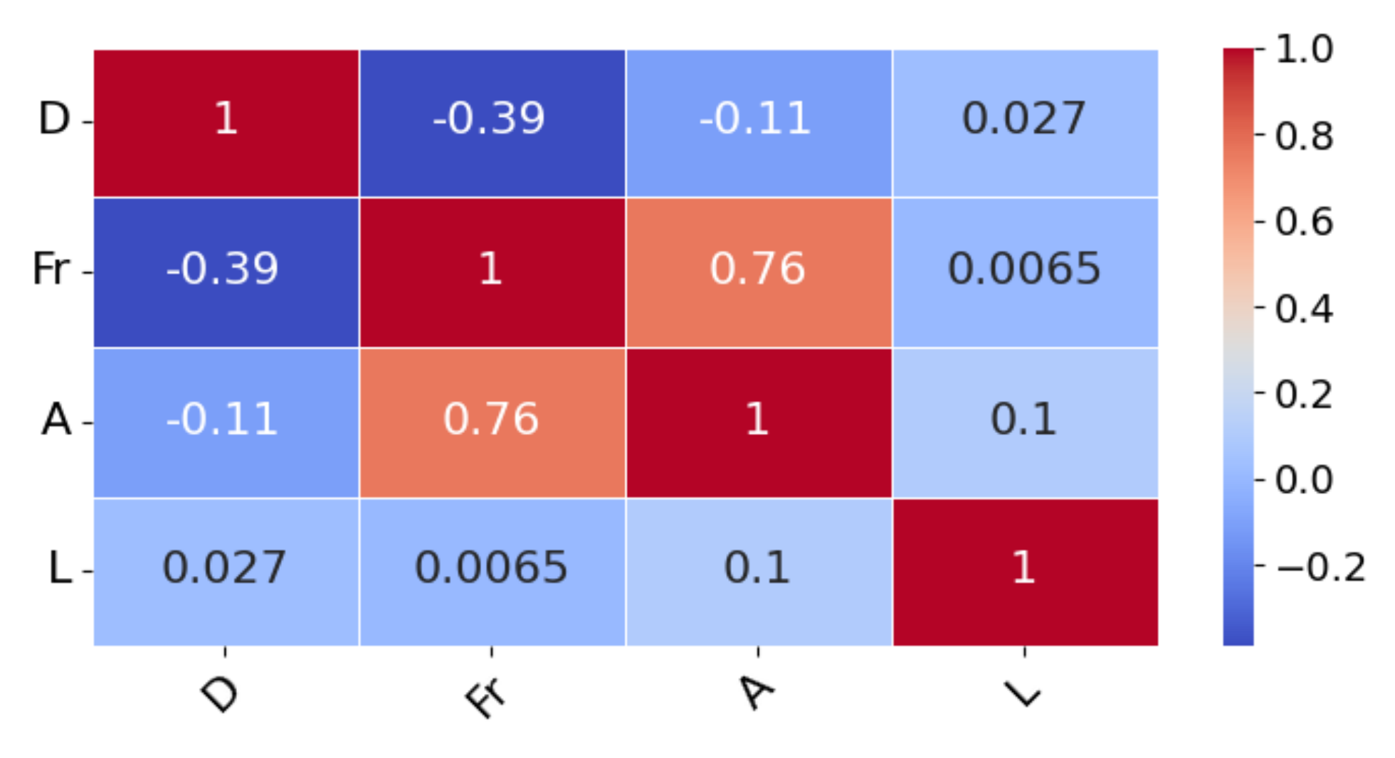
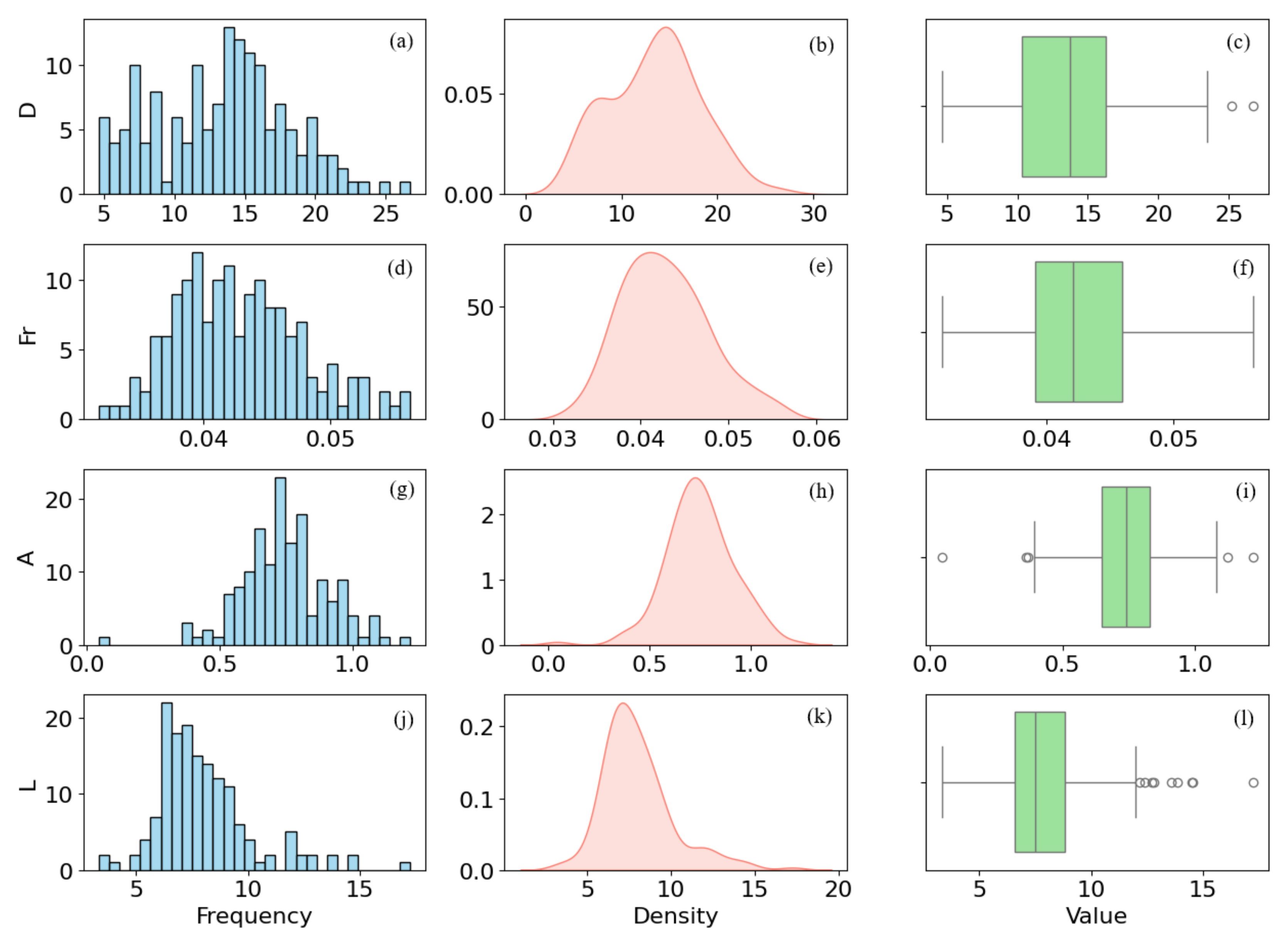
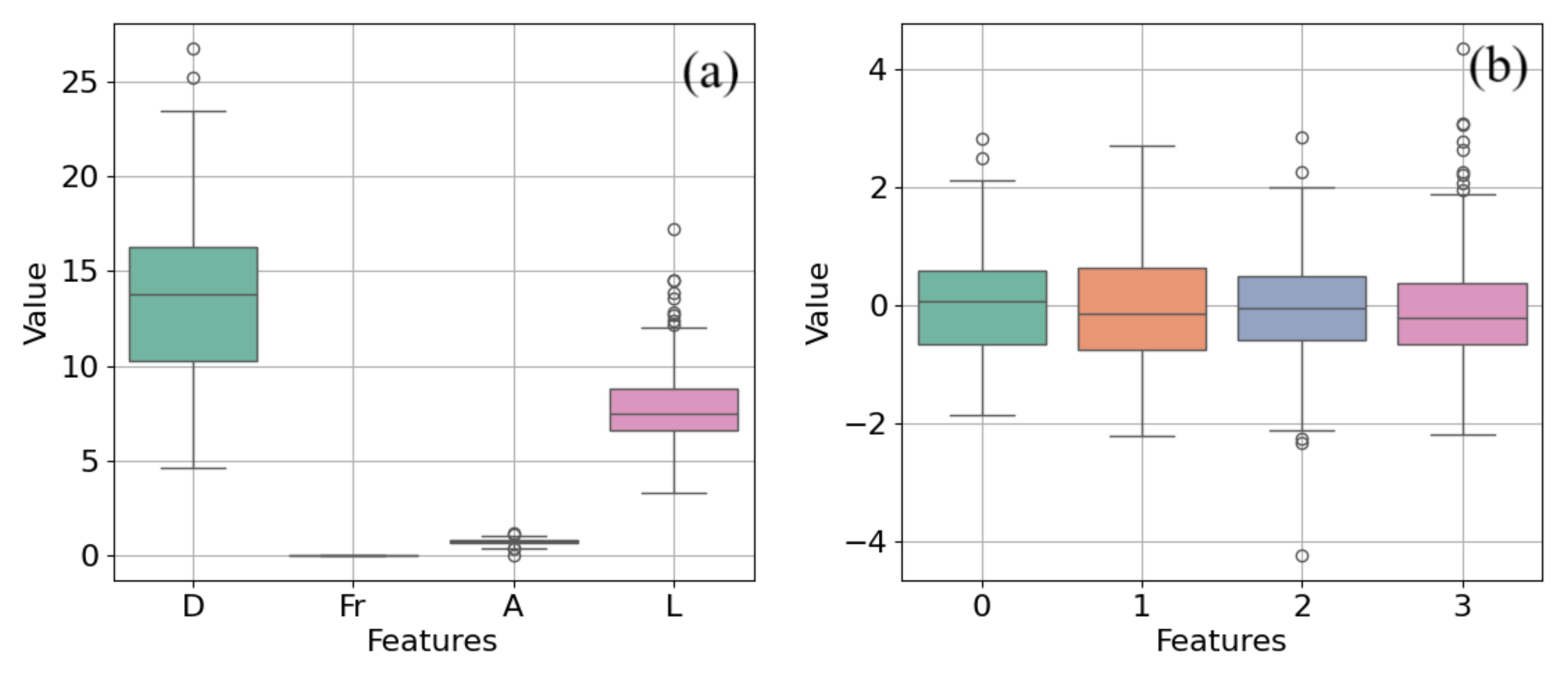
3. Dimensionless Analysis

As introduced in Section 2, $r_m$ is governed primarily by four variables: a, l, $u_0$, and d. This dependence can be summarized as:

$$r_m=\mathit{f}(a,d,l,u_0)$$

(1)

For clearer comparison of experimental results, each variable is recast in dimensionless form using the still-water depth $h_0$ as the reference scale. Here, we introduce:

$$A={\displaystyle \frac{a}{h_0}},L={\displaystyle \frac{l}{h_0}},\mathrm{Fr}={\displaystyle \frac{u_0}{\sqrt{g{h}_0}}},D={\displaystyle \frac{d}{h_0}},R={\displaystyle \frac{r_m}{h_0}}.$$

(2)

where A represents the relative wave amplitude, L the relative wave length, Fr the Froude number, D the normalized distance to the seawall, and R the normalized run-up distance. Expressed with these nondimensional groups, the input–output relationship becomes

$$R=\mathit{f}(A,L,\mathrm{Fr},D)$$

(3)

A correlation analysis was conducted to confirm the chosen of input variables Fr, D, A and L, as depicted in Figure 2. The results indicate a positive correlation between the Fr and A with a Pearson correlation coefficient of 0.76, suggesting that increases in Fr are associated with increases in A. The correlations among the other variables (Fr and D, Fr and L, D and A, D and L, A and L) are all below 0.4, indicating weak linear relationships and minimizing concerns about multicollinearity among these pairs. That is, the selected variables exhibit high levels of intercorrelation, supporting their inclusion in the model.

Figure 3 presents the distribution of four parameters (i.e., D, Fr, A, and L) using a combination of vertical histograms, kernel density estimation (KDE) plots. Each row corresponds to one parameter, with the first column displaying a histogram that illustrates the frequency distribution of the parameter values. The second column features a vertical KDE plot, providing a smooth estimation of the data density and highlighting the distribution’s shape and central tendencies. The third column contains a boxplot, summarizing the median, interquartile range (IQR), and identifying potential outliers for each parameter. D demonstrates a mean value of approximately 13.5, ranging from 4.6 to 26.7, with a median close to 13.0, indicating a moderately right-skewed distribution. The Fr exhibits a mean of 0.04, spanning from 0.03 to 0.05, and appears to follow a relatively symmetric distribution centered around the mean. A has a mean of 0.75, with values ranging between 0.3 and 1.22. scaled wave length L presents a mean of approximately 8.0, varying from 3.3 to 17.25, which reflects a broad distribution with potential outliers on the higher end.

4. Mathematical Principles of the GBR-GMM Combined Model

We initially classified the experimental data into several clusters using Gaussian mixture model (GMM), which enable us to identify the underlying patterns within the data based on their statistical properties and capture the inherent heterogeneity of the wave propagation. Considering the data distribute as a combination of multiple Gaussian distributions, the GMM provided a flexible framework for distinguishing different regimes present in the experimental results. Once the dataset has been clustered, we employed gradient boosting regression (GBR) to train specialized regression models for each cluster, respectively. By combining GMM and GBR, we can quantify the relation between the offshore wave characteristics and run-up distance on seawall.

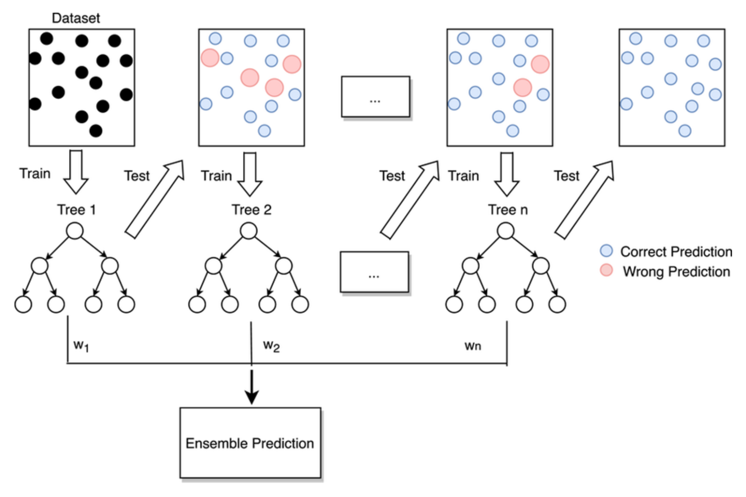
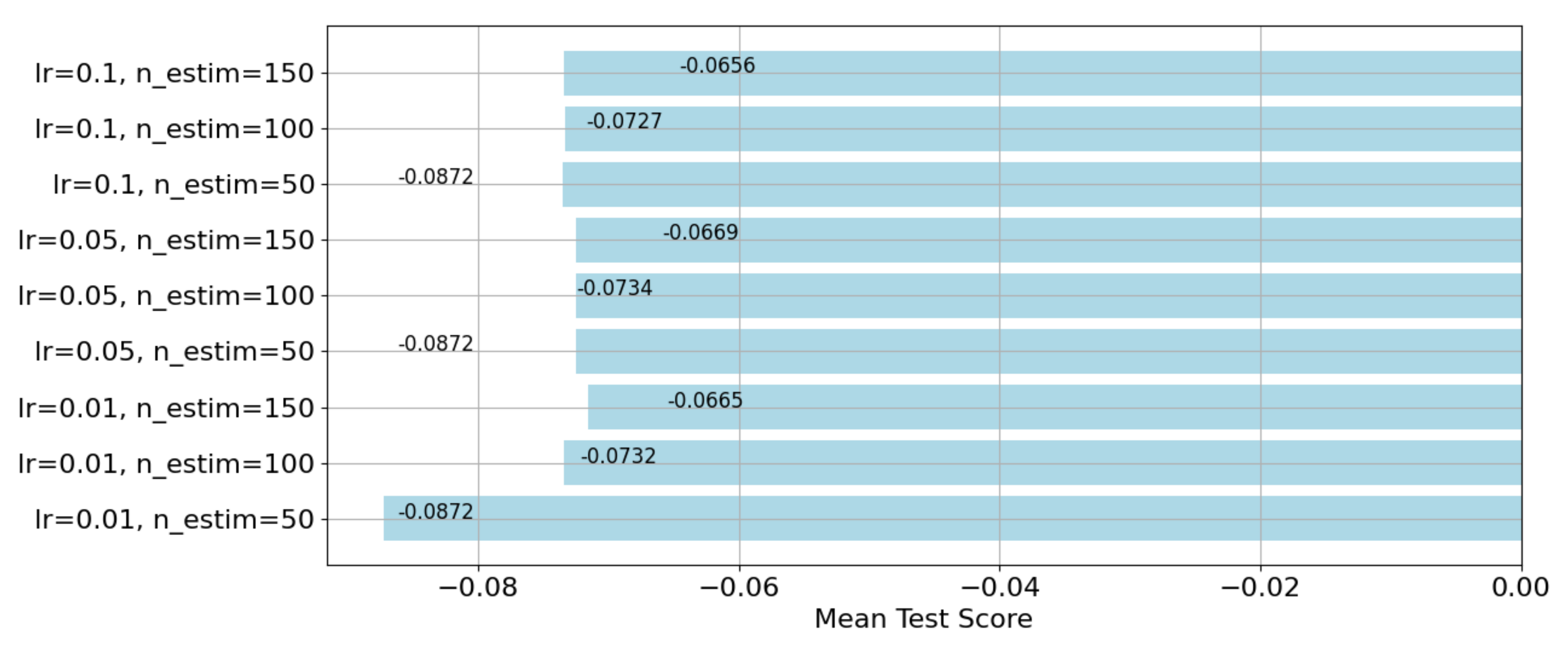
4.1. Run-Up Distance Prediction Based on Gradient Boosting Regression (GBR)

Gradient-Boosting Regressor (GBR) learns an additive, tree-based mapping from the four dimensionless inputs including the relative wave amplitude A, relative wavelength L, Froude number $\mathrm{Fr}$, and relative distance to the seawall D to the target variable relative wave run-up distance on seawall R. See Section 3 for the details of choosing input predictors. Figure 4 illustrates the principle of gradient boosting regression (GBR) model [47].

According to Equation (3), the dataset can be written as:

$${\left\{({\mathbf{x}}_i,R_i)\right\}}_{i=1}^N,\mathrm{with}{\mathbf{x}}_i=(A_i,L_i,{\mathrm{Fr}}_i,D_i)$$

(4)

with ${\mathbf{x}}_i$ the vector of input variables of $i$-th experimental test. There are $N$-th tests in total. Training begins by choosing the constant predictor that minimises the total squared error, namely the sample mean

$$F_0\left(\mathbf{x}\right)=c_0={\displaystyle \frac{1}{N}}\sum _{i=1}^N{R}_i$$

(5)

where $F_0\left(\mathbf{x}\right)$ denotes the average run-up distance for every wave case, which is the starting baseline that later trees will refine. The algorithm then builds the final model:

$$F_M\left(\mathbf{x}\right)=c_0+\sum _{m=1}^M\nu h_m\left(\mathbf{x}\right)$$

(6)

where $F_M\left(\mathbf{x}\right)$ ensemble prediction after integrating the first m-th trees; $h_m\left(\mathbf{x}\right)$ is the shallow decision tree built at stage m, which maps the 4 inputs to a constant within each leaf region; $\nu$ denotes the learning-rate factor, which controls how much influence each new tree adds. Trees are added sequentially. At the m-th step the current residuals $r_{im}$ are treated as a new response variable:

$$r_{im}=R_i-F_{m-1}\left({\mathbf{x}}_i\right)(i=1,\dots ,N)$$

(7)

where the CART tree $h_m$ is fitted by least squares to the pairs $({\mathbf{x}}_i,r_{im})$. Each tree partitions the four dimensional predictor space into disjoint terminal regions $\left\{R_{jm}\right\}$. Within a region $R_{jm}$ the tree output is the average residual:

$${\gamma }_{jm}={\displaystyle \frac{{\sum }_{{\mathbf{x}}_i\in R_{jm}}{r}_{im}}{|R_{jm}|}},h_m\left(\mathbf{x}\right)=\sum _j{\gamma }_{jm}{\mathbf{1}}_{\{\mathbf{x}\in R_{jm}\}}$$

(8)

Then, the model can be updated as:

$$F_m\left(\mathbf{x}\right)=F_{m-1}\left(\mathbf{x}\right)+\nu h_m\left(\mathbf{x}\right)$$

(9)

after which new residuals are computed and another tree is grown. Because each successive tree is trained to explain what its predecessors still miss, the ensemble gradually reduces the overall loss function

$$\mathcal{L}=\sum _{i=1}^N{\left(R_i-F_M\left({\mathbf{x}}_i\right)\right)}^2$$

(10)

with $\mathcal{L}$ the sum of squared differences between predicted and measured relative run-up distance. For an unseen laboratory test $(A^{*},L^{*},{\mathrm{Fr}}^{*},D^{*})$, the predicted run-up distance is obtained by routing the point through every tree to collect the appropriate leaf values and summing them:

$${\widehat{R}}^{*}=c_0+\nu \sum _{m=1}^M{h}_m(A^{*},L^{*},{\mathrm{Fr}}^{*},D^{*})$$

(11)

with $R^{*}$ the relative run-up distance of the unseen laboratory text.

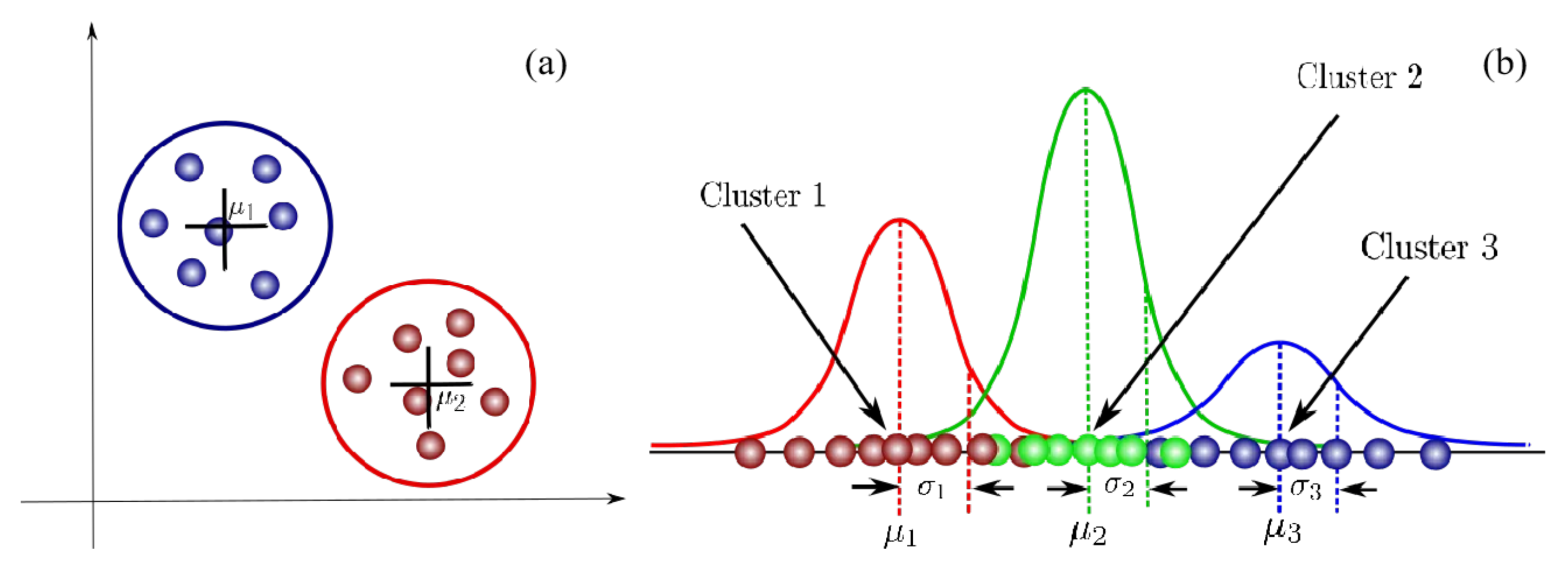
4.2. Data Clustering Using Gaussian Mixture Model (GMM)

Free-surface evolution varies markedly between wave forms. For example, a bore wave exhibits a much steeper rise-and-fall in amplitude than a solitary wave. Such contrasts inject substantial uncertainty into predictive models because the governing dynamics change with the wave type. To reduce this variability we apply a Gaussian Mixture Model (GMM), clustering the experimental records into internally consistent subsets that each represent a single wave class [48]. As shown in Figure 5, GMM treats the data as a superposition of Gaussian distributions, with each component corresponding to one cluster. For the multivariate continuous variables in our study, every component is characterised by its own multivariate normal density.

We cluster the experimental data based on three features: the Froude number $\mathrm{Fr}$, the steepness ratio $A/L$, and the relative distance from the wave to seawall D. $\mathrm{Fr}$ reflects the balance between inertial and gravitational forces, $A/L$ encapsulates the wave’s shape and potential for breaking, and D represents how much momentum can be transferred to the structure as the wave approaches. The GMM treats the wave-characteristic vector:

$$\mathbf{x}={(\mathrm{Fr},A/L,D)}^{\top }$$

(12)

as a random draw from a finite mixture of K multivariate normal populations. Then, the probability density is:

$$p\left(\mathbf{x}\right|\mathsf{\theta })=\sum _{k=1}^K{\pi }_k\mathcal{N}\left(\mathbf{x};{\mathit{\mu }}_k,{\mathsf{\Sigma }}_k\right),\mathcal{N}(\mathbf{x};\mathit{\mu },\mathsf{\Sigma })={\displaystyle \frac{exp\left[-\frac{1}{2}{(\mathbf{x}-\mathit{\mu })}^{\top }{\mathsf{\Sigma }}^{-1}(\mathbf{x}-\mathit{\mu })\right]}{{\left(2\pi \right)}^{3/2}{\left|\mathsf{\Sigma }\right|}^{1/2}}}$$

(13)

where ${\pi }_k\ge 0,{\sum }_k{\pi }_k=1$ are the mixing proportions, ${\mathit{\mu }}_k\in {\mathbb{R}}^3$ is component means and ${\mathsf{\Sigma }}_k\in {\mathbb{R}}^{3\times 3}$ is the positive-definite covariance matrices. The full parameter set is $\mathsf{\theta }={\{{\pi }_k,{\mathit{\mu }}_k,{\mathsf{\Sigma }}_k\}}_{k=1}^K$. Given an experimental sample ${\left\{{\mathbf{x}}_i\right\}}_{i=1}^N$ the parameters are estimated by maximising the log-likelihood function:

$$\ell \left(\mathsf{\theta }\right)=\sum _{i=1}^{N}log\left[\sum _{k=1}^K{\pi }_k\mathcal{N}({\mathbf{x}}_i;{\mathsf{\mu }}_k,{\mathsf{\Sigma }}_k)\right]$$

(14)

which is accomplished with the Expectation-Maximisation (E-M) algorithm, which introduces latent membership indicators $z_{ik}\in \{0,1\}$ (with ${\sum }_k{z}_{ik}=1$) and alternates E-step (posterior responsibilities):

$${\gamma }_{ik}=P(z_{ik}=1|{\mathbf{x}}_i,{\mathsf{\theta }}^{\mathrm{old}})={\displaystyle \frac{{\pi }_k^{\mathrm{old}}\mathcal{N}({\mathbf{x}}_i;{\mathsf{\mu }}_k^{\mathrm{old}},{\mathsf{\Sigma }}_k^{\mathrm{old}})}{{\sum }_{j=1}^K{\pi }_j^{\mathrm{old}}\mathcal{N}({\mathbf{x}}_i;{\mathsf{\mu }}_j^{\mathrm{old}},{\mathsf{\Sigma }}_j^{\mathrm{old}})}};$$

(15)

and M-step (closed-form parameter updates):

$$N_k=\sum _{i=1}^N{\gamma }_{ik},{\pi }_k={\displaystyle \frac{N_k}{N}},{\mathsf{\mu }}_k={\displaystyle \frac{1}{N_k}}\sum _{i=1}^N{\gamma }_{ik}{\mathbf{x}}_i,{\mathsf{\Sigma }}_k={\displaystyle \frac{1}{N_k}}\sum _{i=1}^N{\gamma }_{ik}({\mathbf{x}}_i-{\mathsf{\mu }}_k){({\mathbf{x}}_i-{\mathsf{\mu }}_k)}^{\top }$$

(16)

These two steps monotonically increase $\ell \left(\mathsf{\theta }\right)$ until convergence. Afterward each observation is assigned to the cluster with the largest responsibility to preserve interpretability of the cluster-specific regression models and to reduce computational complexity:

$$\widehat{k}\left({\mathbf{x}}_i\right)=arg\underset{k}{max}{\gamma }_{ik}$$

(17)

In preliminary tests, we compared this hard assignment against soft-probability averaging—where the final prediction is computed as ${\widehat{y}}_i={\sum }_{k=1}^K{\gamma }_{ik}{f}_k\left({\mathbf{x}}_i\right)$ with $f_k$ denoting the GBR model for each cluster.

5. Results

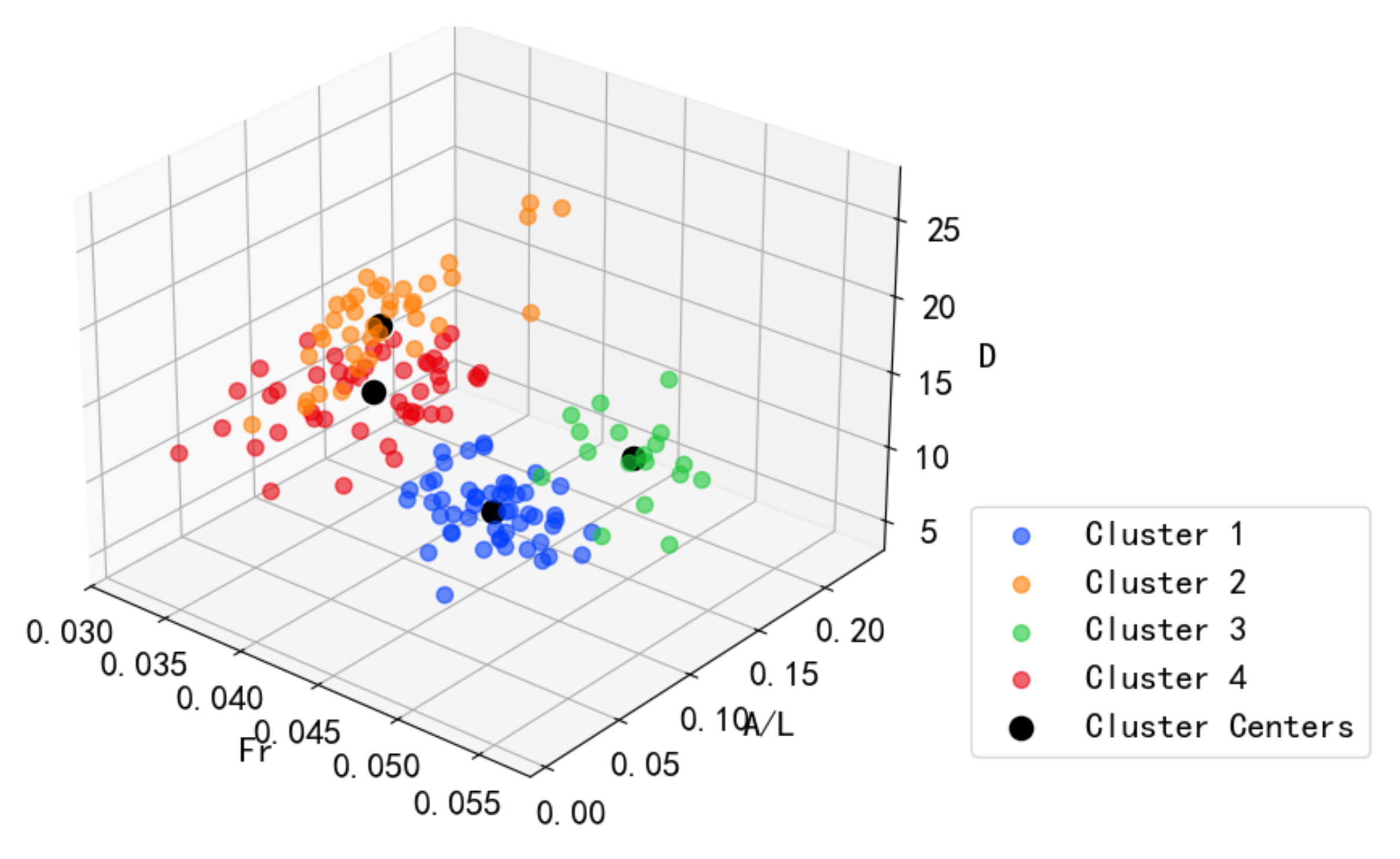
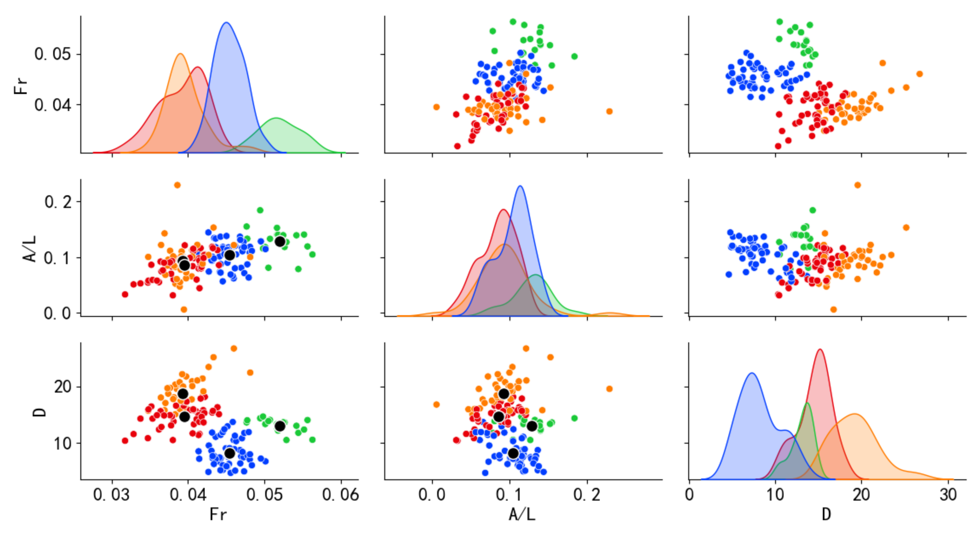
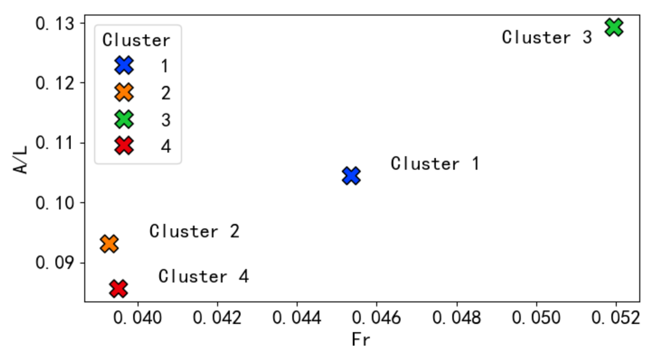
5.1. Clustering Results Using GMM

To categorize the dataset based on wave characteristics, we employed a Gaussian mixture model (GMM) to perform clustering. See Section 4.2 for the detailed mathematical details of the GMM model. The clustering criteria comprised three key variables: the Froude number Fr, which represents wave propagation velocity; the ratio of relative amplitude A to relative wavelength L, serving as an indicator of wave nonlinearity; and the relative distance D from the shoreline. By integrating these parameters, the GMM effectively identified distinct clusters within the dataset, allowing for the differentiation of wave behaviors according to their velocity, nonlinearity, and proximity to the shoreline. This classification ensures that each cluster encapsulates homogeneous wave characteristics.

Figure 6 presents a three-dimensional scatter plot illustrating the clustering results obtained using the GMM. The plot visualizes data points across three features: Fr, $A/L$, and D, with each point colored according to its assigned cluster. The dataset is separated into 4 different clusters. The cluster centers are marked with black circular markers, representing the mean positions of each cluster in the original feature space. The coordinates of the cluster centers are summarized as follows: Cluster 1: Fr = 0.0454, $A/L$ = 0.1044, D = 8.2037; Cluster 2: Fr = 0.0393, $A/L$ = 0.0931, D = 18.6823; Cluster 3: Fr = 0.0520, $A/L$ = 0.1292, D = 13.0564; Cluster 4: Fr = 0.0395, $A/L$ = 0.0856, D = 14.7375. Of the 156 experiments, Cluster 1 contains 56 tests, Cluster 2 contains 31, Cluster 3 contains 17, and Cluster 4 contains 52.

Figure 7 showcases a pairwise scatter plot matrix, commonly known as a PairGrid, which explores the relationships between the three features Fr, $A/L$, and D. Each subplot within the matrix displays a scatter plot for a unique pair of features, with data points colored based on their cluster assignments. The diagonal subplots feature kernel density estimates, providing insights into the distribution of individual features. This detailed pairwise analysis complements the GMM’s probabilistic approach by revealing how clusters are distributed and overlap across different feature dimensions, highlighting the nuanced separations that GMM effectively captures through its mixture of Gaussian distributions. By projecting the cluster centers onto a specific two-feature plane, this plot underscores how GMM leverages the underlying Gaussian distributions to determine the optimal placement of cluster centers, ensuring that each cluster is well-represented within the feature space. The 4 clusters are clearly separated in each dimension, indicating distinct groupings based on wave propagation velocity, wave nonlinearity, and proximity to the shoreline. The clear separation of clusters across all feature dimensions validates the efficacy of the GMM in capturing the inherent structure of the data.

Figure 8 provides on a two-dimensional scatter plot that highlights the positions of cluster centers within the Fr versus $A/L$ feature space. Each cluster center is represented by a black X marker. The plot emphasizes the spatial distribution of cluster centers, allowing for a focused analysis of their relationships and separations within these two features. The corresponding coordinates at (Fr, $A/L$ space for cluster 1 to 4 are (0.0454, 0.1044), (0.0393, 0.0931), (0.0520, 0.129)2, (0.0395, 0.0856), respectively.

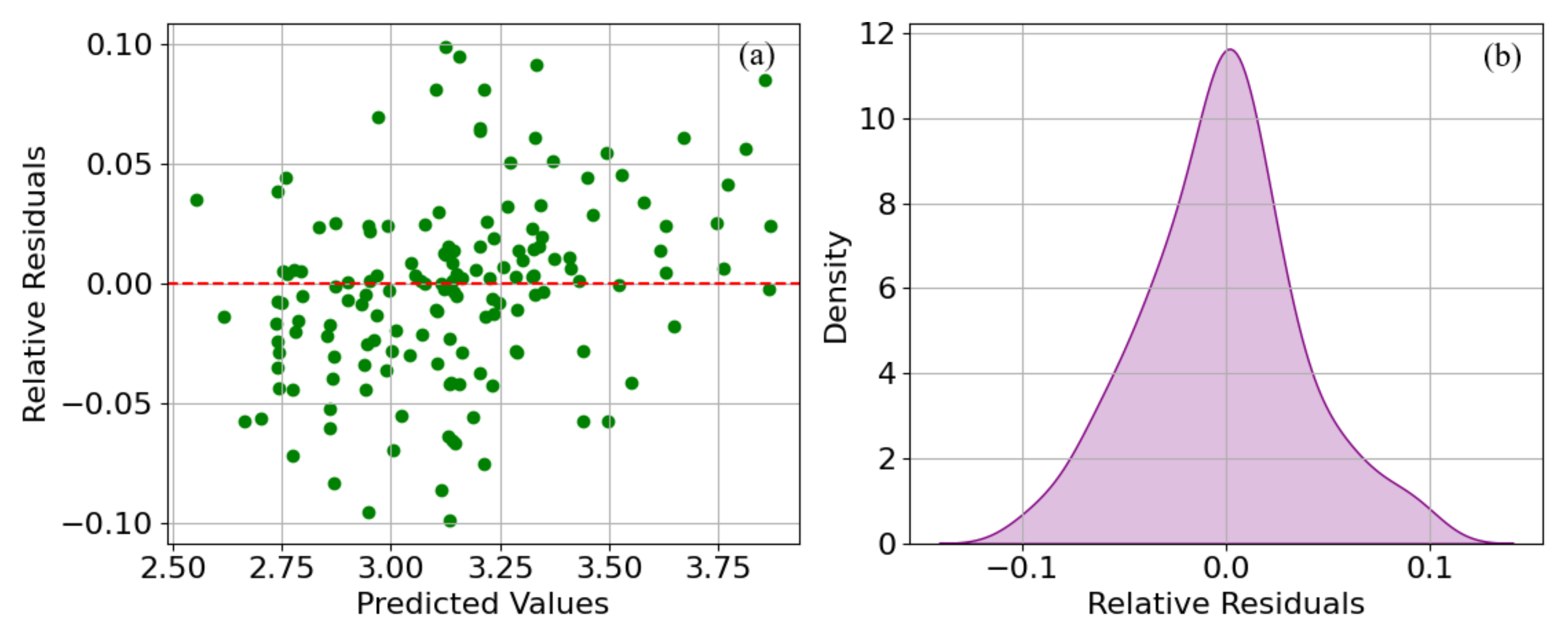
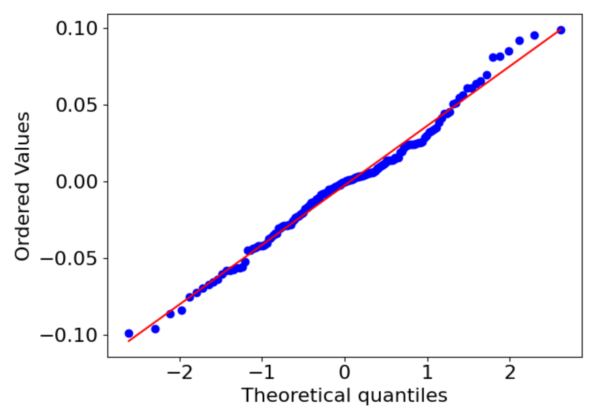
5.2. Predicting Results

Prior to clustering, the dataset was standardized to ensure that all explanatory variables contribute equally to the analysis, thereby mitigating the effects of differing scales. The original input values exhibited significant variability: relative distance D mainly ranged from 10 to 15, Froude number Fr mainly from 0.02 to 0.06, relative amplitude A from 0.5 to 1.0, and relative wavelength L from 5 to 15. To address this, each variable was transformed to a standardized scale between −1 and 1 using min-max scaling, facilitating a more balanced comparison and enhancing the performance of the prediction model based on Gradient Boosting Regression (GBR). Figure 9 illustrates the distribution of data before and after standardization, highlighting the uniform scaling achieved across all four parameters.

A comprehensive hyperparameter tuning process was undertaken to optimize the performance of the Gradient Boosting Regression (GBR) model. Utilizing GridSearchCV with 5-fold cross-validation, a total of 243 hyperparameter combinations were evaluated, resulting in 1215 individual model fits. This extensive search aimed to identify the most effective set of parameters for enhancing the model’s predictive accuracy and generalizability. Figure 10 shows the mean test score of several selected cases. The best-performing configuration was determined to include a learning rate $lr$ of 0.05, a maximum depth of 3, minimum samples per leaf set to 4, minimum samples required to split an internal node set to 10, and 100 estimators. These optimal parameters balance the trade-off between model complexity and performance, ensuring robust predictions while mitigating the risk of overfitting. The selected hyperparameters is utilized in subsequent analyses to provide reliable and accurate forecasting results.

Figure 11 compares the actual data with predicted data. It can be seen from the figure that predicted data fit fairly well with actual data, indicating that the model effectively captures the underlying data distribution.

As shown in Figure 12, the relative residuals $\sigma$ are randomly distributed around the zero line, ranging between −0.5 and 0.5. This distribution indicates that there are no significant patterns or biases in the model’s predictions, suggesting that the model effectively captures the underlying relationships within the data without introducing systematic errors. Additionally, the $\sigma$ follow a normal distribution, further validating the model’s performance. The randomness and normality of $\sigma$ imply that the model’s predictions are both unbiased and reliable.

Figure 13 illustrates the feature importance of the four input parameters utilized in the GBR model. Among these, the relative distance D emerges as the most influential factor, with an importance score of 0.443, indicating its substantial role in predicting the target variable. This is followed by the relative amplitude A with an importance score of 0.230, highlighting its significant contribution to the model’s predictive capabilities. The relative wavelength L holds an importance score of 0.194, suggesting a moderate influence on the predictions. Lastly, the Froude number $Fr$ exhibits the lowest importance score of 0.133, indicating that it plays a lesser role compared to the other variables in the model. These results imply that proximity to the shoreline D is the most critical factor affecting the model’s performance, possibly due to its direct impact on wave dynamics. Evaluating the relative importance of the input variables clarifies the underlying processes represented by the model.

Figure 14 displays the results of normality test for relative residual $\sigma$. As illustrated in the figure, data points closely adhere to the reference line, indicating that the residuals are approximately normally distributed. It support the robustness of the model and its suitability for forecasting tasks within the studied domain.

Metrics including Mean Squared Error MSE, Mean Absolute Error MAE, and coefficient of determination $R^2$ are used to quantify the evaluation of model. High $R^2$ reflects a high level of predictive power. The low MSE and MAE values indicate minimal prediction errors, underscoring the model’s precision and reliability.

Table 1. Comparison of the evaluation metrics of the proposed GMM-GBR model with the GBR model.

${\mathit{R}}^2$	GMM-GBR Model	GBR Model
MAE	0.07	0.09
MSE	0.012	0.015
R2	0.91	0.86

provides the evaluation metrics of the proposed GMM-GBR Model against the conventional GBR Model. The $R^2$ of the proposed model and conventional GBR model are 0.91 and 0.86, respectively. The comparison confirms that the proposed GMM-GBR model outperforms the conventional GBR model.

6. Conclusions

This study combines physical experiments with machine-learning techniques to predict wave run-up distance on seawall. Two-dimensional tests were carried out in a narrow flume, and four dimensionless parameters were extracted as explanatory variables: relative shoreline distance D, relative wave amplitude A, relative wavelength L, and the Froude number Fr. The resulting data were first classified into four clusters with a Gaussian Mixture Model (GMM) using Fr, D, and $A/L$ as features. Within each cluster, a Gradient Boosting Regressor (GBR) was trained to estimate the relative run-up distance on seawall $R_m$. The hybrid GMM-GBR framework attained an $R^2$ of 0.91 and an MSE of 0.015, surpassing a conventional non-clustered GBR ($R^2=0.86$). These results highlight the model’s high prediction accuracy. Feature-importance analysis showed that D exerted the strongest influence on $R_m$, followed, in order, by A, L, and Fr. The principal advantage of the proposed GMM–GBR framework is its ability to isolate hydrodynamically distinct regimes before fitting a nonlinear regressor to each regime, yielding higher predictive accuracy than a single global model.

The proposed model still face several limitations. First, the water flume used in the experiments was not sufficiently long, which may have constrained the length of wave propagation. A longer flume could provide a more representative environment for wave interactions. In addition, while the present hybrid GMM–GBR model was developed and evaluated using controlled laboratory flume data, its applicability to field scale conditions remains to be established. In future studies, we will extend the hybrid GMM–GBR framework by incorporating extensive field monitoring data such as full scale run-up and overtopping measurements from coastal observatories to both train and validate the model. By using real world wave and water level records to define clusters and fit the regression models, we aim to adapt the methodology to fully irregular sea states and site-specific bathymetries, ensuring robust predictive performance under operational field conditions.

References

1. Koraim, A.; Heikal, E.; Zaid, A.A. Hydrodynamic characteristics of porous seawall protected by submerged breakwater. Appl. Ocean Res. 2014, 46, 1–14. [Google Scholar] [CrossRef]
2. Mase, H.; Miyahira, A.; Hedges, T.S. Random wave runup on seawalls near shorelines with and without artificial reefs. Coast. Eng. J. 2004, 46, 247–268. [Google Scholar] [CrossRef]
3. Liu, X.; Li, X.; Ma, G.; Rezania, M. Characterization of spatially varying soil properties using an innovative constraint seed method. Comput. Geotech. 2025, 183, 107184. [Google Scholar] [CrossRef]
4. Zhang, J.; Zhang, X.; Li, H.; Fan, Y.; Meng, Z.; Liu, D.; Pan, S. Optimization of Water Quantity Allocation in Multi-Source Urban Water Supply Systems Using Graph Theory. Water 2025, 17, 61. [Google Scholar] [CrossRef]
5. Gao, J.; Ma, X.; Zang, J.; Dong, G.; Ma, X.; Zhu, Y.; Zhou, L. Numerical investigation of harbor oscillations induced by focused transient wave groups. Coast. Eng. 2020, 158, 103670. [Google Scholar] [CrossRef]
6. Meng, Z.; Zhang, J.; Hu, Y.; Ancey, C. Temporal Prediction of Landslide-Generated Waves Using a Theoretical-Statistical Combined Method. J. Mar. Sci. Eng. 2023, 11, 1151. [Google Scholar] [CrossRef]
7. Ebrahimi, A.; Askar, M.B.; Pour, S.H.; Chegini, V. Investigation of various random wave run-up amounts under the influence of different slopes and roughnesses. Environ. Conserv. J. 2015, 16, 301–308. [Google Scholar] [CrossRef]
8. Gao, J.; Hou, L.; Liu, Y.; Shi, H. Influences of bragg reflection on harbor resonance triggered by irregular wave groups. Ocean Eng. 2024, 305, 117941. [Google Scholar] [CrossRef]
9. Meng, Z.; Wang, Y.; Zheng, S.; Wang, X.; Liu, D.; Zhang, J.; Shao, Y. Abnormal Monitoring Data Detection Based on Matrix Manipulation and the Cuckoo Search Algorithm. Mathematics 2024, 12, 1345. [Google Scholar] [CrossRef]
10. Sujantoko, S.; Fuad, H.F.; Azzarine, S.; Raehana, D.R. Experimental Study of Wave Run-Up for Porous Concrete on Seawall Structures. E3S Web Conf. 2024, 576, 02004. [Google Scholar] [CrossRef]
11. McCabe, M.; Stansby, P.K.; Apsley, D.D. Random wave runup and overtopping a steep sea wall: Shallow-water and Boussinesq modelling with generalised breaking and wall impact algorithms validated against laboratory and field measurements. Coast. Eng. 2013, 74, 33–49. [Google Scholar] [CrossRef]
12. Ting-Chieh, L.; Hwang, K.S.; Hsiao, S.C.; Ray-Yeng, Y. An experimental observation of a solitary wave impingement, run-up and overtopping on a seawall. J. Hydrodyn. Ser. B 2012, 24, 76–85. [Google Scholar]
13. Gao, J.; Ma, X.; Dong, G.; Chen, H.; Liu, Q.; Zang, J. Investigation on the effects of Bragg reflection on harbor oscillations. Coast. Eng. 2021, 170, 103977. [Google Scholar] [CrossRef]
14. Neelamani, S.; Sandhya, N. Surface roughness effect of vertical and sloped seawalls in incident random wave fields. Ocean Eng. 2005, 32, 395–416. [Google Scholar] [CrossRef]
15. Neelamani, S.; Schüttrumpf, H.; Muttray, M.; Oumeraci, H. Prediction of wave pressures on smooth impermeable seawalls. Ocean Eng. 1999, 26, 739–765. [Google Scholar] [CrossRef]
16. Larson, M.; Erikson, L.; Hanson, H. An analytical model to predict dune erosion due to wave impact. Coast. Eng. 2004, 51, 675–696. [Google Scholar] [CrossRef]
17. Gao, J.; Shi, H.; Zang, J.; Liu, Y. Mechanism analysis on the mitigation of harbor resonance by periodic undulating topography. Ocean Eng. 2023, 281, 114923. [Google Scholar] [CrossRef]
18. Liu, X.; Jiang, S.H.; Xie, J.; Li, X. Bayesian inverse analysis with field observation for slope failure mechanism and reliability assessment under rainfall accounting for nonstationary characteristics of soil properties. Soils Found. 2025, 65, 101568. [Google Scholar] [CrossRef]
19. Di Leo, A.; Dentale, F.; Buccino, M.; Tuozzo, S.; Pugliese Carratelli, E. Numerical analysis of wind effect on wave overtopping on a vertical seawall. Water 2022, 14, 3891. [Google Scholar] [CrossRef]
20. Schwab, D.J.; Bennett, J.R.; Liu, P.C.; Donelan, M.A. Application of a simple numerical wave prediction model to Lake Erie. J. Geophys. Res. Ocean. 1984, 89, 3586–3592. [Google Scholar] [CrossRef]
21. Wu, G.K.; Li, R.Y.; Li, D.W. Research on numerical modeling of two-dimensional freak waves and prediction of freak wave heights based on LSTM deep learning networks. Ocean Eng. 2024, 311, 119032. [Google Scholar] [CrossRef]
22. Huang, C.J.; Chang, Y.C.; Tai, S.C.; Lin, C.Y.; Lin, Y.P.; Fan, Y.M.; Chiu, C.M.; Wu, L.C. Operational monitoring and forecasting of wave run-up on seawalls. Coast. Eng. 2020, 161, 103750. [Google Scholar] [CrossRef]
23. Buccino, M.; Di Leo, A.; Tuozzo, S.; Lopez, L.F.C.; Calabrese, M.; Dentale, F. Wave overtopping of a vertical seawall in a surf zone: A joint analysis of numerical and laboratory data. Ocean Eng. 2023, 288, 116144. [Google Scholar] [CrossRef]
24. Amini, E.; Marsooli, R.; Ayyub, B.M. Assessing Beach–Seawall Hybrid Systems: A Novel Metric-Based Approach for Robustness and Serviceability. Asce-Asme J. Risk Uncertain. Eng. Syst. Part Civ. Eng. 2024, 10, 04023062. [Google Scholar] [CrossRef]
25. Zhang, J.; Benoit, M.; Kimmoun, O.; Chabchoub, A.; Hsu, H.C. Statistics of extreme waves in coastal waters: Large scale experiments and advanced numerical simulations. Fluids 2019, 4, 99. [Google Scholar] [CrossRef]
26. Rasmeemasmuang, T.; Rattanapitikon, W. Predictions of run-up scale on coastal seawalls using a statistical formula. J. Ocean Eng. Mar. Energy 2021, 7, 173–187. [Google Scholar] [CrossRef]
27. Cao, D.; Yuan, J.; Chen, H.; Zhao, K.; Liu, P.L.F. Wave overtopping flow striking a human body on the crest of an impermeable sloped seawall. Part I: Physical modeling. Coast. Eng. 2021, 167, 103891. [Google Scholar] [CrossRef]
28. Salauddin, M.; Shaffrey, D.; Habib, M. Data-driven approaches in predicting scour depths at a vertical seawall on a permeable shingle foreshore. J. Coast. Conserv. 2023, 27, 18. [Google Scholar] [CrossRef]
29. Chen, H.; Huang, S.; Xu, Y.P.; Teegavarapu, R.S.; Guo, Y.; Nie, H.; Xie, H. Using baseflow ensembles for hydrologic hysteresis characterization in humid basins of Southeastern China. Water Resour. Res. 2024, 60, e2023WR036195. [Google Scholar] [CrossRef]
30. Beuzen, T.; Goldstein, E.B.; Splinter, K.D. Ensemble models from machine learning: An example of wave runup and coastal dune erosion. Nat. Hazards Earth Syst. Sci. 2019, 19, 2295–2309. [Google Scholar] [CrossRef]
31. Berbić, J.; Ocvirk, E.; Carević, D.; Lončar, G. Application of neural networks and support vector machine for significant wave height prediction. Oceanologia 2017, 59, 331–349. [Google Scholar] [CrossRef]
32. Chen, H.; Xu, B.; Qiu, H.; Huang, S.; Teegavarapu, R.S.; Xu, Y.P.; Guo, Y.; Nie, H.; Xie, H. Adaptive assessment of reservoir scheduling to hydrometeorological comprehensive dry and wet condition evolution in a multi-reservoir region of southeastern China. J. Hydrol. 2025, 648, 132392. [Google Scholar] [CrossRef]
33. Li, J.; Meng, Z.; Zhang, J.; Chen, Y.; Yao, J.; Li, X.; Qin, P.; Liu, X.; Cheng, C. Prediction of Seawater Intrusion Run-Up Distance Based on K-Means Clustering and ANN Model. J. Mar. Sci. Eng. 2025, 13, 377. [Google Scholar] [CrossRef]
34. Habib, M.; O’Sullivan, J.; Abolfathi, S.; Salauddin, M. Enhanced wave overtopping simulation at vertical breakwaters using machine learning algorithms. PLoS ONE 2023, 18, e0289318. [Google Scholar] [CrossRef]
35. Liu, Y.; Li, S.; Zhao, X.; Hu, C.; Fan, Z.; Chen, S. Artificial neural network prediction of overtopping rate for impermeable vertical seawalls on coral reefs. J. Waterw. Port Coast. Ocean Eng. 2020, 146, 04020015. [Google Scholar] [CrossRef]
36. Vileti, V.L.; Ersdal, S. Wave Dynamics Run-Up Modelling: Machine Learning Approach. In Proceedings of the International Conference on Offshore Mechanics and Arctic Engineering. Am. Soc. Mech. Eng. 2024, 87837, V05BT06A072. [Google Scholar]
37. Savitha, R.; Al Mamun, A. Regional ocean wave height prediction using sequential learning neural networks. Ocean Eng. 2017, 129, 605–612. [Google Scholar]
38. Stansberg, C.T.; Baarholm, R.; Berget, K.; Phadke, A.C. Prediction of wave impact in extreme weather. In Proceedings of the Offshore Technology Conference. OTC, Houston, TX, USA, 3–6 May 2010; p. OTC-20573. [Google Scholar]
39. Belmont, M.; Horwood, J.; Thurley, R.; Baker, J. Filters for linear sea-wave prediction. Ocean Eng. 2006, 33, 2332–2351. [Google Scholar] [CrossRef]
40. Reynolds, D.A. Gaussian mixture models. Encycl. Biom. 2009, 741, 827–832. [Google Scholar]
41. Biau, G.; Cadre, B.; Rouvìère, L. Accelerated gradient boosting. Mach. Learn. 2019, 108, 971–992. [Google Scholar] [CrossRef]
42. Meng, Z.; Hu, Y.; Jiang, S.; Zheng, S.; Zhang, J.; Yuan, Z.; Yao, S. Slope Deformation Prediction Combining Particle Swarm Optimization-Based Fractional-Order Grey Model and K-Means Clustering. Fractal Fract. 2025, 9, 210. [Google Scholar] [CrossRef]
43. Saha, S.; De, S.; Changdar, S. An application of machine learning algorithms on the prediction of the damage level of rubble-mound breakwaters. J. Offshore Mech. Arct. Eng. 2024, 146, 011202. [Google Scholar] [CrossRef]
44. Scala, P.; Manno, G.; Ingrassia, E.; Ciraolo, G. Combining Conv-LSTM and wind-wave data for enhanced sea wave forecasting in the Mediterranean Sea. Ocean Eng. 2025, 326, 120917. [Google Scholar] [CrossRef]
45. Kim, T.; Kwon, S.; Kwon, Y. Prediction of wave transmission characteristics of low-crested structures with comprehensive analysis of machine learning. Sensors 2021, 21, 8192. [Google Scholar] [CrossRef]
46. Maugis, C.; Celeux, G.; Martin-Magniette, M.L. Variable selection for clustering with Gaussian mixture models. Biometrics 2009, 65, 701–709. [Google Scholar] [CrossRef]
47. Natekin, A.; Knoll, A. Gradient boosting machines, a tutorial. Front. Neurorobot. 2013, 7, 21. [Google Scholar] [CrossRef]
48. Huang, T.; Peng, H.; Zhang, K. Model selection for Gaussian mixture models. Stat. Sin. 2017, 27, 147–169. [Google Scholar] [CrossRef]
Figure 1. The diagram of experiments: (a) seawall, (b) wave run-up on seawall, (c) flume, (d) stage I of the impacting process, and (e) stage II of the impacting process.
Jmse 13 01298 g001
Figure 2. The correlation matrix between each explanatory variables.
Jmse 13 01298 g002
Figure 3. The (a) frequency distribution, (b) KDE and (c) box distribution of D; The (d) frequency distribution, (e) KDE and (f) box distribution of Fr; The (g) frequency distribution, (h) KDE and (i) box distribution of A; The (j) frequency distribution, (k) KDE and (l) box distribution of L.
Jmse 13 01298 g003
Figure 4. The principle of GBR model.
Jmse 13 01298 g004
Figure 5. (a) Two clusters with their respective centroids marked; (b) Diagram illustrating each cluster’s mean μ and standard deviation σ .
Jmse 13 01298 g005
Figure 6. Three dimensional plot of the clustering results and cluster centres.
Jmse 13 01298 g006
Figure 7. Feature pairwise scatter plot with cluster center annotations.
Jmse 13 01298 g007
Figure 8. Cluster centers of the 4 clusters in Fr and A / L space.
Jmse 13 01298 g008
Figure 9. The standardization of dataset: (a) before standardization and (b) after standardization.
Jmse 13 01298 g009
Figure 10. Cross validation performance for different hyperparameters.
Jmse 13 01298 g010
Figure 11. Comparison of the actual data with the predicted data.
Jmse 13 01298 g011
Figure 12. The (a) distribution and (b) PDF of relative residual σ .
Jmse 13 01298 g012
Figure 13. The feature importance of the input parameters.
Jmse 13 01298 g013
Figure 14. The normality distribution of relative residual σ .
Jmse 13 01298 g014