CFD-Based Parameter Calibration and Design of Subwater In Situ Cultivation Chambers Toward Well-Mixing Status but No Sediment Resuspension

Abstract

The elemental exchange fluxes at the sediment–water interface play a crucial role in Earth’s climate regulation, environmental change, and ecosystem dynamics. Accurate in situ measurements of these fluxes depend heavily on the performance of marine incubation devices, particularly their ability to achieve full mixing without causing sediment resuspension. This study presents a novel parameter calibration method for a marine in situ incubation device using a combination of computational fluid dynamics (CFD) simulations and laboratory experiments. The influence of the stirring paddle’s rotational speed on flow field distribution, complete mixing time, and sediment resus-pension was systematically analyzed. The CFD simulation results were validated against existing device data and actual experimental measurements. The deviation in complete mixing time between simulation and experiment was within −9.23% to 9.25% for 20 cm of sediment and −9.4% to 9.1% for 15 cm. The resuspension tests determined that optimal mixing without sediment disturbance occurs at rotational speeds of 25 r/min and 35 r/min for the two sediment depths, respectively. Further analysis showed that the stirring paddle effectively creates a uniform flow field within the chamber. This CFD-based calibration method provides a reliable approach to parameter tuning for various in situ devices by adjusting boundary conditions, offering a scientific foundation for device design and deployment, and introducing a new framework for future calibration efforts.

1. Introduction

As the largest component of Earth’s ecosystem, the marine environment presents significant challenges to scientific research due to its vastness, dynamic conditions, and complex biogeochemical processes. In situ observation devices, serving as essential tools for studying material and elemental exchange at the sediment–water inter-face, hold considerable scientific value. They contribute to understanding global carbon cycle mechanisms, assessing the potential for marine resource utilization, and monitoring ecological systems [1,2,3,4,5]. Quantitative analysis of element exchange rates at the sediment–water interface—referred to as benthic flux—provides essential data support for marine science research [6,7]. However, conventional sampling methods are limited by physical and chemical constraints, particularly the distortion of samples during post-processing. To overcome these limitations, the development of marine in situ incubation technology has emerged as a viable solution.

Since 1968, efforts to develop in situ incubation devices have been ongoing. Notable examples include the “Benvir” deep-sea boundary layer monitoring device (2010) [8], the adaptive stirring-rate benthic flux instrument developed by Zhejiang University (2017) [9], and the GÖTEBORG 2 system developed by the University of Gothenburg (2020) [6]. With technological advancement, in situ devices have evolved from bulky, shallow-sea operations to more compact, intelligent systems capable of operating in diverse marine environments. The design of such devices must meet specific functional requirements, including precise parameter settings within the chamber to ensure the effectiveness of the incubation process [8]. Traditional parameter calibration methods, such as those by Tengberg—based on visual mixing time, diffusion boundary layer (DBL) sensor testing, and resuspension observation—suggest that optimal in situ incubation depends on two key factors: sufficient mixing of overlying water and the avoidance of sediment resuspension [10]. Addressing these challenges is essential for obtaining reliable in situ benthic flux measurements. This study focuses on analyzing flow field variations induced by impeller rotation and experimentally verifying its impact on sediment resuspension within the chamber.

To improve parameter calibration accuracy, this study proposes a method that integrates CFD simulations with laboratory experiments to investigate the internal flow characteristics of the incubation chamber [11]. CFD simulations provide detailed insights into complex fluid dynamics, which are crucial for the design of stirring blades, control system optimization, and overall flow field distribution in the chamber structure [12]. This paper further examines how impeller rotation influences flow field uniformity and sediment resuspension through experimental validation. Accurate numerical simulations are critical for predicting flow behaviors, particularly for determining the time required for full mixing between sediment and overlying water and evaluating flow field uniformity in chambers of varying geometries [9,12,13,14]. Therefore, this study employs CFD-based flow field simulations alongside experimental testing to calibrate and verify the device parameters. The findings not only enhance the reliability of the calibration method and the rationality of the design but also provide important scientific support for the advancement of marine in situ incubation technologies. Additionally, this work offers valuable data for marine resource development and environmental monitoring.

2. Fluid Models and Simulation Strategies

2.1. Transient Tracer Simulation Based on Steady MRF Flow

The commonly used moving reference frame (MRF) model provides results that closely approximate those obtained from sliding mesh simulations at low rotational speeds. In scenarios without a stator, the flow remains steady relative to the rotating components. The MRF model is reliable when the interaction between the rotor and stator is weak, as it approximates the influence of rotating parts through time-averaged values. This model efficiently provides a preliminary flow field—such as pressure distribution and dominant flow directions—without the need for full transient simulation convergence from initial conditions, thereby significantly reducing the computational cost. It is particularly suitable for analyzing rotational or translational motion in steady-state conditions [15,16]. For the steady-state simulation involving only water, the boundary conditions implemented were no-slip walls and rotational wall motion. The computational domain is divided into a rotating zone, where the impeller resides, and a stationary zone representing the tank body. Within each zone, the flow equations are solved in their respective reference frames, and proper interface treatment ensures continuity and momentum transfer between the regions [17]. In the static reference frame, the steady-state incompressible Navier–Stokes equations are solved, specifically the continuity and momentum equations:

$$\nabla ·u=0$$

(1)

$$\rho \left(u·\nabla \right)u=-\nabla p+\nu {\nabla }^{2}u+f$$

(2)

where $u$ is the relative velocity vector; $p$ is the time-averaged pressure field; $\rho$ is the fluid density; and $f$ is the body force due to gravity.

In the rotating frame, in order to account for the relative angular velocity in the MRF zone, Equation (2) is solved with the additional Coriolis and centrifugal terms. With a specific rearrangement of the equation that facilitates the computation, the momentum equation solved in the rotating frame is expressed as follows:

$$\rho \left(\left(u·\nabla \right)u+2\mathsf{\Omega }\times u+\mathsf{\Omega }\times \left(\mathsf{\Omega }\times r\right)\right)=-\nabla p+\mu {\nabla }^{2}u$$

(3)

where $\mathsf{\Omega }$ is the angular velocity vector; $r$ is the position vector from the rotation axis; and $\mu$ is the kinematic viscosity. The Coriolis force is $2\mathsf{\Omega }\times u$ and the centrifugal force is $\mathsf{\Omega }\times \left(\mathsf{\Omega }\times r\right)$.

During the transient stage, the passive scalar (representing the tracer) is modeled using a species transport model without chemical reactions. To simulate a frozen flow field, only the transport equation of phase-water trace is activated during the solution of the governing equations, so that only the concentration evolves over time while the flow field remains unchanged [17,18,19]. The tracer is assumed to have negligible influence on the flow field and thus behaves as a passive scalar. The governing equation includes only convection and diffusion terms. The scalar transport equation for the passive tracer is expressed as follows:

$${\displaystyle \frac{\partial C}{\partial t}}+u·\nabla C=D{\nabla }^{2}C$$

(4)

where $C$ is the concentration of the tracer; $u$ is the velocity vector obtained from the steady-state MRF simulation; and $D$ is the molecular diffusion coefficient (fixed at 1 × 10⁻⁹ m²/s due to the tracer’s physical properties being similar to those of water.

2.2. Multiphase Flow Model

The volume of fluid (VOF) method describes the distribution of each phase using volume fractions ranging from 0 to 1, and its initial conditions must accurately reflect the real physical scenario. The interface between phases is captured by solving the volume fraction transport equation for each phase. In the steady-state simulation, the culture chamber is assumed to be completely filled with seawater, with the water phase volume fraction set to 1 and the air phase set to 0. Based on the actual conditions, the initial flow field is first obtained throughout the simulation domain. This configuration prevents the introduction of unnecessary phase simplification issues in a sealed system. By specifying the surface tension coefficient, it ensures the completeness of the material definitions and the realism of boundary behaviors, thereby enhancing the accuracy of the simulation [16]. In transient simulation, a local area is initialized with tracer (volume fraction of 1), while the volume fractions in other water body areas are set to 0. As time progresses, the volume fraction transport equation is solved through VOF to visualize the mixing process. Accordingly, species transport is defined in the transient calculation. The interface location is determined by computing the spatial volume fraction distribution of each phase [20,21,22]. Moreover, although the VOF model is originally designed to track sharp interfaces between immiscible phases, in this study, it was adapted for visualizing the mixing process by treating the tracer as a secondary phase with an artificially assigned volume fraction. This approach does not capture molecular diffusion, but it effectively illustrates the large-scale distribution and evolution of the mixing contours, offering clearer visualization than traditional scalar transport models in complex flow domains [23,24]. Therefore, this study employs a multiphase flow model based on the VOF method. In the transient simulation, the fluid domain was divided into two immiscible phases, each assigned a unique volume fraction identifier. Their relationship is defined as follows:

$$F_1+F_2=F$$

(5)

This implies that the sum of the volume fractions of the sub-liquid phases is equal to the total liquid phase volume. The evolution of the volume fractions $F_1$ and $F_2$ can be described by the following transport equations:

$${\displaystyle \frac{\partial F_1}{\partial t}}+\overrightarrow{u}\cdot \nabla F_1=0$$

(6)

$${\displaystyle \frac{\partial F_2}{\partial t}}+\overrightarrow{u}\cdot \nabla F_2=0$$

(7)

Equations (6) and (7) can be independently solved using the VOF method. The total volume fraction function can be derived based on the relationship defined in Equation (5), allowing for the reconstruction of both the overall liquid interface and the interfaces between the two individual liquid phases [23].

2.3. Standard $RNGK–\epsilon$ Turbulence Model

This study adopts the standard RNG K–ε turbulence model. which offers improved accuracy for rapidly deforming flows, swirl effects, and transient phenomena. It is widely applicable across various flow conditions and provides more accurate dissipation rate predictions [25,26]. The turbulent kinetic energy and dissipation equations of the standard RNG K–ε turbulence model are as follows:

$${\displaystyle \frac{\partial \left(\rho k\right)}{\partial t}}+{\displaystyle \frac{\partial \left(\rho u_{j}k\right)}{\partial x_j}}={\displaystyle \frac{\partial }{\partial x_j}}\left[\left(\mu +{\displaystyle \frac{{\mu }_t}{\sigma k}}\right){\displaystyle \frac{\partial k}{\partial x_j}}\right]+{\mu }_t\left({\displaystyle \frac{\partial u_i}{\partial x_j}}+{\displaystyle \frac{\partial u_j}{\partial x_i}}\right){\displaystyle \frac{\partial u_i}{\partial x_j}}-\rho \epsilon$$

(8)

$${\displaystyle \frac{\partial \left(\rho \epsilon \right)}{\partial t}}+{\displaystyle \frac{\partial \left(\rho u_j\epsilon \right)}{\partial x_j}}={\displaystyle \frac{\partial }{\partial x_j}}\left[\left(\mu +{\displaystyle \frac{{\mu }_t}{\sigma \epsilon }}\right){\displaystyle \frac{\partial \epsilon }{\partial x_j}}\right]+{C_{\epsilon 1}^{*}{\displaystyle \frac{\epsilon }{k}}\mu }_t\left({\displaystyle \frac{\partial u_i}{\partial x_j}}+{\displaystyle \frac{\partial u_j}{\partial x_i}}\right){\displaystyle \frac{\partial u_i}{\partial x_j}}-C_{\epsilon 2}\rho {\displaystyle \frac{{\epsilon }^2}{K}}$$

(9)

$$C_{\epsilon 1}^{*}=C_{\epsilon 1}-{\displaystyle \frac{\eta \left(1-\eta /{\eta }_0\right)}{\left(1+\beta {\eta }^3\right)}}$$

(10)

$$\eta =\sqrt{u_t\left({\displaystyle \frac{\partial u_i}{\partial x_j}}+{\displaystyle \frac{\partial u_j}{\partial x_i}}\right){\displaystyle \frac{\partial u_i}{\partial x_j}}/\rho C_{\mu }\epsilon }$$

(11)

where µ_t is the dynamic viscosity and $C_{\mu }$, $C_{\epsilon 1}$, $C_{\epsilon 2}$, ${\sigma }_k$, ${\sigma }_{\epsilon }$ and β are model constants [27].

2.4. Verification of Simulation Method Based on GÖTEBORG 1 Model

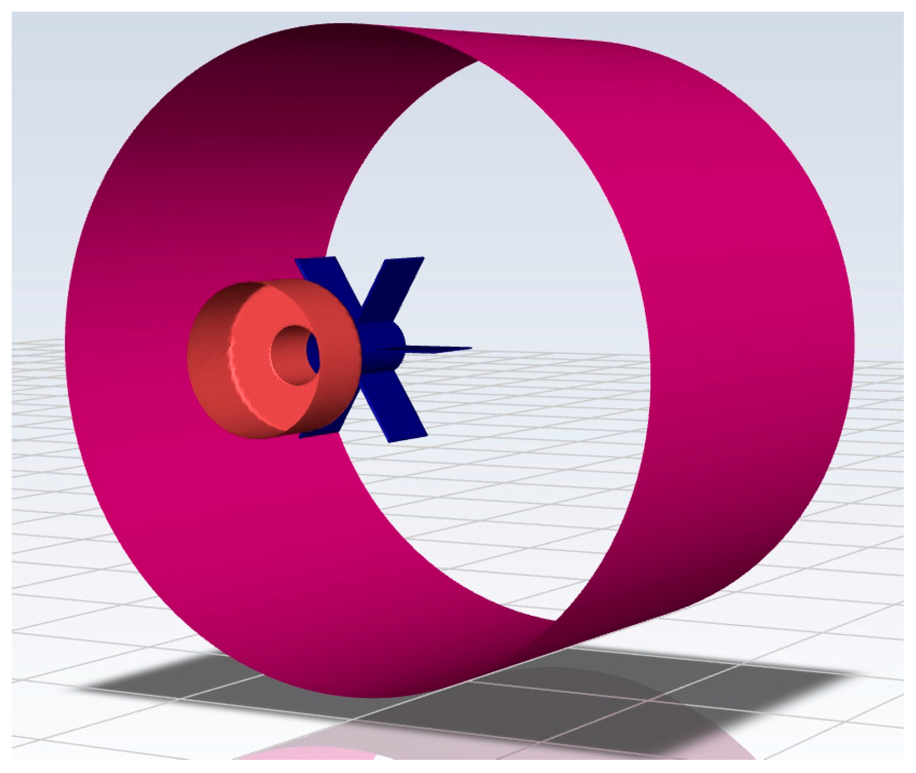
2.4.1. Establishment of the Simulation Model of GÖTEBORG 1

In this study, the GÖTEBORG 1 culture chamber model, as described in the literature [10], was used as the basis for numerical simulation. The model was reconstructed and analyzed using Ansys Fluent to verify the accuracy of the computational method proposed in this paper. A scaling ratio of 1:5 was adopted. Since the original literature did not provide complete geometric data, the key structural dimensions were measured and reconstructed based on proportional estimation methods. As the experiment focuses solely on the overlying water body, the simulation was correspondingly limited to modeling only this region. The main geometric parameters of the model are presented in

Table 1. Main data of the benthic chamber in GÖTEBORG 1.

Parameters	Actual Size	Model
size (λ)	1	1:5
height (mm)	1000	200
diameter (mm)	750	150
shaft length (mm)	270	54
shaft axis	eccentric	eccentric
blade	evenly distributed six blades	evenly distributed six blades

and Figure 1.

As this study focuses solely on the hydrodynamic characteristics of the overlying water in the culture chamber, the simulation model includes only the overlying water above the sediment layer, which accounts for approximately 50% of the chamber volume, as shown in Figure 1. After establishing the model, preliminary flow field data were obtained [28,29,30], and a tracer model was subsequently introduced, as illustrated in Figure 2. In the figure, the blue region represents the water body, while the red region represents the tracer. The physical properties of both the tracer and the water are listed in

Table 2. Computational parameters for water and tracer.

	Density (kg/m3)	$\mathbf{Viscosity}(\mathbf{k}\mathbf{g}·{\mathbf{m}}^{-1}·{\mathbf{s}}^{-1}$)	Model Height (mm)
water	998.2	0.001003	450
tracer	998.2	0.001003	50

. Since the tracer is diluted by a factor of 1000 prior to use, its physical parameters are approximately equivalent to those of the water.

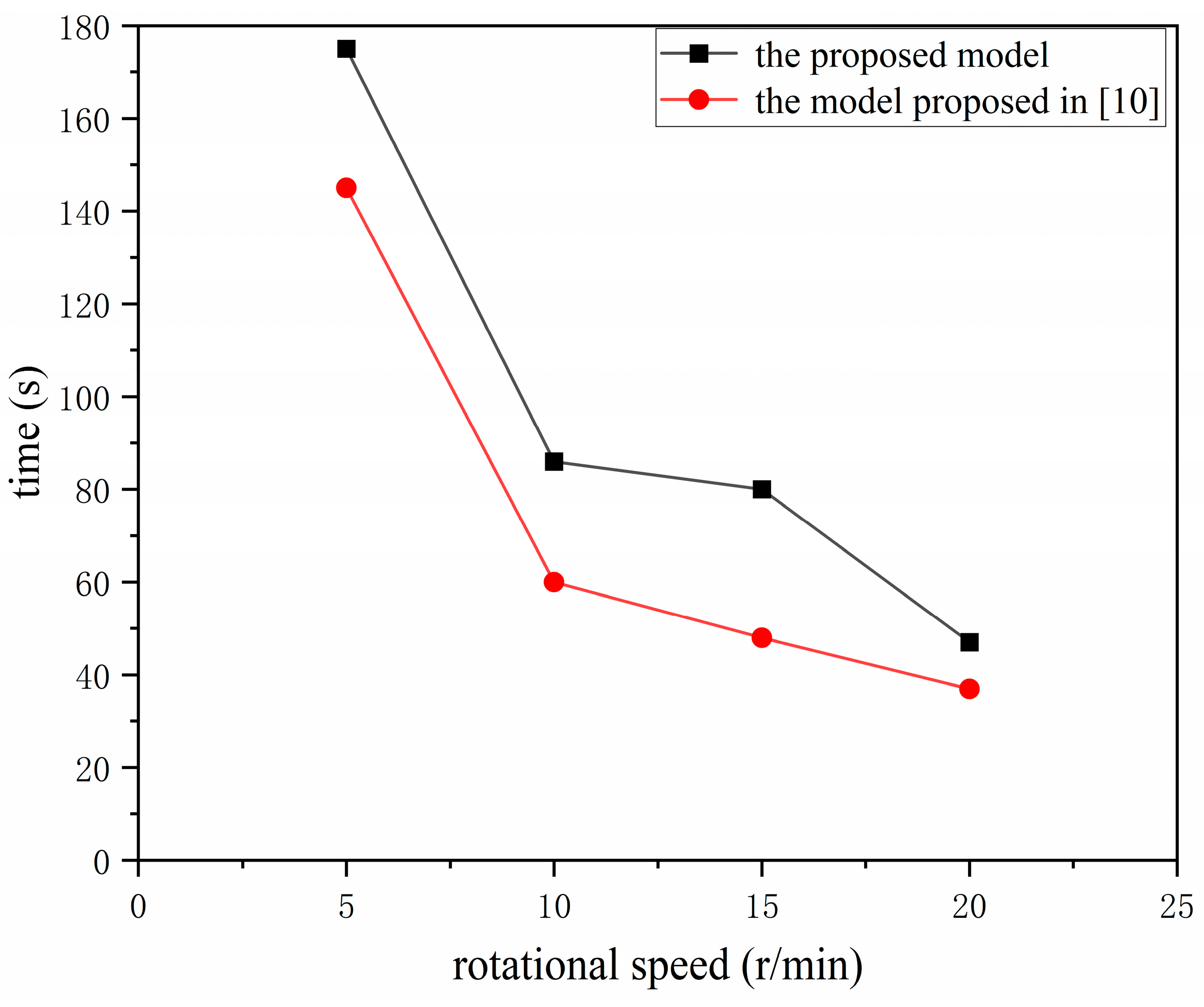
2.4.2. Simulation Verification of Calibration Method

Eight monitoring points were evenly distributed from top to bottom along the inner wall of the chamber to record changes in tracer concentration at each location. These data were used to evaluate the overall mixing efficiency within the chamber.

The mixing process was analyzed based on the following mixing equation:

$$C_3={\displaystyle \frac{C_1{V}_1+C_2{V}_2}{V_1+V_2}}$$

(12)

where C₁ is the concentration of the first solution; V₁ is the volume of the first solution; C₂ is the concentration of the second solution; V₂ is the volume of the second solution; and C₃ is the concentration of the mixed solution.

The uniformly mixed time calculated by the model in this study corresponds to the experimental mixing time reported in reference [10], as shown in Figure 3. In the speed range of 5 to 10 rpm, the slope of the mixing time curve in this study closely matches that of the literature model, indicating a high degree of consistency. However, when the stirring speed increases to between 10 and 15 rpm, a noticeable decrease in the slope is observed. This trend suggests a transitional regime between laminar and turbulent flow occurring around 10 rpm, which is consistent with conclusions reported in previous studies.

Despite the general agreement in trend, a significant discrepancy is observed in the absolute values of the mixing time required for full homogenization. This deviation is likely attributed to limitations in reconstructing the exact geometric dimensions of the reference model, particularly the blade geometry, as well as possible mismatches between the assumed boundary conditions in the simulation and the actual experimental conditions. As the rotation speed further increases beyond 20 rpm, the mixing process becomes increasingly dominated by high-intensity turbulence. In this regime, the effect of velocity gradients is enhanced, while the influence of structural details of the device becomes relatively less significant. Consequently, the differences between the simulation results of this study and the literature data become smaller at higher stirring speeds.

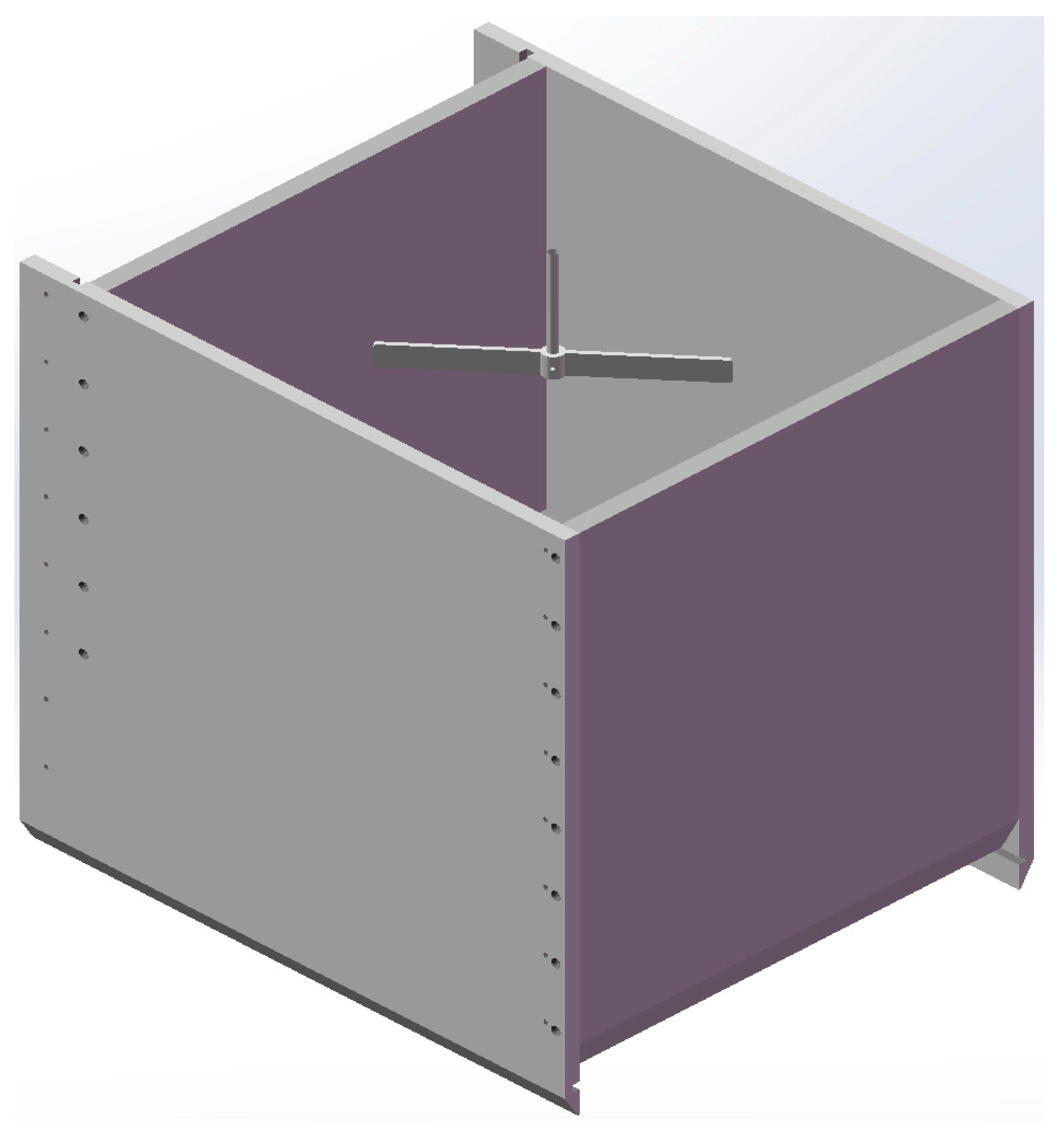
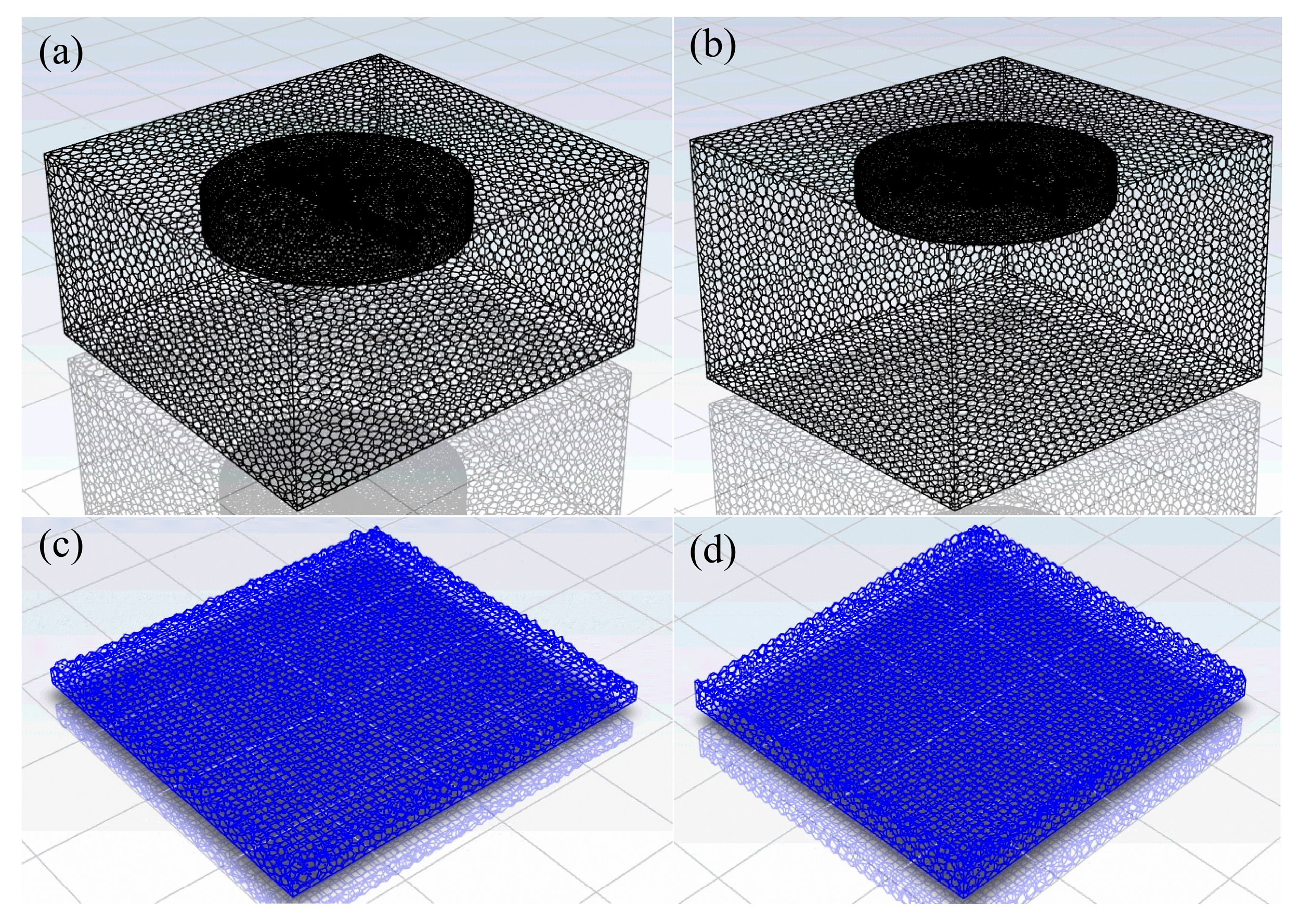
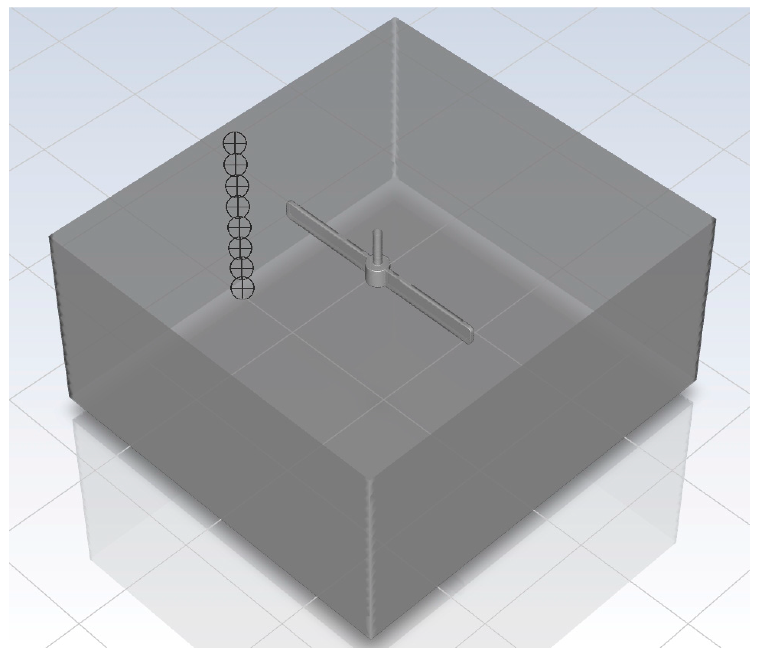
2.5. Simulation Model Establishment

According to the research in the literature [10], the influence of different culture chamber designs on the flux measurement results is limited. Therefore, for this marine in situ culture device, a square chamber design was selected to facilitate a more convenient sampling mechanism. Regarding the stirring blade structure, compared to a single-blade configuration, impellers with two or three blades have been shown to achieve a better mixing performance by enhancing the particle temperature distribution and diffusion rates [31,32,33,34]. Additionally, vertical stirrers generate lower static pressure during operation compared to horizontal ones [10]. Based on these considerations, a vertical double-blade stirring paddle design was adopted in this study, as illustrated in Figure 4.

In terms of simulation model design, this study adopts the same modeling approach as the GÖTEBORG 1 model, with specific calculations focused on the overlying water region. Based on over 90 sediment sampling datasets collected by the research team using marine landers, the insertion depth of the culture chamber into the sediment typically ranges from 20 cm to 25 cm. Accordingly, simulation analyses were conducted under two representative working conditions corresponding to sediment depths of 20 cm and 25 cm.

The model setup involves dividing the region containing the stirrer into a rotating (dynamic) domain, while the remaining area is designated as a static domain. A dynamic–static interface is defined between them. The entire computational domain is then meshed using the poly-hexcore grid method, which provides better conformity to complex boundary geometries, as illustrated in Figure 5.

Specifically, the rotational region around the stirring paddle is defined as the dynamic domain, and all other regions in the chamber are assigned as the static domain. Detailed parameters of the computational domain settings are provided in

Table 3. Details of each computational domain.

	Length	Width	Height	Circumference
205 mm sediment calculation domain	323	300	205
155 mm sediment calculation domain	323	300	155
stirring paddle rotation domain (mm)	30	0		1276

. To enhance the computational accuracy, the mesh size is configured according to the mechanical model characteristics: the minimum structural unit thickness for the stirring blade is 3 mm, hence the global mesh size is set between 1.5 mm and 10 mm.

Given the complexity of flow phenomena in the rotating region, local mesh refinement is applied around the stirring paddle and its adjacent flow field, with a minimum grid size of 1.5 mm and a maximum of 4 mm, as shown in Figure 5.

Upon completion of meshing, a quality check is conducted. Surface mesh skewness is confirmed to be well below the threshold value of 0.85, indicating high surface quality. A volume mesh comprising 134,009 cells is then generated. After mesh optimization, only 0.1% of the cells exhibit a minimum orthogonal quality below 0.5, demonstrating that the overall mesh quality is high and suitable for accurate CFD simulation.

2.6. Cabin Parameter Calculation and Calibration

The rotational coordinates in the computational model are set at the origin (0,0,0), with the rotation axis aligned along the y-direction (set to 1), while the other directions are set to 0. For each working condition at the two sediment depths, the rotation speed of the dynamic domain is varied using a stepwise gradient test method with increments of 5 rpm. The static domain shares the same rotation axis direction as the dynamic domain; however, since it borders the dynamic domain, its rotation speed is fixed at 0 rpm. The Fluent simulation parameters are detailed in

Table 4. Key computational parameter settings for the fluent model.

Setting Name	Specific Option or Value
turbulence model	RNG K-epsilon
multi-phase flow model	VOF
energy model	Off
computational model	MRF
meshing method	poly-hexcore
species model	species transport
surface tension coefficient	0.073 N/m
time step	0.01 s
rotational speed of the model with an overlying water height of 155 mm	5~60 r/min
rotational speed of the model with an overlying water height of 205 mm	0~70 r/min

. After completing the steady-state calculations, the tracer model is introduced, as illustrated in Figure 5b,d.

In previous parameter calibration studies, calibration within the chamber has primarily focused on the DBL, mixing time, and resuspension at different impeller speeds. However, according to the findings of reference [10], although the DBL thickness may vary under different experimental conditions, it generally has a negligible effect on the measured solute flux. Therefore, this paper concentrates on achieving rapid and complete mixing of the overlying water without causing resuspension. For the model with an overlying water height of 155 mm, eight monitoring points are evenly distributed vertically along the XY plane near the chamber wall, as shown in Figure 6. The time required for each point to reach full mixing at various stirring speeds is presented in Figure 7. For the model with a 205 mm water height, the calibration procedure is identical to that of the 155 mm model, with the only difference being the increased height by 50 mm.

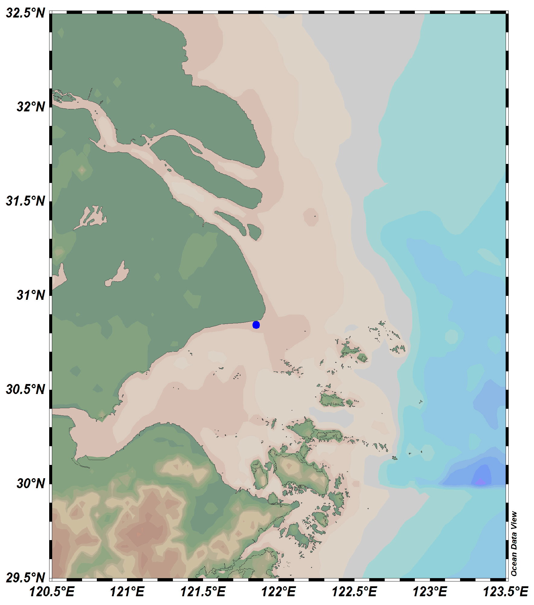
3. Experimental Environment

3.1. Experimental Preparation

To simulate submarine environments for laboratory-based in situ cultivation experiments, it is essential to maintain the physical characteristics of the overlying water and sediment substrates comparable to those of natural marine settings, even though the physicochemical properties of experimental materials may differ from actual seabed conditions. In this study, seawater and clayey sediments were collected from the muddy tidal flat of Shanghai Nanhui (coordinates: 30°50′55.8″ N, 121°50′47.6″ E; see Figure 8 and Figure 9). An acrylic tank measuring 45 × 55 × 75 cm was used as the experimental container, providing sufficient space to fully immerse the in situ cultivation devices. The tank was filled with an adequate amount of sediment and seawater, after which the in situ cultivation system was installed with ventilation valves kept open. The entire system was stabilized for one week prior to conducting subsequent experiments.

3.2. Mixing Time and Stirred Flow Field Experiment

The experimental schematic is shown in Figure 10b. Under sediment depth conditions of 20 cm (corresponding to an overlying water height of 155 mm), a gradient testing method was applied, starting at 5 rpm with increments of 5 rpm. A rubber mat, matching the chamber’s cross-sectional area, was placed horizontally above the sediment to prevent resuspension caused by high stirring speeds, which could affect the observation of mixing time. Then, a diluted fluorescent tracer was injected, and the color changes were visually monitored. The complete mixing time from the bottom to the overlying water and flow field changes were estimated using computer-synchronized timers and visual observation. The experimental setup is illustrated in Figure 10a.

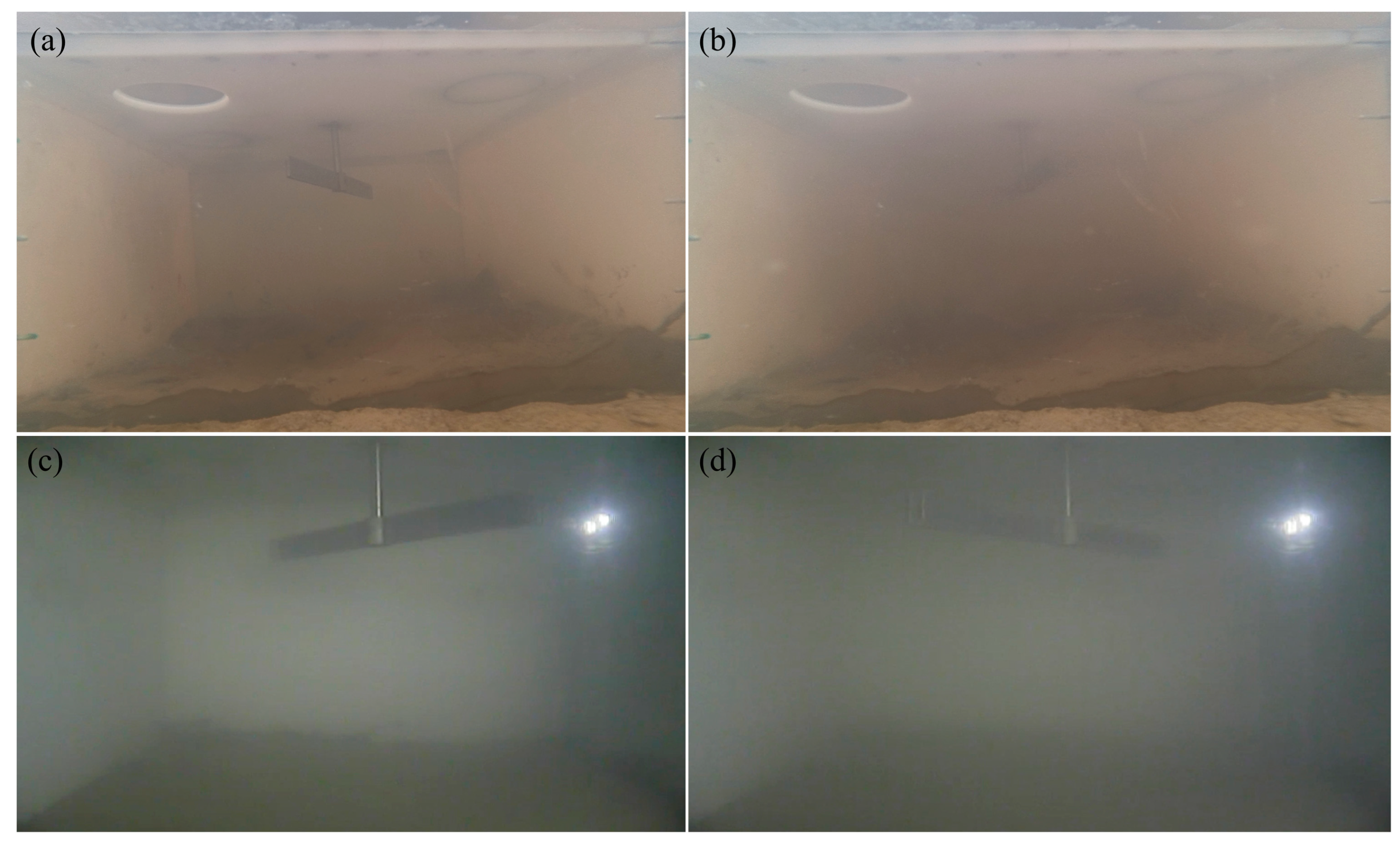
3.3. Dissolved Oxygen and Resuspension Experiment

After the aforementioned experiments, the rubber mat was removed, and the system was allowed to stabilize for at least 12 h to ensure consistent turbidity inside and outside the cultivation chamber, thereby stabilizing the concentration field at the sediment–water interface. Using the same gradient testing protocol (starting at 5 rpm with 5 rpm increments), resuspension patterns within the chamber were monitored through an aquatic imaging system combined with laboratory visual inspection. Dissolved oxygen sensors were installed both inside and outside the chamber to record oxygen concentration changes, enabling the construction of a time-resolved dissolved oxygen flux curve. The experimental setup is depicted in Figure 10c.

4. Discussion of the Results from Numerical Simulation and Model Testing

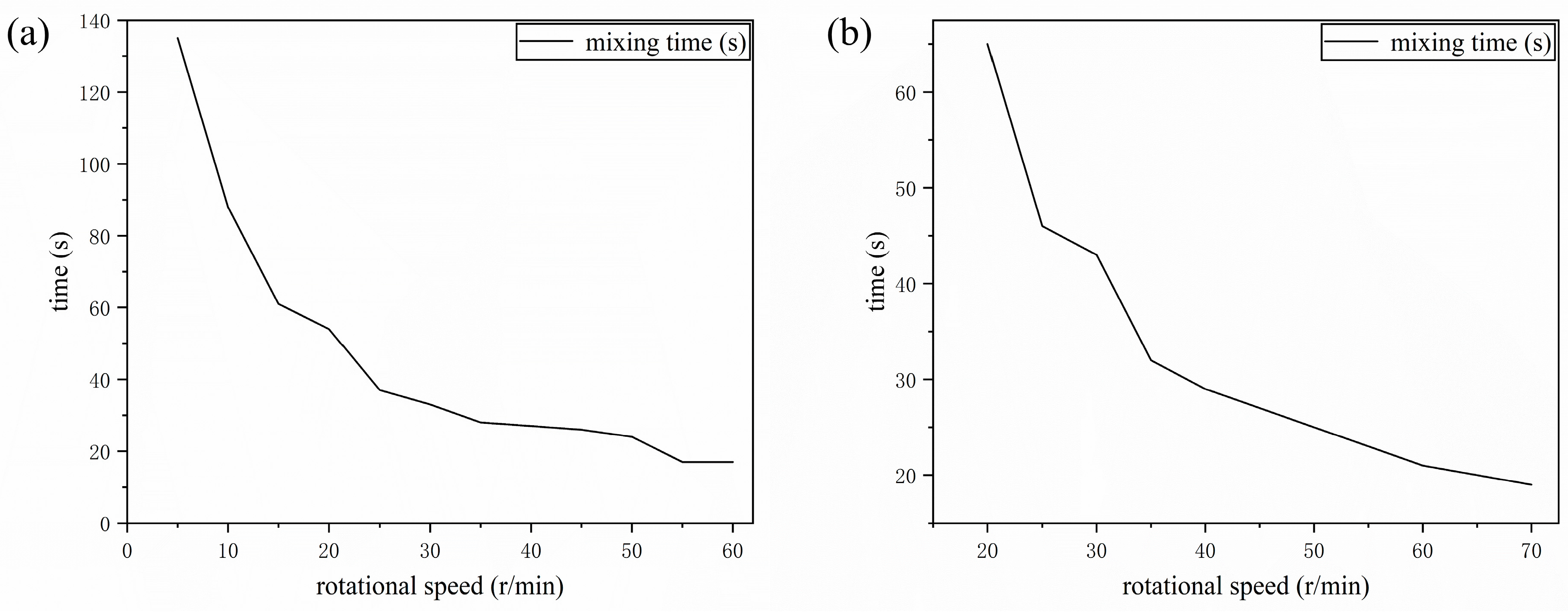
4.1. Comparison of the Complete Mixing Time

Based on the simulation results and prior experience, the actual experiments in this study focused only on cases where the complete mixing time exhibited significant variation with changes in impeller speed, thereby improving time efficiency and conserving materials. The comparison between simulation and experimental results is summarized in

Table 5. Comparison of simulation results and actual results at different rotation speeds.

Sediment Depth (mm)	Stirrer Speed (r/min)	Experimental Full Mixing Time (s)	Simulation Full Mixing Time (s)
155	20	60–64	65
155	25	42–46	46
155	30	40–44	43
155	35	33–34	32
155	40	28–30	29
155	45	25–27	27
155	50	-	25
155	55	-	23
155	60	-	21
155	65	-	20
155	70	-	19
205	5	-	135
205	10	-	88
205	15	63–67	61
205	20	50–54	54
205	25	37–39	37
205	30	31–33	33
205	35	27–29	28
205	40	28–30	27
205	45	-	26
205	50	-	24
205	55	-	17
205	60	-	17

. For the 20 cm sediment chamber model, a sharp decrease in mixing time is observed near 25 rpm, marking the transition zone from laminar to turbulent flow, as shown in Figure 7a. The deviation between simulated and measured mixing times falls within −9.23% to 9.25%. Similarly, in the 15 cm sediment chamber model, a pronounced change in the mixing time gradient occurs beyond 35 rpm, as shown in Figure 7b, with deviations ranging from −9.4% to 9.1%.

Overall, the difference between simulated and experimental complete mixing times is limited to just a few seconds, indicating strong agreement between the two approaches.

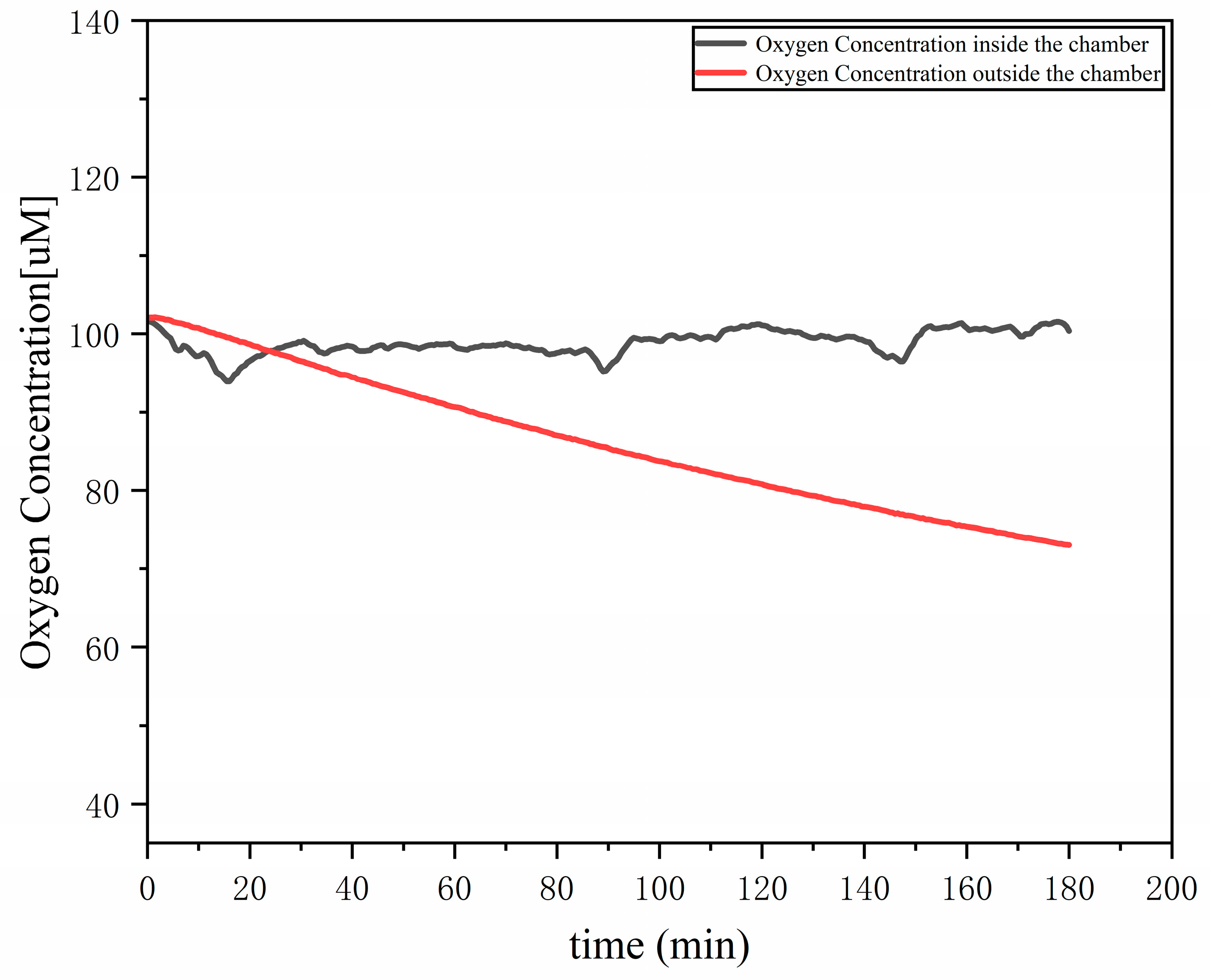
4.2. Oxidation Consumption and Resuspension

From Experiments in Section 3.3, it was observed that the rotational speeds triggering sediment resuspension were approximately 40 r/min and 35 r/min for sediment depths of 15 cm and 20 cm, respectively, as shown in Figure 11. Figure 12 illustrates the dissolved oxygen trends inside and outside the cultivation chamber. The dissolved oxygen outside the chamber remained relatively stable, whereas a steady decline was observed inside the chamber, indicating that the in situ cultivation process was proceeding normally.

It is important to note that the experiment was not conducted under deep-sea conditions, and the properties of the experimental materials (e.g., sediment and seawater) continuously changed over time. Additionally, manual replacement of seawater inside and outside the chamber was required after each test. Therefore, the dissolved oxygen data presented here should be interpreted primarily as indicative of the declining trend, rather than as absolute quantitative values.

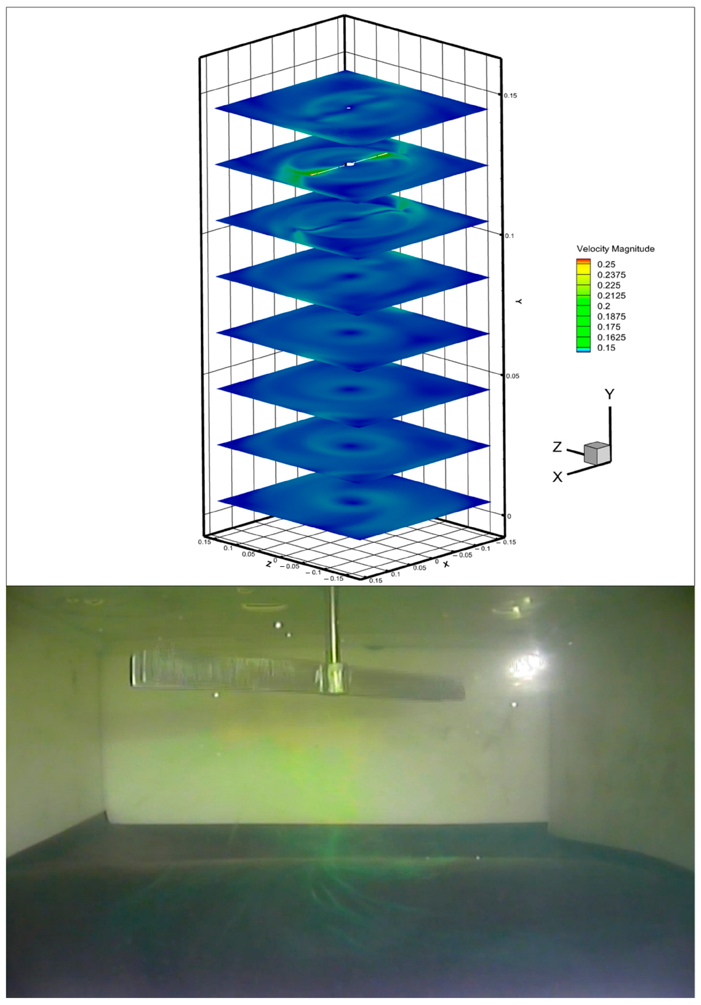
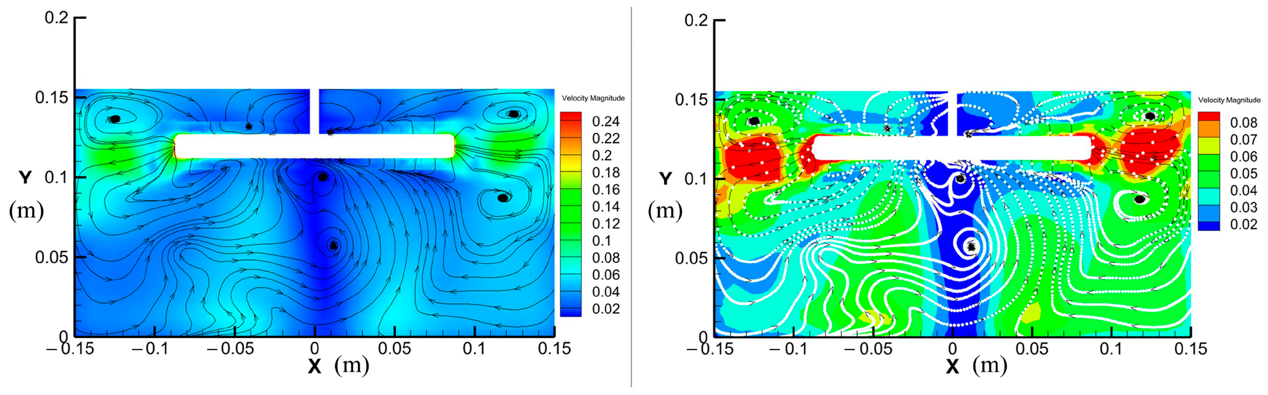
4.3. Analysis of Flow Field Characteristics Inside the Cultivation Chamber

Figure 13 shows the flow field characteristics inside the cultivation chamber simulated using Tecplot 360 EX 2024 R1 software. It illustrates the velocity distribution at eight monitoring points across the cross-section and XY plane, clearly reflecting both the magnitude and direction of fluid flow. The color gradient intuitively represents the flow speed distribution. By comparing the simulation results with experimental observations at calibrated rotational speeds, a strong spatial consistency between the two is evident:

(1) Flow Field Symmetry: In terms of flow field symmetry, the predicted axis of the dual vortex structure (the plane where the stirring blades are located) in the numerical simulation aligns with the tracer particle motion trajectories in the actual experiment, validating the radial dominant characteristic of the central dual-blade stirring.

(2) Velocity Distribution: In the simulation, the high-velocity region (0.2–0.25 m/s) near the paddle—marked in green—corresponds to the tracer particle aggregation zones in the experimental images. A low-velocity zone is also observed beneath the stirrer, likely due to the formation of a primary vortex. Shear forces and centrifugal effects generated by paddle rotation significantly reduce fluid velocity in this area.

(3) Flow Field Consistency: The velocity distributions across all eight sections demonstrate a high degree of uniformity, suggesting that the stirrer design effectively promotes a consistent flow field. This uniformity improves both mixing efficiency and the accuracy of flux measurements at the sediment–water interface.

Further analysis reveals that tracer particles follow the streamlines of the flow. Particles near the paddle tips exhibit higher velocities, while those approaching chamber walls experience a “wall-avoidance effect.” The vortex structures formed at the blade trailing edge reveal the existence of a Kármán vortex street, a phenomenon commonly observed in flows past bluff bodies and characterized by a regular pattern of alternating vortex shedding on either side. This phenomenon contributes to increased local turbulence and enhanced mixing. Owing to the stirrer’s constant rotational speed, the vortices within the chamber demonstrate stable behavior, culminating in a steady-state flow field and particle distribution, as illustrated in Figure 14.

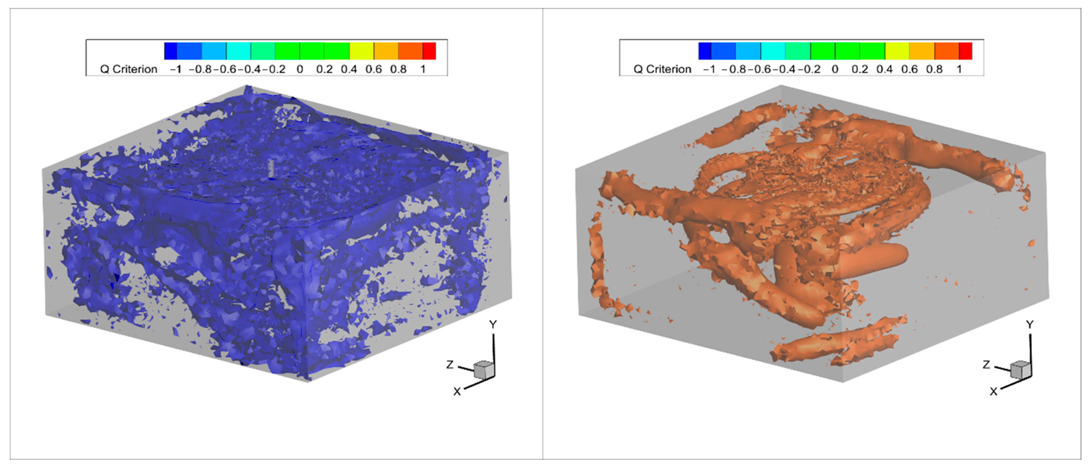
4.4. Evolution of Vortex Structure and Flow Field Stability During the Stirring Process

The distribution of vorticity within the flow field offers a more intuitive depiction of dynamic fluid behavior. As shown in Figure 15, the CFD simulation results reveal that during the initial stage of stirring, the flow field exhibits numerous vortex structures and intense fluid motion. Small-scale vortices dominate the flow at this stage, resulting in high vorticity due to strong viscous dissipation. As stirring continues, these small vortices gradually dissipate as a result of viscosity, leading to a reduction in fluid kinetic energy and a decline in flow irregularity. Consequently, the flow field begins to stabilize. During this stabilization phase, while some vortices vanish, new vortex structures may also emerge; however, the overall number of vortices decreases over time [35].

This evolution reflects the inherently dynamic nature of fluid motion within the cultivation chamber—characterized by continuous reorganization of vortex structures. As the flow field becomes more stable, the decreasing number of vortices promotes a more uniform fluid flow, contributing to a consistent velocity distribution, a more stable DBL thickness, and more uniform shear stress within the chamber.

5. Conclusions

The rational calibration of stirring speed is a critical factor in balancing effective mixing with the risk of sediment resuspension. This study precisely identifies the flow field transition zones and resuspension thresholds for two sediment depths by integrating CFD simulations with laboratory experiments. These findings provide a scientific basis for calibrating operational parameters of in situ cultivation devices. When the stirring speed is too low, mixing efficiency in the overlying water is inadequate, leading to incomplete mixing and reducing the reliability of solute flux measurements. Conversely, excessive stirring speeds cause sediment resuspension, disrupt the authenticity of the in situ environment, and increase flux measurement errors. The proposed method offers a new strategy for chamber parameter calibration and the design of in situ cultivation systems, enhancing the quality and reliability of observational data. Simulation results show that at calibrated stirring speeds, the dual-vortex structure generated by the impeller maintains flow field symmetry. As the flow field stabilizes, vortex dissipation reaches equilibrium, ensuring a uniform physical environment for accurate elemental flux measurements.

The calibration method and device design proposed in this study enable the tuning of stirring parameters for various types of in situ cultivation systems by simply adjusting the model’s boundary conditions. Compared to traditional approaches, this method allows for the precise calibration of parameters that achieve both complete fluid mixing and the prevention of sediment resuspension. For the device examined in this study, a stirring speed of 25 r/min is optimal when the sediment depth is 20 cm, ensuring full mixing without triggering resuspension. Likewise, at a sediment depth of 15 cm, the optimal stirring speed is 35 r/min. At these calibrated critical conditions, flow field uniformity, mixing efficiency, and resuspension suppression are simultaneously optimized. In conclusion, this study provides scientific guidance for the design and operation of future in situ cultivation devices and proposes a novel parameter calibration method. Further deep-sea experiments will be conducted to verify the applicability of this method in deep-sea in situ observations, where environmental stability and measurement accuracy are critically important.

References

1. Donis, D.; McGinnis, D.F.; Holtappels, M.; Felden, J.; Wenzhoefer, F. Assessing benthic oxygen fluxes in oligotrophic deep sea sediments (HAUSGARTEN observatory). Deep Sea Res. Part I Oceanogr. Res. Pap. 2016, 111, 1–10. [Google Scholar] [CrossRef]
2. Lee, J.S.; Kim, S.-H.; Min, W.-G.; Choi, D.M.; Lee, E.K.; Kim, K.-T.; An, S.-U.; Baek, J.-W.; Lee, W.-C.; Park, C.H. In-Situ Estimates of Net Ecosystem Metabolisms in the Rocky Habitats of Dokdo Islets in the East Sea of Korea. J. Mar. Sci. Eng. 2022, 10, 887. [Google Scholar] [CrossRef]
3. Ruan, D.; Chen, J.; Wang, H.; Peng, X.; Zhou, P.; He, W. Development of a Hadal Microbial In Situ Multi-Stage Filtering and Preserving Device. J. Mar. Sci. Eng. 2021, 9, 1424. [Google Scholar] [CrossRef]
4. Wang, Y.; Gao, Z.-M.; Li, J.; He, L.-S.; Cui, G.-J.; Li, W.-L.; Chen, J.; Xin, Y.-Z.; Cai, D.-S.; Zhang, A.-Q. Hadal water sampling by in situ microbial filtration and fixation (ISMIFF) apparatus. Deep Sea Res. Part I Oceanogr. Res. Pap. 2019, 144, 132–137. [Google Scholar] [CrossRef]
5. Garel, M.; Bonin, P.; Martini, S.; Guasco, S.; Roumagnac, M.; Bhairy, N.; Armougom, F.; Tamburini, C. Pressure-retaining sampler and high-pressure systems to study deep-sea microbes under in situ conditions. Front. Microbiol. 2019, 10, 453. [Google Scholar] [CrossRef]
6. Kononets, M.; Tengberg, A.; Nilsson, M.; Ekeroth, N.; Hylén, A.; Robertson, E.K.; Van De Velde, S.; Bonaglia, S.; Rütting, T.; Blomqvist, S. In situ incubations with the Gothenburg benthic chamber landers: Applications and quality control. J. Mar. Syst. 2021, 214, 103475. [Google Scholar] [CrossRef]
7. Broman, E.; Olsson, M.; Maciute, A.; Donald, D.; Humborg, C.; Norkko, A.; Jilbert, T.; Bonaglia, S.; Nascimento, F.J. Biotic interactions between benthic infauna and aerobic methanotrophs mediate methane fluxes from coastal sediments. ISME J. 2024, 18, wrae013. [Google Scholar] [CrossRef]
8. Zhao, G.T.; Yu, X.S.; Li, X.; Shun, J.; Zhang, X.D.; Zhang, S.W.; Wang, X.N.; Li, F.Z.; Cao, R.X.; Xu, C.L. Benvir: A in situ Deep-sea observation system for Benthic environmental monitoring. High Technol. Lett. 2015, 25, 54–60. [Google Scholar]
9. Xu, C.C. Benthic Flux Chamber of Self-Adaptive Stirring. Master’s Thesis, Zhejiang University, Hangzhou, China, 2017. [Google Scholar]
10. Tengberg, A.; Hall, P.O.; Andersson, U.; Lindén, B.; Styrenius, O.; Boland, G.; De Bovee, F.; Carlsson, B.; Ceradini, S.; Devol, A. Intercalibration of benthic flux chambers: II. Hydrodynamic characterization and flux comparisons of 14 different designs. Mar. Chem. 2005, 94, 147–173. [Google Scholar] [CrossRef]
11. Khedr, A.; Castellani, F. Critical issues in the moving reference frame CFD simulation of small horizontal axis wind turbines. Energy Convers. Manag. X 2024, 22, 100551. [Google Scholar] [CrossRef]
12. Rave, K.; Hermes, M.; Wirz, D.; Hundshagen, M.; Friebel, A.; von Harbou, E.; Bart, H.-J.; Skoda, R. Experiments and fully transient coupled CFD-PBM 3D flow simulations of disperse liquid-liquid flow in a baffled stirred tank. Chem. Eng. Sci. 2022, 253, 117518. [Google Scholar] [CrossRef]
13. Haddadi, M.; Hosseini, S.; Rashtchian, D.; Olazar, M. Comparative analysis of different static mixers performance by CFD technique: An innovative mixer. Chin. J. Chem. Eng. 2020, 28, 672–684. [Google Scholar] [CrossRef]
14. Wen, M.; Shan, H.; Zhang, S.; Guo, L.; Liu, X.; Jia, Y. Resuspension of sediments along the bottom boundary layer: A review. Mar. Geol. Quat. Geol. 2016, 36, 177–188. [Google Scholar]
15. De La Concha-Gómez, A.; Ramírez-Muñoz, J.; Márquez-Baños, V.; Haro, C.; Alonso-Gómez, A. Effect of the rotating reference frame size for simulating a mixing straight-blade impeller in a baffled stirred tank. Rev. Mex. De Ing. Química 2019, 18, 1143–1160. [Google Scholar] [CrossRef]
16. Bakker, A.; LaRoche, R.D.; Wang, M.-H.; Calabrese, R.V. Sliding mesh simulation of laminar flow in stirred reactors. Chem. Eng. Res. Des. 1997, 75, 42–44. [Google Scholar] [CrossRef]
17. Reid, A.; Rossi, R.; Cottini, C.; Benassi, A. CFD simulation of a Rushton turbine stirred-tank using open-source software with critical evaluation of MRF-based rotation modeling. Meccanica 2024, 1–25. [Google Scholar] [CrossRef]
18. Coroneo, M.; Montante, G.; Paglianti, A.; Magelli, F. CFD prediction of fluid flow and mixing in stirred tanks: Numerical issues about the RANS simulations. Comput. Chem. Eng. 2011, 35, 1959–1968. [Google Scholar] [CrossRef]
19. Duan, X.; Feng, X.; Mao, Z.-S.; Yang, C. Numerical simulation of reactive mixing process in a stirred reactor with the DQMOM-IEM model. Chem. Eng. J. 2019, 360, 1177–1187. [Google Scholar] [CrossRef]
20. Mouketou, F.N.; Kolesnikov, A. Modelling and simulation of multiphase flow applicable to processes in oil and gas industry. Chem. Prod. Process Model. 2019, 14, 20170066. [Google Scholar] [CrossRef]
21. Pozzetti, G.; Peters, B. A multiscale DEM-VOF method for the simulation of three-phase flows. Int. J. Multiph. Flow 2018, 99, 186–204. [Google Scholar] [CrossRef]
22. Li, W.; Wu, W.; Miao, Q.; Wu, J. Research on the Overall Design and Water Entry Simulation of Cross-Media Unmanned Underwater Vehicles. J. Mar. Sci. Eng. 2025, 13, 78. [Google Scholar] [CrossRef]
23. Ye, Z.; Zhao, X. Investigation of water-water interface in dam break flow with a wet bed. J. Hydrol. 2017, 548, 104–120. [Google Scholar] [CrossRef]
24. Ghaini, A.; Mescher, A.; Agar, D.W. Hydrodynamic studies of liquid–liquid slug flows in circular microchannels. Chem. Eng. Sci. 2011, 66, 1168–1178. [Google Scholar] [CrossRef]
25. Hao, L.; Liu, Z.; Hu, C.Y. Comparison of differences in simulating nearshore currents with different turbulence models. China Harb. Eng. 2022, 42, 1–6. [Google Scholar]
26. Speziale, C.G.; Thangam, S. Analysis of an RNG based turbulence model for separated flows. Int. J. Eng. Sci. 1992, 30, 1379–1388. [Google Scholar] [CrossRef]
27. Ahn, S.-H.; Xiao, Y.; Wang, Z.; Luo, Y.; Fan, H. Unsteady prediction of cavitating flow around a three dimensional hydrofoil by using a modified RNG k-ε model. Ocean Eng. 2018, 158, 275–285. [Google Scholar] [CrossRef]
28. Luo, J. Full flow field computation of mixing in baffled stirred vessels. Trans. Inst. Chem. Eng. 1993, 71, 342–344. [Google Scholar]
29. Yapici, K.; Karasozen, B.; Schäfer, M.; Uludag, Y. Numerical investigation of the effect of the Rushton type turbine design factors on agitated tank flow characteristics. Chem. Eng. Process. Process Intensif. 2008, 47, 1340–1349. [Google Scholar] [CrossRef]
30. Siddiqui, M.S.; Khalid, M.H.; Badar, A.W.; Saeed, M.; Asim, T. Parametric analysis using cfd to study the impact of geometric and numerical modeling on the performance of a small scale horizontal axis wind turbine. Energies 2022, 15, 505. [Google Scholar] [CrossRef]
31. Ebrahimi, M.; Yaraghi, A.; Ein-Mozaffari, F.; Lohi, A. The effect of impeller configurations on particle mixing in an agitated paddle mixer. Powder Technol. 2018, 332, 158–170. [Google Scholar] [CrossRef]
32. Biggs, R. Mixing rates in stirred tanks. AIChE J. 1963, 9, 636–640. [Google Scholar] [CrossRef]
33. Jongen, T. Characterization of batch mixers using numerical flow simulations. AIChE J. 2000, 46, 2140–2150. [Google Scholar] [CrossRef]
34. Wu, M.; Wu, C.; Liang, J.; Lei, Y.; Yang, B. Study on shear properties of six kinds of conventional agitator. Huaxue Gongcheng/Chem. Eng. China 2017, 45, 68–73. [Google Scholar]
35. Siddiqui, M.S.; Fonn, E.; Kvamsdal, T.; Rasheed, A. Finite-volume high-fidelity simulation combined with finite-element-based reduced-order modeling of incompressible flow problems. Energies 2019, 12, 1271. [Google Scholar] [CrossRef]
Figure 1. The model of GÖTEBORG 1 chamber.
Jmse 13 01290 g001
Figure 2. Schematic contour map of tracer distribution inside the chamber.
Jmse 13 01290 g002
Figure 3. Comparison of the mixing time calculated by the model in this study with that of GÖTEBORG 1 (reference [10]).
Jmse 13 01290 g003
Figure 4. Benthic chamber and stirring paddle design.
Jmse 13 01290 g004
Figure 5. Grid conditions in the chamber: (a) Grid of overlying water at a sediment height of 20 cm; (b) corresponding tracer grid; (c) grid of overlying water at a sediment height of 15 cm; (d) corresponding tracer grid.
Jmse 13 01290 g005
Figure 6. Locations of monitoring points inside the chamber.
Jmse 13 01290 g006
Figure 7. (a) Relationship between rotational speed and time to complete mixing for a sediment height of 205 mm; (b) Relationship between rotational speed and time to complete mixing for a sediment height of 155 mm.
Jmse 13 01290 g007
Figure 8. Sampling points.
Jmse 13 01290 g008
Figure 9. On-site sampling photograph.
Jmse 13 01290 g009
Figure 10. (a) Experimental setup for observing complete mixing time; (b) schematic diagram of the overall apparatus; (c) experimental setup for dissolved oxygen and resuspension test.
Jmse 13 01290 g010
Figure 11. When the sediment depth is 20 cm, (a) represents the pre-mixing state, and (b) represents the post-mixing resuspension state; when the sediment depth is 15 cm, (c) represents the pre-mixing state, and (d) represents the post-mixing resuspension state.
Jmse 13 01290 g011
Figure 12. Comparison of dissolved oxygen levels inside and outside the chamber.
Jmse 13 01290 g012
Figure 13. Velocity profile at eight monitoring points and corresponding observed phenomena.
Jmse 13 01290 g013
Figure 14. Flow field and particle streamline diagrams on the XY plane.
Jmse 13 01290 g014
Figure 15. Variation of vorticity inside the chamber from the start of stirring to flow field stabilization.
Jmse 13 01290 g015