On Predicting Marine Engine Measurements with Synthetic Data in Scarce Dataset

Abstract

The scarcity of high-quality maritime datasets poses a significant challenge for machine learning (ML) applications in marine engineering, particularly in scenarios where real-world data collection is limited or impractical. This study investigates the effectiveness of synthetic data generation and cross-modeling in predicting operational metrics of LNG carrier engines. A total of 38 real-world data points were collected from port and starboard engines, focusing on four target outputs: mechanical efficiency, fuel consumption, load, and effective power. CopulaGAN, a hybrid generative model combining statistical copulas and generative adversarial networks, was employed to produce synthetic datasets. These were used to train multilayer perceptron (MLP) regression models, which were optimized via grid search and validated through five-fold cross-validation. The results show that synthetic data can yield accurate models, with mean absolute percentage errors (MAPE) below 2% in most cases. The combined synthetic datasets consistently outperformed those generated from single-engine data. Cross-modeling was partially successful, as models trained on starboard data generalized well to port data but not vice versa. The engine load variable remained challenging to predict due to its narrow and low-range distribution. Overall, the study highlights synthetic data as a viable solution for enhancing the performance of ML models in data-scarce maritime applications.

1. Introduction

The application of deep learning techniques, such as neural networks or tree-based ensembles, is continually growing in maritime applications, becoming increasingly commonplace in the research and analysis of marine-focused datasets [1]. Tran et al. [2] note the need for high-quality data for maritime detections and predictions. Researchers emphasize the need for the application of various technologies, including advanced modeling techniques [3], to mitigate negative effects, highlighting the indispensability of ML techniques in modern maritime operations [1]. Because this can be challenging due to the scarcity and low probability of certain data ranges, the authors propose the utilization of data synthetization as a possible solution. The application of this technique enables researchers to achieve high precision, even in cases where the data in real-world datasets is almost nonexistent. Majnarić et al. [4] also note the possibility of improving models for the calculation of a ship’s main particulars using synthetic data. Due to the limited number of unique ship forms, it can be hard to develop models that perform well on novel forms. Synthetic data generation allows for a wide variety of “new” ship forms to be generated, filling the dataset gaps and allowing for the improvement of prediction scores. In a similar vein, the authors of [5] demonstrate the use of synthetic data to expand a dataset consisting of steam turbine exergy measurements, allowing for a fuller dataset and providing higher-quality predictions. Feature engineering to improve scores is demonstrated by Li et al. [6] for another case of rare-event data: the problem of predicting the severity of marine accidents, where the application of advanced techniques improved the prediction score by 6.43%. Yigin and Celik [7] also applied data synthetization, namely generative adversarial networks, to fill out and expand a dataset consisting of ship machinery failures, allowing for higher precision in the created prediction models.

As the presented research demonstrates, the application of data synthetization is a growing practice in maritime applications using machine learning, especially when phenomena with naturally scarce data or rare events are considered.

Several published papers have targeted similar outputs. Nuyen et al. [8] demonstrated a fuel consumption model based on predictive machine learning models, including extreme gradient boosting machines and artificial neural networks, achieving a MAPE of 0.21%. A similar approach was applied by Hu et al. [9], achieving an $R^2$ score of 0.9817, and Melo et al. [10] achieved an $R^2$ of 0.91 under similar circumstances. Regarding energy efficiency, Karatug et al. [11] modeled it using the ANFIS method on data collected from a container vessel, achieving an error of 1.67%. Meng et al. [12] demonstrated the application of optimization algorithms using an artificial neural network for the prediction of shiploads. A similar piece of work was performed by Unlubayir et al. [13], who used the Long Short-Term Memory network and obtained a load prediction accuracy of 0.97. For the case of power prediction, many examples of such work exist, such as that by Lang et al., who applied supervised ML methods such as XGBoost, artificial neural networks, and support vector machines [14]. A similar approach was demonstrated by Zhou et al. [15] by applying a physics-informed artificial neural network to predict ship propulsion power; they achieved a MAPE of 14%.

The above papers provide a baseline as to what can be achieved when applying ML algorithms and inform the novelty of the current research article. This novelty first lies in the application of synthetic data and cross-testing between two maritime engines on the same vessel; most of the listed research either used small datasets as-is, was able to collect larger datasets, or used simulated data. The other novelty lies in the operating range of the engines. Most research focuses on the optimal, manufacturer-recommended operating range. The research in this study, the data of which will be presented in greater detail going forward, focuses on the lower end of the operating range, representing a form of analysis not present in the papers reviewed as part of this introduction.

The goal of this study is to test how ML models can be applied in situations where data is scarce and additional data collection is not possible or practical. For this reason, two approaches will be tested: cross-modeling between engines and the application of synthetic data. The study will aim to answer the following research questions (RQs):

• RQ1—Can a model based purely on synthetic data achieve satisfactory performance when evaluated on real-world data that consists of only a few data points?
• RQ2—Can cross modeling be applied, allowing researchers to model a starboard engine using the data collected from the port-side engine, or vice-versa, to lower the amount of data necessary for collection?
• RQ3—In a similar approach to cross-modeling, can a mix between the two (synthetic) data sets achieve improved scores?

The manuscript is split into four main sections. The first will describe the dataset using a narrative and statistical description of the data and how it was collected and then synthesized for further use. Then, the regression methodology itself will be described, as well as the evaluation techniques. With that section concluding the description of the used methods, the manuscript will present and discuss the results obtained. Finally, the conclusions based on the results will be given.

2. Dataset Description and Synthetization

The dataset consists of 18 measurements for each of the two engines of an LNG carrier.

The ship on which the measurements were performed is a commercial LNG (Liquefied Natural Gas) carrier. The ship has a deadweight tonnage of 104,561 tons, an overall length of 315 m, and a maximum breadth of 50 m. For the propulsion, the ship uses two identical parallel-running MAN B&W, Augsburg, Germany 6S70ME-C diesel engines (port and starboard). Each main engine directly drives its propulsion propeller – the port propeller rotates clockwise looking from aft, while the starboard propeller rotates anti-clockwise looking from aft. Along with the two identical main propulsion engines, the ship has four diesel generator engines (for electricity production) and one emergency generator engine. The main particulars of the MAN B&W 6S70ME-C diesel engine are presented in

Table 1. Main particulars of each MAN B&W 6S70ME-C diesel engine.

Particular	Value
Number of cylinders	6 inline cylinders
Stroke	2.8 m
Cylinder bore	0.7 m
Process	Two stroke
Fuel injectors per cylinder	2
Injection type	Direct injection
Fuel	Diesel-very low sulfur oil
Fuel lower heating value	42 MJ/kg
Engine speed (at Maximum Continuous Rating (MCR))	85 RPM
Power output (at MCR)	17,550 kW

.

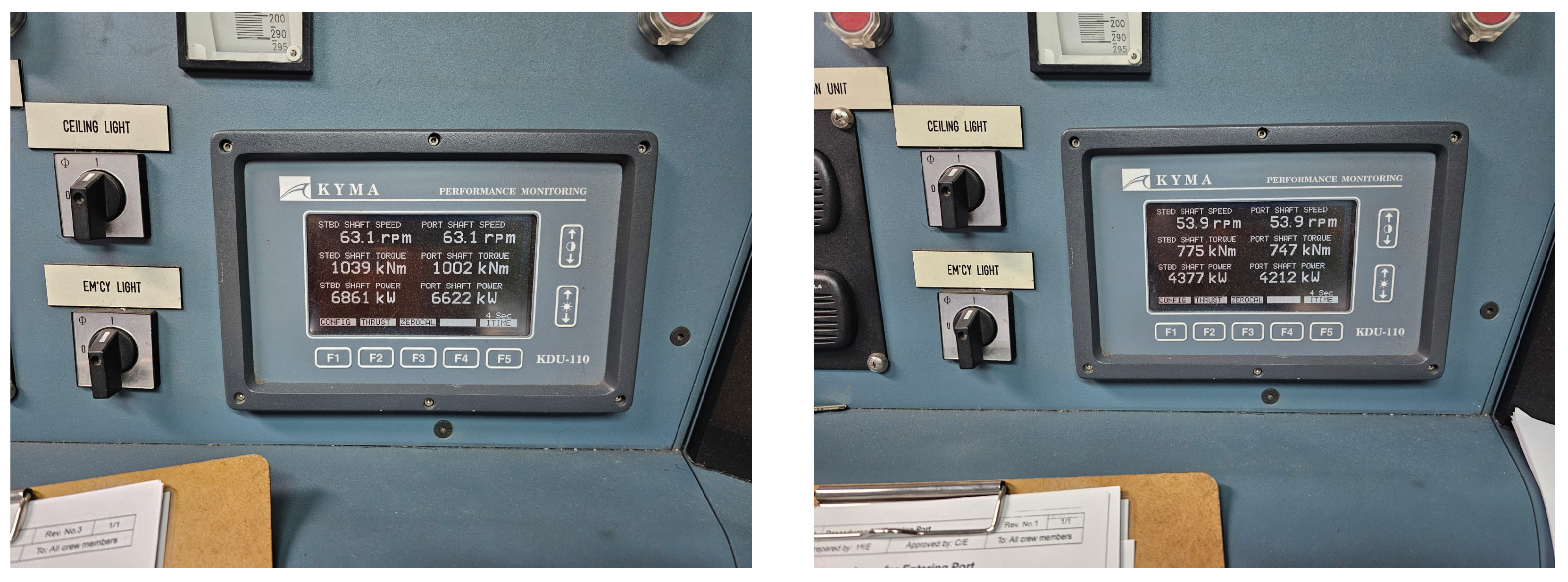
There are three measurements for each of the six cylinders in both engines at three different loads (22.95%, 36.08%, and 54.14% for the port engine and 22.28%, 35.46%, and 51.97% for the starboard engine). In addition to this, it contains information on the indicated pressure (bar) and maximum pressure in the cylinder (bar), the compression pressure in each cylinder (bar), the ratio of compression and scavenging pressure, engine speed (rpm), the effective pressure in each cylinder (bar), the indicated power (kW), the effective power (kW), mechanical losses (kW), mechanical efficiency (%), the fuel consumption of the whole engine (kg/h), the indicated efficiency of the whole engine (%), the effective efficiency of the whole engine, and the specific effective fuel consumption (g/kWh). Neither dataset contains any significant outliers or other aberrations, and no data is missing. The parameters were collected from a built-in terminal in the vessel’s operating room, as shown in Figure 1; the values not presented there (e.g., efficiency) were calculated.

Table 2. Descriptive statistics of the whole dataset, including mean, standard deviation ($\sigma$), kurtosis (Kurt.), skewness (Skew.), and minimum (Min.) and maximum (Max.) values.

Value	Mean	$\mathit{\sigma }$	Kurt.	Skew.	Min.	Max.
Indicated pressure (bar)	10.36	2.31	−1.47	0.16	7.44	14.03
Compression pressure (bar)	62.80	15.98	−1.53	0.39	48.90	90.30
Maximum pressure (bar)	94.00	14.71	−1.51	0.17	76.20	116.50
Ratio of compression and scavenging pressure	35.00	0.43	−0.75	0.29	34.30	35.90
Speed (rpm)	63.00	6.64	−1.54	−0.15	54.00	70.00
Effective pressure (bar)	9.36	2.31	−1.47	0.16	6.44	13.03
Indicated power (kW)	1172.18	383.32	−1.50	0.17	721.54	1763.80
Effective power (kW)	1059.04	371.57	−1.50	0.18	624.56	1638.08
Mechanical losses (kW)	113.14	11.93	−1.54	−0.15	96.98	125.72
Mechanical efficiency (%)	90.35	2.23	−1.45	−0.20	86.56	92.87
Fuel consumption (kg/h)	1256.98	349.80	−1.54	−0.14	783.81	1632.82
Fuel consumption engine (kg/h)	1.47	0.41	−1.54	−0.14	0.91	1.90
Indicated efficiency (%)	49.67	2.39	−1.24	0.37	47.26	53.86
Effective efficiency (%)	43.45	2.92	−1.25	0.75	42.62	49.90
Specific effective fuel consumption	194.02	11.63	−1.32	−0.71	168.92	197.81
Load	35.77	12.66	−1.52	0.17	22.28	54.14

reveals several notable aspects of engine performance and variability. The indicated pressure shows a relatively low mean of 10.36 bar with a narrow range (7.44 to 14.03 bar), suggesting stable combustion chamber conditions across cycles; its low skewness and negative kurtosis indicate a near-normal but slightly flat distribution. The compression and maximum pressures reach mean values of 62.8 bar and 94 bar, respectively, with the latter peaking at 116.5 bar. Both exhibit moderate variability, with standard deviations of around 15 and 14.7 bar. The effective and indicated power show substantial output levels, averaging 1059.03 kW and 1172.18 kW, respectively, with relatively low skewness and large standard deviations (371.6 and 383.3 kW), suggesting variations in operational loads. Mechanical losses remain consistent (a mean of 113.11 kW and a standard deviation of 11.9 kW), supporting high mechanical efficiency (mean: 90.35%; standard deviation: 2.23) and indicating reliable energy transmission. The fuel consumption rate (mean: 1256.98 kg/h) exhibits high variability (standard deviation: 349.80 kg/h), though the specific fuel consumption remains relatively stable (mean: 194.02 g/kWh), suggesting efficient scaling of fuel usage with output. The effective efficiency (mean: 43.45%) shows a more positively skewed distribution (0.748) than the indicated efficiency (mean: 49.67%), implying occasional performance peaks. Finally, the engine load varies from 22.28 to 54.14 (mean: 35.77) with low skewness, reflecting a balanced range of operating conditions captured in the dataset.

There are two main shipping routes in which the observed main engines operate:

• From the Persian Gulf to Europe and back (the main European ports that the above-mentioned ship enters are located in Spain, France, Great Britain, and Belgium).
• From the Persian Gulf to the Far East and back (the main Far East ports that the above-mentioned ship enters are located in China, Taiwan, and South Korea). Sometimes (according to the current requirements), the above-mentioned ship also enters ports in India and Singapore (Middle East).

Out of the listed metrics, four targets were selected: mechanical efficiency, fuel consumption, load, and effective power. None of the data was directly targeted for regression using correlated values for prediction (e.g., mechanical efficiency was not directly correlated with mechanical losses, among others). The model did not account for any type of transmission in the mechanical efficiency calculation. All parameters are related to the main engine cylinders (indicated variables) up to the main engine clutch (effective variables). All the measurement devices used are standard elements of the main engine control and regulation system. These measurement devices are used for controlling and regulating each main engine. The indicated pressure is measured for each cylinder of each main engine. The measurements are performed by using pressure sensors mounted in each cylinder head (Kistler 7013C). The indicated pressure in each cylinder is calculated according to the mean indicated pressure (for each cylinder). According to the MAN B&W specifications, the mean friction loss in each cylinder of this engine is equal to 1 bar; therefore, the mean effective pressure in each cylinder is calculated by reducing the mean indicated pressure for the mean friction loss. Again, according to the MAN B&W specifications, the indicated and effective power of each cylinder is calculated using the mean indicated and effective pressures in each cylinder, the cylinder constant for this engine type, and the engine speed (the main engine speed is measured using a MAN tacho system). The indicated and effective power of the whole engine is the sum of all cylinder’s power related to the same engine (both indicated and effective power). The main engine’s mechanical efficiency is calculated as the ratio of the whole engine’s effective and indicated power. Fuel consumption for each main engine is measured using a J5025E pro flow vane flow meter. 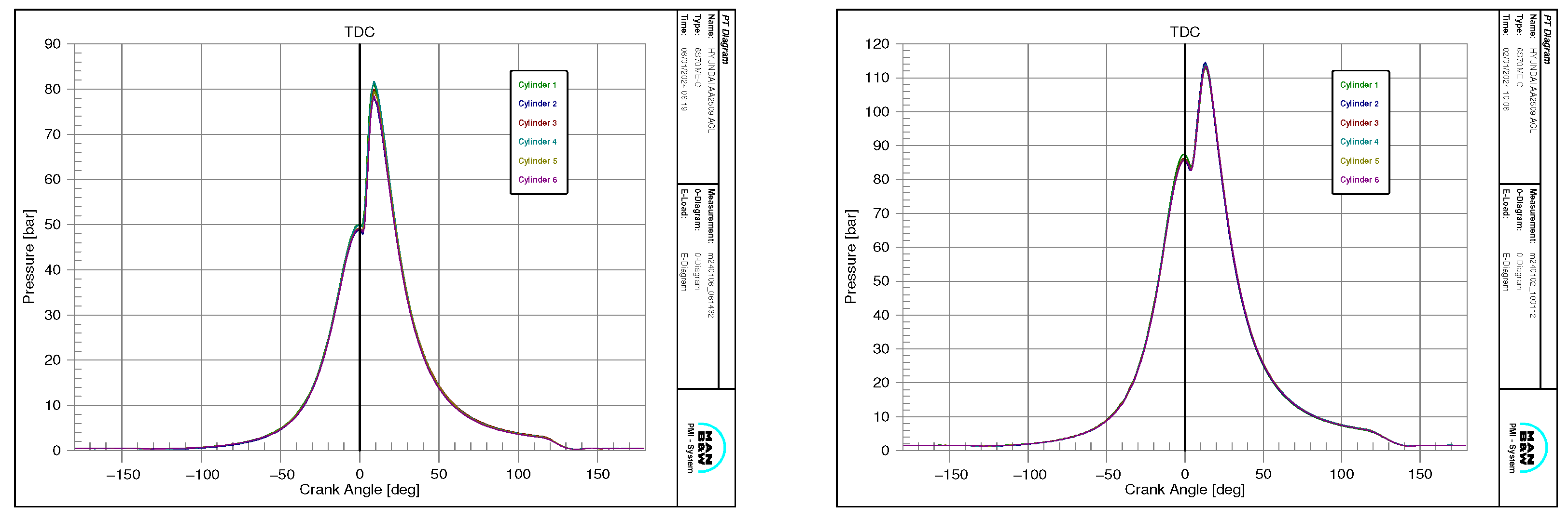Engine load is calculated as the ratio of the current whole engine effective power to the engine power at MCR, which is equal to 17,550 kW, according to Table 1. The indicated pressure curves for the starboard main engine in each cylinder are presented below in Figure 2.

In addition to this, the data was used to generate synthetic data in three ways. The first set was generated solely from the port data, while the second set was generated using only the starboard data. The combined dataset was created by randomly mixing the port and starboard datasets to create a dataset double the original size (38 data points in total). These were then used to generate three synthetic datasets, each numbering 500 newly generated data points. The technique used for generating this data is described in the next subchapter. The original datasets were used for the verification of the scores. Although this does introduce the possibility of overfitting to the original data due to it being used both as the synthetic source and the validation tool for the regression models, it must be noted that the synthetic data is newly generated and, while it follows the same statistical distributions as the original data, it does not contain the same points. This means that rough overfitting, where the model learns the data points directly, should be avoided, although it can be expected that some overfitting will be present in the range of data used as a source; this means the models may have poorer performance if they should be validated on a wider range of data (e.g., higher loads). Still, as this data is not available and the total amount of data is limited, this is the most valid approach, as testing using part of the already small dataset would reduce the sample size to the point of unusability.

Copulagan Data Generation Technique

The CopulaGAN algorithm is a hybrid generative framework designed for synthesizing realistic tabular data, particularly in scenarios where both continuous and categorical variables coexist and where feature dependencies are nontrivial [16]. Its architecture integrates two core components: a statistical copula model for transforming real data into a structured latent space and a generative adversarial network (GAN) trained in that space to learn and replicate the joint distribution of the transformed features [17]. The use of copulas is critical, as it enables the modeling of complex multivariate dependencies independent of marginal distributions; this principle overcomes one of the fundamental limitations of vanilla GANs when applied to tabular datasets [18]. By first separating the dependency structure (captured by a copula) from the marginals, CopulaGAN ensures that both aspects of the data distribution are preserved and reproducible through synthesis [19]. CopulaGAN was selected based on the preliminary tests between four methods: itself, pure GaussianCopula, Conditional Tabular GAN, and Tabular Variable Autoencoder. The methods were run for a fewer number of epochs (approx. 1000) to determine their performance, with CopulaGAN showing the most promising results.

Formally, given a dataset $X={[x^{\left(1\right)},x^{\left(2\right)},\dots ,x^{\left(n\right)}]}^{\top }\in {\mathbb{R}}^{n\times d}$ with n samples and d features, each column $x_j$ is transformed to the unit interval via its marginal cumulative distribution function (CDF) $F_j$, resulting in $u_j=F_j\left(x_j\right)$ for all $j\in \{1,\dots ,d\}$. This yields a new dataset $U={[u^{\left(1\right)},u^{\left(2\right)},\dots ,u^{\left(n\right)}]}^{\top }$, where each $u^{\left(i\right)}\in {[0,1]}^d$, and the marginal distribution of each feature is approximately uniform over $[0,1]$:

$$u_j^{\left(i\right)}=F_j\left(x_j^{\left(i\right)}\right),\forall i\in \{1,\dots ,n\},j\in \{1,\dots ,d\}.$$

(1)

The motivation for this transformation stems from Sklar’s Theorem, which states that any multivariate joint distribution $H(x_1,\dots ,x_d)$ can be decomposed into its marginals and a copula C that captures their dependency structure:

$$H(x_1,\dots ,x_d)=C(F_1\left(x_1\right),\dots ,F_d\left(x_d\right)),$$

(2)

where $C:{[0,1]}^d\to [0,1]$ is a copula function encoding the joint dependence. This decomposition allows the learning process to be split into two stages: modeling the marginals (which are handled deterministically via empirical CDFs or kernel estimators) and modeling the copula (i.e., the dependency structure) using a GAN [20].

In the second stage, a generative adversarial network is trained to model the empirical distribution of the transformed dataset U. The GAN consists of a generator function $G:{\mathbb{R}}^k\to {[0,1]}^d$ and a discriminator $D:{[0,1]}^d\to [0,1]$. The generator receives random noise vectors $z\sim \mathcal{N}(0,I_k)$ as input and outputs synthetic samples $u^{\prime }=G\left(z\right)$ that aim to mimic the distribution of real samples $u\in U$. The discriminator attempts to distinguish between true samples from U and synthetic samples from G. The adversarial training objective is formulated as a minimax game [21]:

$$\underset{G}{min}\underset{D}{max}{\mathbb{E}}_{u\sim P_U}[logD\left(u\right)]+{\mathbb{E}}_{z\sim \mathcal{N}(0,I_k)}[log(1-D\left(G\left(z\right)\right))],$$

(3)

where $P_U$ denotes the empirical distribution of the copula-transformed dataset. Through iterative updates using stochastic gradient descent, the generator learns to produce samples that the discriminator cannot reliably distinguish from the real ones, thereby approximating $P_U$ [22].

Once training converges, synthetic data generation proceeds by sampling a latent vector z, applying the generator to obtain a synthetic copula sample $u^{\prime }=G\left(z\right)$, and then applying the inverse CDFs $F_j^{-1}$ to each feature to map the data back to the original domain. For continuous features, the inverse transformation is given by [23]:

$$x_j^{\prime }=F_j^{-1}\left(u_j^{\prime }\right),\forall j\in \{1,\dots ,d\},$$

(4)

yielding a synthetic dataset $X^{\prime }={[x^{\prime \left(1\right)},x^{\prime \left(2\right)},\dots ,x^{\prime \left(n\right)}]}^{\top }$ that mimics the statistical properties of the original data X in terms of both marginal distributions and feature correlations [20]. For categorical variables, the GAN operates on embedded representations during training, and an inverse transformation (e.g., Gumbel-softmax decoding) is used to project the continuous outputs back into discrete categories [24].

An essential strength of CopulaGAN is its ability to model non-Gaussian, nonlinear dependencies between variables without explicitly assuming any parametric form for the joint distribution. This makes it particularly well-suited for high-dimensional, heterogeneous data, where variable relationships may be complex and poorly captured by classical multivariate distributions such as multivariate Gaussians or mixtures of Gaussians [24]. Additionally, because the GAN operates in a normalized space with uniform marginals, it avoids common training instabilities that arise when learning directly from highly skewed or mixed-type feature spaces [25].

To ensure high-quality synthesis and prevent issues such as mode collapse or overfitting, CopulaGAN incorporates additional regularization strategies and stabilization techniques during training. These include batch normalization, label smoothing, and optionally gradient penalties, particularly if a Wasserstein GAN formulation is used instead of the vanilla binary cross-entropy objective [26]. The final synthetic data can be evaluated through a combination of statistical similarity metrics (e.g., marginal KS statistics and correlation distance) and task-based metrics, such as classifier fidelity or downstream prediction consistency [22,27]. To ensure that the data makes physical sense, the ranges of certain values (e.g., RPM in terms of the load) are fixed, ensuring that only the appropriate values are generated. While this should hold even without this intervention, as the method should generate statistically sensible data, it is checked once more for assurance after the synthetization.

3. Multilayer Perceptron Regression

Multilayer perceptron (MLP) represents a class of feedforward artificial neural networks composed of multiple layers of nodes, where each layer is fully connected to the next [28]. It is one of the fundamental architectures in deep learning and forms the basis for many modern neural models across classification, regression, and function approximation tasks [29]. The MLP is characterized by its layered structure, comprising an input layer that receives the raw features, one or more hidden layers that perform nonlinear transformations, and an output layer that produces the final prediction. Each node (or neuron) in a hidden or output layer computes a weighted sum of its inputs, adds a bias term, and passes the result through a nonlinear activation function to introduce expressive capacity into the model [30].

Formally, consider an input vector $x\in {\mathbb{R}}^d$ with d features. In an MLP with L layers (excluding the input), the computation proceeds through successive transformations. Each layer ℓ is associated with a weight matrix $W^{(\ell )}\in {\mathbb{R}}^{n_{\ell }\times n_{\ell -1}}$ and a bias vector $b^{(\ell )}\in {\mathbb{R}}^{n_{\ell }}$, where $n_{\ell }$ denotes the number of neurons in layer ℓ. The input to the first hidden layer is computed as [31]:

$$h^{\left(1\right)}=\varphi \left(W^{\left(1\right)}x+b^{\left(1\right)}\right),$$

(5)

where $\varphi (·)$ is a nonlinear activation function, such as ReLU, sigmoid, or tanh. The subsequent layers apply similar transformations [31]:

$$h^{(\ell )}=\varphi \left(W^{(\ell )}{h}^{(\ell -1)}+b^{(\ell )}\right),\forall \ell \in \{2,\dots ,L-1\}.$$

(6)

The output layer computes

$$\widehat{y}=f_{\mathrm{out}}\left(W^{\left(L\right)}{h}^{(L-1)}+b^{\left(L\right)}\right),$$

(7)

where $f_{\mathrm{out}}(·)$ is the output activation function, typically chosen according to the nature of the learning task. For classification problems, a softmax activation is used to obtain class probabilities, while for regression, the output is often left as linear [32].

A key property of MLPs is their ability to approximate arbitrary continuous functions given sufficient network width and depth—a result known as the universal approximation theorem. This is achieved through the composition of affine transformations and nonlinear activation functions, allowing the network to learn complex, nonlinear mappings from inputs to outputs [33]. However, while shallow MLPs can theoretically approximate any function, deeper architectures are often required in practice to efficiently represent highly nonlinear functions without exponentially increasing the number of neurons [34].

MLP is trained using supervised learning techniques, most commonly by minimizing a task-specific loss function through backpropagation and gradient-based optimization. In regression tasks, the mean squared error (MSE) loss is typically used [35]:

$${\mathcal{L}}_{\mathrm{MSE}}={\displaystyle \frac{1}{N}}\sum _{i=1}^N{({\widehat{y}}_i-y_i)}^2,$$

(8)

where N is the number of training samples, ${\widehat{y}}_i$ is the network prediction, and $y_i$ is the ground truth value for sample i [36].

Backpropagation computes the gradient of the loss function with respect to each network parameter using the chain rule, allowing for the efficient computation of updates for all layers simultaneously. These gradients are then used to adjust the weights via stochastic gradient descent (SGD) or its variants, such as Adam, to minimize the loss over the training dataset [37].

The design choices in an MLP—including the number of hidden layers, the number of units per layer, the type of activation function, and the choice of optimizer and learning rate—play a crucial role in determining the network’s ability to learn from data and generalize to unseen inputs. These hyperparameters are typically selected via grid searches based on performance on a validation set [38].

To optimize model performance and ensure generalization, an exhaustive grid search was performed across a well-defined hyperparameter space (

Table 3. Grid search hyperparameter space for MLP models.

Hyperparameter	Values Considered
Hidden layer sizes	(10), (50), (100), (10, 10), (50, 50), (100, 100),
	(10, 10, 10), (50, 50, 50), (100, 100, 100),
	(10, 10, 10, 10), (50, 50, 50, 50), (100, 100, 100, 100)
Activation function	identity, logistic, tanh, ReLU
Solver	lbfgs, Adam
Regularization parameter $\alpha$	0.0001, 0.001, 0.01, 0.1
Learning rate strategy	constant, adaptive
Initial learning rate	0.01, 0.1, 1

). This search covered various architectural configurations, including shallow and deep multilayer perceptron (MLP) structures, activation functions, solvers, regularization coefficients, and learning rate strategies. Specifically, 12 different hidden layer topologies were considered, ranging from single-layer networks (e.g., (10), (50), (100)) to deeper networks with up to four hidden layers (e.g., (100, 100, 100, 100)). Each architecture was evaluated under four activation functions—identity, logistic, tanh, and ReLU—and two optimization solvers: the quasi-Newton lbfgs and the adaptive gradient-based Adam algorithm [39].

To account for overfitting and model variance, a five-fold cross-validation procedure was employed during the grid search. The dataset was partitioned into five equally sized folds. For each hyperparameter combination, the model was trained on four folds and validated on the remaining fold. This process was repeated five times, with each fold serving as the validation set once, and the results were averaged to obtain robust estimates of generalization performance [40]. The evaluation criterion for selecting the best model was the minimization of the mean absolute percentage error (MAPE) on the validation folds. This approach ensures that the selected models generalize well and are not biased by specific partitions of the training data [41,42].

Training using the above hyperparameters was performed using a single node consisting of a Intel (Santa Clara, CA, USA ) Xeon E5 processor with 24 nodes/48 threads at 3.50 GHz, with 64 GB of RAM. The training time using this hardware was approximately 18 h per each of the tested cases. Although MLPs have largely been superseded by more specialized architectures in domains such as image and sequence modeling (e.g., CNNs and RNNs), they remain highly effective models for tabular data, function approximation, and settings where the input features have no inherent spatial or temporal structure [43].

MLP was selected as the regression technique based on previous research in the field [4,5] and the state-of-the-art review, which shows that it is the most popular method, used in almost all of the reviewed research as either one of the tested methods (in which case, it is usually the best performing one) or the main method used.

Evaluation

Two metrics were used to evaluate the scores in this study. For the evaluation of the regression scores, the mean absolute percentage error (MAPE) metric was used, while the column pair score was used to evaluate synthetization quality.

The MAPE is a widely used metric for evaluating the accuracy of regression models, particularly when the interpretability of errors in relative terms (percentages) is desired. MAPE expresses the average absolute deviation between the predicted and true values as a percentage of the true values, making it scale-independent and suitable for comparisons across datasets with varying magnitudes [44].

Given a set of N true values $y_i$ and corresponding model predictions ${\widehat{y}}_i$, MAPE is defined as

$$\mathrm{MAPE}={\displaystyle \frac{100\%}{N}}\sum _{i=1}^N\left|{\displaystyle \frac{y_i-{\widehat{y}}_i}{y_i}}\right|,$$

(9)

where the absolute percentage error is computed for each instance and then averaged over all instances in the dataset. The multiplication by $100\%$ converts the result into a percentage.

The Column Pair Distance Score is a metric used primarily for evaluating the quality of synthetic tabular data. It quantifies the preservation of pairwise dependencies (typically correlations or mutual information) between features in the synthetic dataset relative to the original dataset. A high column pair score indicates that the synthetic data closely replicates the interfeature relationships of the real data [45].

Let $X_{\mathrm{real}}\in {\mathbb{R}}^{n\times d}$ and $X_{\mathrm{synthetic}}\in {\mathbb{R}}^{m\times d}$ denote the real and synthetic datasets, respectively, each with d features. For each pair of columns $(i,j)$, a dependence measure—commonly the Pearson correlation coefficient ${\rho }_{ij}$—is computed:

$${\rho }_{ij}^{\mathrm{real}}={\displaystyle \frac{\mathrm{Cov}(X_{\mathrm{real}}^{\left(i\right)},X_{\mathrm{real}}^{\left(j\right)})}{{\sigma }_{X_{\mathrm{real}}^{\left(i\right)}}·{\sigma }_{X_{\mathrm{real}}^{\left(j\right)}}}},{\rho }_{ij}^{\mathrm{syn}}={\displaystyle \frac{\mathrm{Cov}(X_{\mathrm{synthetic}}^{\left(i\right)},X_{\mathrm{synthetic}}^{\left(j\right)})}{{\sigma }_{X_{\mathrm{synthetic}}^{\left(i\right)}}·{\sigma }_{X_{\mathrm{synthetic}}^{\left(j\right)}}}}.$$

(10)

The pairwise score is then calculated as the average absolute difference in the selected dependency measure across all unique column pairs:

$$\mathrm{Column}\mathrm{Pair}\mathrm{Distance}={\displaystyle \frac{2}{d(d-1)}}\sum _{i=1}^{d-1}\sum _{j=i+1}^d\left|{\rho }_{ij}^{\mathrm{real}}-{\rho }_{ij}^{\mathrm{syn}}\right|.$$

(11)

To convert this distance into a similarity score (where higher values are better), it is common to define the column pair score as

$$\mathrm{Column}\mathrm{Pair}\mathrm{Score}=1-\mathrm{Column}\mathrm{Pair}\mathrm{Distance}.$$

(12)

This metric ranges from 0 to 1, where a score of 1 indicates perfect preservation of all pairwise dependencies between the real and synthetic datasets.

4. Results and Discussion

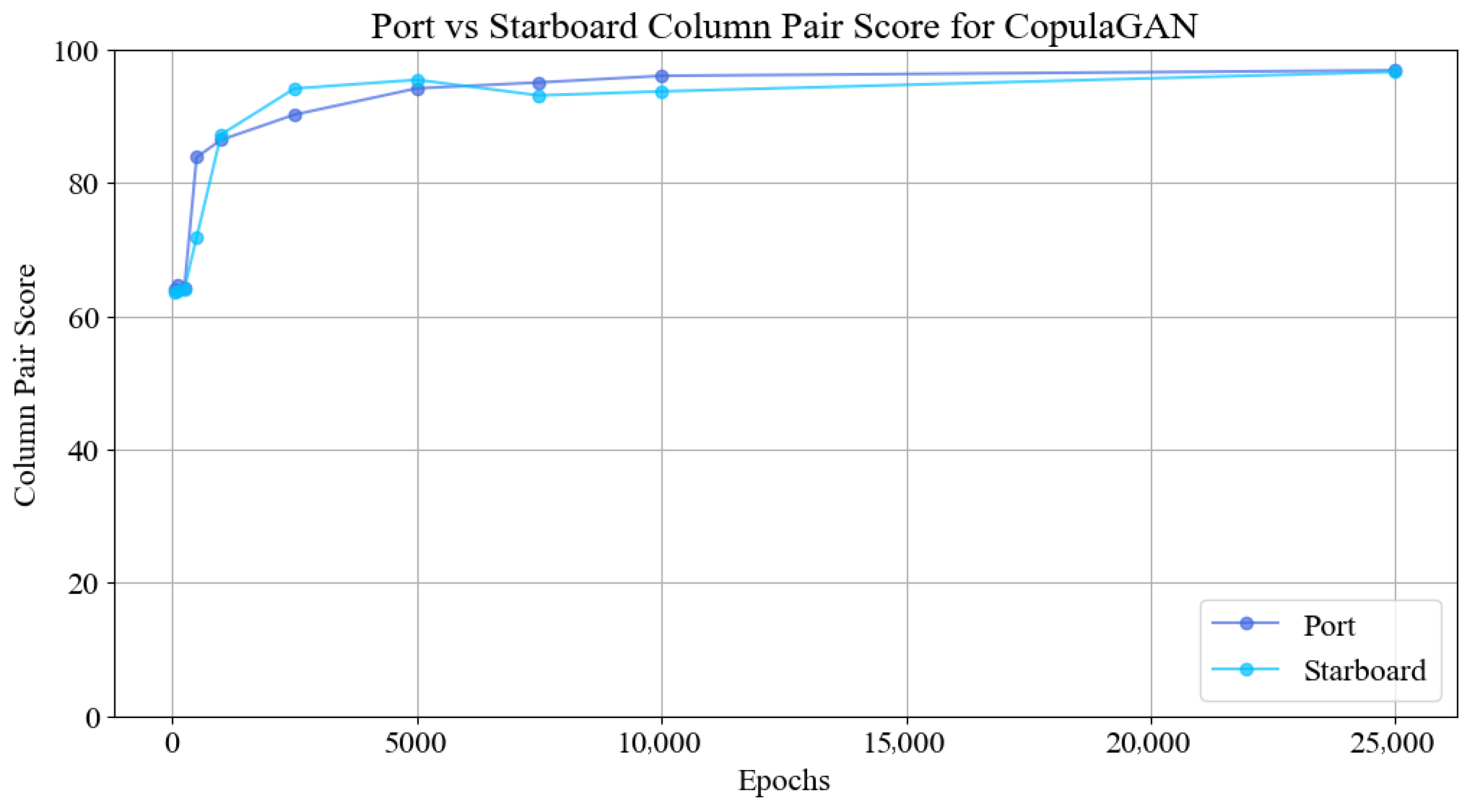
Figure 3 presents the evolution of the column pair score as a function of the number of training epochs for the CopulaGAN model. Two separate datasets, denoted port and starboard, were evaluated independently to assess the consistency and stability of the generative process across structurally similar yet statistically distinct inputs. The x-axis represents the training duration in epochs, ranging from 0 to 25,000, and the y-axis indicates the column pair score, scaled between 0 and 100, which represents the degree of preservation of pairwise statistical dependencies in the synthetic data relative to the original dataset.

As shown in the figure, both datasets exhibit a rapid increase in score within the first few thousand epochs, indicating that the model quickly learns the essential inter-feature dependencies. Initially, at epoch 0, the scores are relatively low (approximately 64 for port and 65 for starboard), reflecting poor pairwise structure in the untrained model. However, by 1000 epochs, the scores improve significantly, reaching values above 85 for both datasets. Notably, the starboard dataset achieves slightly higher performance earlier in the training, peaking near 96 at around 5000 epochs; this suggests that its structural dependencies may be more learnable under the same model configuration.

Beyond 5000 epochs, the score curves begin to plateau, with only marginal gains observed. This behavior implies that the majority of structural learning occurs in the early training stages and that extending training beyond 10,000 epochs yields diminishing returns in terms of pairwise fidelity. The final scores, recorded at 25,000 epochs, are nearly identical for both datasets, converging to values just below 98, indicating excellent structural consistency in the generated synthetic data for both subsets.

In the following figures, the regression model scores for the engine efficiency, fuel consumption, engine load, and engine power of the port and starboard engines are given. All four of these outputs have been modeled using synthetic data based on the combination of two datasets: synthetic data derived solely from the port engine measurements and synthetic data derived solely from the starboard engine measurements. All of the values are expressed as percentage errors (MAPE).

Figure 4 demonstrates the model scores targeting the port data values. Engine load prediction is the poorest overall, ranging from 7.62% to 19.25% across targets. For the values of efficiency, the best score is achieved using the model trained using the synthetic data generated from the combination of both datasets. The same is true for fuel usage. Interestingly, power prediction is the best when using the model trained on the starboard engine. Still, both of the models trained on data synthesized from port data and combined data have achieved satisfactory performance on this target (1.98% and 2.70%). The same holds for the other targets, where the ranges of errors across different input data are low enough that all of them could be considered successful—except for engine load prediction, which may be considered unsatisfactory due to an error of more than 5%.

For the port dataset, the MAPE results show relatively strong predictive performance across all target variables on the training dataset. In the continuation of this paragraph, the values of the best hyperparameters for selected models, along with their performance during the grid search training procedure, are given. The efficiency model yielded an average MAPE of 8.4%, with a standard deviation of 3.25% across cross-validation folds. This model used a neural network with a tanh activation function, two hidden layers of 50 neurons each, a constant learning rate with an initial value of 0.1, an ${\ell }_2$ regularization parameter $\alpha$ of 0.001, and training using the Adam optimizer. For power, the MAPE was 5.6% on average, with a standard deviation of 14.07%. This model employed a simpler architecture, consisting of a single hidden layer of 50 neurons, an identity activation function, and the same constant learning rate initialization (0.01), using the Adam optimizer with a regularization strength of $\alpha =0.0001$. Load prediction was the most accurate, with an average MAPE of 0.79% and a standard deviation of 0.26%. This model used three hidden layers of 100 neurons each, the tanh activation function, and $\alpha =0.01$, and it was optimized using the L-BFGS solver with a relatively aggressive learning rate of 1.0. Lastly, the fuel prediction model had an average MAPE of 1.72% and a standard deviation of 0.981%. It used two hidden layers of 250 neurons each, the identity activation function, an adaptive learning rate strategy initialized at 0.1, and an $\alpha$ value of 0.1, trained using Adam. These results are shown in Figure 4.

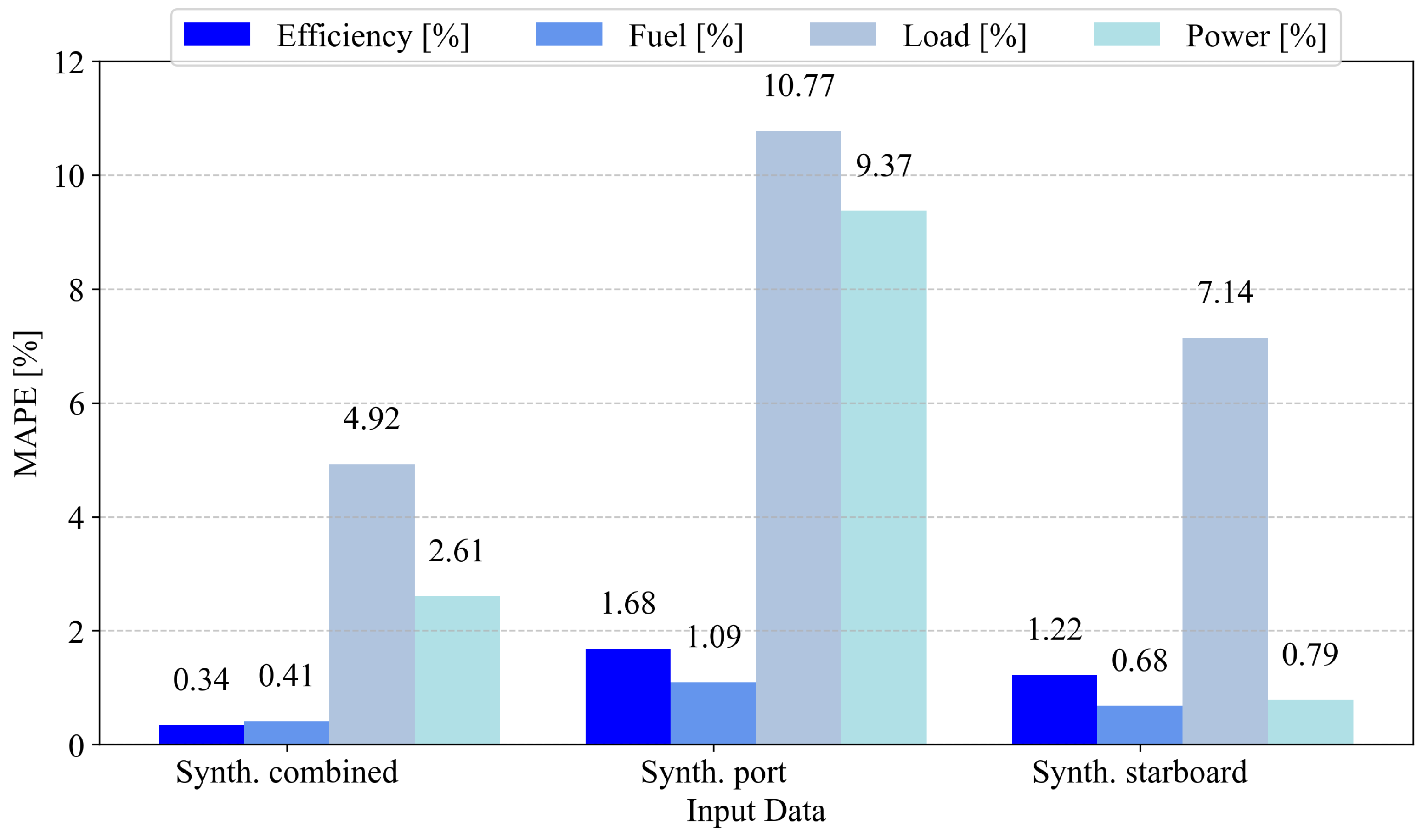
In the case of the starboard engine values being targeted, a lot of similarities exist, as can be seen in Figure 5. First, when observing engine efficiency, we can see that the lowest error of 0.34% is achieved using the model trained on the dataset synthesized from the two combined datasets. This is much lower compared to the 1.68% value obtained using the model trained on synthesized port data and the 1.22% value from the model trained on the synthesized starboard data. The case of fuel usage is similar, where the model trained on the combined synthesized dataset achieved the lowest error at 0.41%, compared to 1.09% and 0.68% for the models trained on the port and starboard synthesized data. Unlike before, where all three models achieved satisfactory scores for the engine power metric, the model trained on port data had a significant error of 9.37%, compared to 2.61% from the model trained on the combined data and 0.79% from the starboard data. Engine load is once again shown to be difficult to predict with the available data, with the lowest error rate of nearly 5% for the model trained on the combined dataset.

As before, the values of the training scores and hyperparameters for the selected models on the starboard dataset are described going forward. The results are comparable but exhibit slightly higher error variance. The efficiency model showed an average MAPE of 6.6%, with a fold-wise standard deviation of 3.38%. This model used a deeper architecture with three hidden layers of 500 neurons each and tanh activation. It adopted a constant learning rate of 0.01, with $\alpha =0.1$, optimized via Adam. Power prediction showed excellent performance, with an average MAPE of just 0.81% and a very low standard deviation of 0.807%. It used four hidden layers of 10 neurons each, the ReLU activation function, a constant learning rate initialized at 0.01, and $\alpha =0.01$, trained using Adam. The load model exhibited a higher MAPE of 2.11%, with a standard deviation of 0.369%. It used two hidden layers of 100 neurons each, with tanh activation, an adaptive learning rate initialized at 0.1, and a regularization strength of 0.1. Finally, the fuel model had an average MAPE of 1.63% and a low standard deviation of 0.21%. It was based on a single-layer network with 50 neurons, the logistic activation function, a constant learning rate of 0.01, and $\alpha =0.01$, trained using Adam.

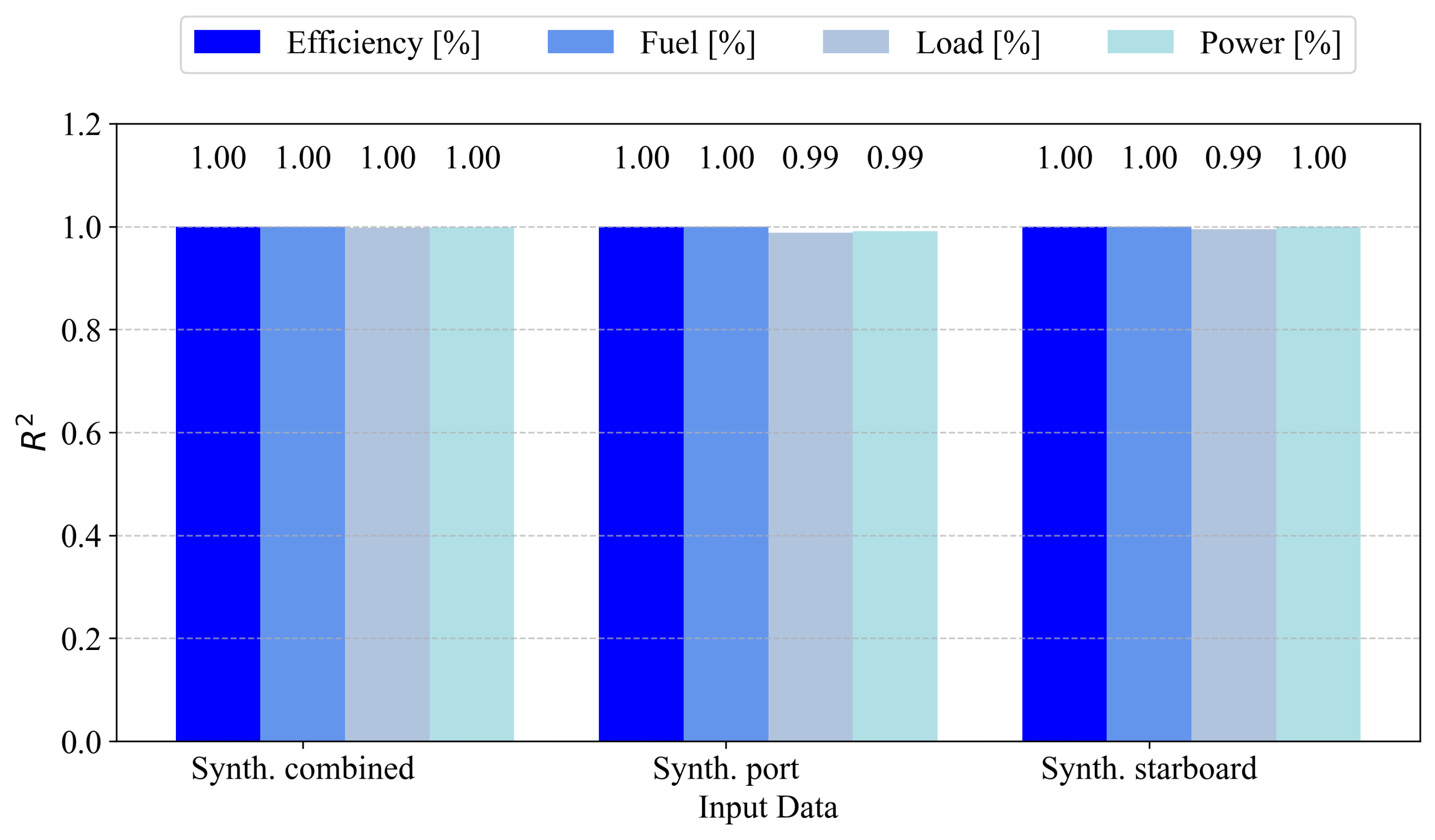
To facilitate easier comparison with other state-of-the-art results, the coefficient of determination for both the starboard and port models is presented. First, Figure 6 illustrates the coefficient of determination ($R^2$) for the starboard engine. All variables under the Synth. combined configuration achieved an $R^2$ of 1.00, indicating perfect correlation with the actual values. The Synth. port configuration exhibits perfect performance for efficiency and fuel ($R^2=1.00$), while load and power are marginally lower at 0.99. A similar trend is observed for Synth. starboard, with efficiency, fuel, and power maintaining an $R^2$ of 1.00, while load is slightly lower at 0.99. These results demonstrate the high predictive fidelity of models trained on synthetic data, with negligible degradation in explained variance.

Figure 7 presents the $R^2$ values for the models trained on the synthetic data derived from the port engine. All performance indicators—efficiency, fuel, load, and power—achieve near-perfect predictive accuracy. Both efficiency and fuel reach an $R^2$ of 1.00 across all input types. Power also consistently attains a value of 1.00, while load exhibits slightly reduced values of 0.99 with the Synth. combined and Synth. port inputs and 0.96 with the Synth. starboard input. These results suggest strong generalization for port engine predictions, with only minor degradation observed in load estimation when using starboard-derived synthetic data.

All models exhibit high performance when the $R^2$ metric is observed, with all of the models having values greater than 0.95 and most having a value of 1.00 when rounded to two significant digits. Still, the much poorer results for the MAPE metric indicate that not all of the models are appropriate; however, since no $R^2$ measures were poor for any of the models, we can conclude that the models that did satisfy the MAPE scores are satisfactory.

The acceptable error indicates the highest error that the model can have when tested on original data (scores provided in Figure 4 and Figure 5). Based on the standard acceptable errors in the field, the acceptable MAPE can be set to 2%. With this in mind, we can conclude that the port side’s engine efficiency can be targeted using any input data, which also applies to fuel consumption. The port’s engine power can be targeted using any inputs except combined synthetic data. In contrast, the load of the port-side engine cannot be targeted using any inputs, as all models achieve an error that is much higher than acceptable. For the starboard side, again, efficiency and fuel consumption are acceptable across all inputs; however, this is not the case for load and power. The load models have failed to converge to an acceptable solution, similar to the case of the port side engine. However, the only acceptable input for power was the synthetic data generated from the starboard engine’s data, resulting in a MAPE of 0.79%.

5. Conclusions

This study utilized a small dataset as the source for generating synthetic data. The CopulaGAN approach, trained for up to 25,000 epochs, was applied to the original data to generate 500 values based on the data collected from the starboard engine, 500 values based on the data collected from the port engine, and 500 values based on a mix of the two. The original datasets, which constitute 19 data points each, were not used again until the validation process.

The scores, in general, are satisfactory, with at least one approach per engine output yielding a satisfying score. The only exception is the engine load, which had the highest errors in the data used in this study. Beyond that, other metrics achieved satisfactory scores, with the efficiency of the port-side engine having an error of only 0.50% when using a model trained on combined synthetic data. The same data was used to achieve a low error of 0.70% for the fuel consumption model. Interestingly, the effective power metric of the port-side engine had the lowest error when modeled using the starboard-data-based model. In other words, the additional information in that data helped achieve a lower score in that instance. This cross-modeling was not the case for the starboard version, where the model trained on the port data had an extremely high error (9.37%) compared to the model trained on the starboard data (0.79%). The combined data-driven model was again the best for engine efficiency and fuel consumption, with errors of only 0.34% and 0.41%, respectively.

Finally, we address the research questions posed at the start of this article:

• (RQ1) For the given case, the model trained only on synthetic data can provide good performance when real-world data is used for training;
• (RQ2) Cross modeling can be applied to a degree, but the models for different aspects of individual engines still generally achieved the best scores when modeled using their respective data or combined data, as noted in (RQ3);
• (RQ3) The combination of both sets of data tends to have the best results when used as source data for synthetic data used to train models, at least in the cases of mechanical efficiency and fuel consumption.

One of the main limitations of this paper is that the data was only recorded at lower engine loads (<60%). This is the most likely cause of the high error in the regression of the current engine load values. Due to the low amount of repeating data, it is better to remove this value or collect additional data points. Training it as a classification task in this particular case may also prove to be useful. Additionally, it is worth noting that the amount of original data was extremely limited. This is why the authors were unable to split the dataset and used it both as a source and validation set. Although this should not have a significant impact, it is worth noting. Another manner in which additional validation could have been performed is by testing the predicted values on the set of engines at different operating parameters. Sadly, the engines were unavailable for additional validation measurements after data collection, which is why the data was validated strictly based on the data collected prior to the study. Unlike conventional models, the ML approach has certain drawbacks; however, the general methodology can be applied to different marine engines, but the full training process needs to be repeated, from data synthesis to data training. While direct application may be possible for similar engines and different loads, it could not be recommended without at least a validation run. The lack of cross-comparison between different methods, such as gradient-boosted or support vector machines, is a notable limitation of this study. It must be noted that the goal of the presented paper was to demonstrate the possibility of performing the modeling in the presented environment (scarce data outside of the commonly used load ranges), and we are planning on further expanding it in future work. Future work will also focus on improving the achieved score, as well as collecting additional data to enhance the quality of validation.