A Design of Leaderless Formation Controller for Multi-ASVs with Sampled Data and Communication Delay

Abstract

The formation control technology of the multi-ASV (autonomous surface vehicle) system is one of the key technologies required for performing maritime missions. In this paper, a leaderless formation controller is proposed, where the issues of sampled communication and data transmission delays in formation are taken into consideration. By introducing the desired displacements and the implicit formation center (IFC), the control goal of the leaderless formation is explicitly defined. Through the application of a state-space transformation, the achievement of the leaderless formation is shown to be equivalent to the stabilization of the transformed subsystem. The implicit formation center of the leaderless framework is derived, which facilitates the description and analysis of formation movements. The stability of the system is rigorously analyzed by using the Lyapunov–Krasovskii functional. Furthermore, an $H_{\infty }$ performance controller is designed to evaluate the tolerance of the leaderless formation against marine environmental disturbances. Numerical simulations with 10 ASVs under sampled communication and transmission delay demonstrate the effectiveness of the proposed controller, achieving an $H_{\infty }$ performance bound $\gamma$ of 10.

1. Introduction

Autonomous surface vehicles (ASV) are vessels equipped with sensors, navigation algorithms, and communication systems, enabling them to operate on the surface either fully autonomously or semi-autonomously. These platforms have emerged as indispensable assets in maritime operations owing to their remarkable versatility and operational efficiency [1]. Widely used in surface cleaning [2], environmental monitoring [3], emergency response operations [4], and offshore resource exploration, ASVs provide safer, more cost-effective and efficient alternatives to traditional manned vessels [5]. Their ability to operate in hazardous or remote environments without endangering human lives has made them indispensable for numerous critical applications. Moreover, the rapid advance in artificial intelligence, control systems, and sensor technologies has significantly improved the capabilities of ASVs, enabling them to perform increasingly complex and autonomous tasks [6].

In recent years, growing interest in multi-agent systems has spurred substantial progress in the collaborative operation of unmanned vehicles [7], including unmanned aerial vehicles and autonomous ground vehicles [8,9,10,11]. Similarly, multi-ASVs have demonstrated significant potential in collaborative missions, working together to accomplish tasks such as large-scale environmental monitoring, cooperative target tracking, and distributed data collection [12,13]. However, operating in dynamic and highly uncertain marine environments presents ASVs with unique challenges in communication, coordination, and control [14,15]. These challenges have become a driving force for research into advanced collaborative strategies for multi-ASV systems, aiming to enhance their effectiveness and reliability in real-world maritime applications [16].

Among the various collaborative strategies for the multi-ASV system, formation control has emerged as a cornerstone to allow coordinated operations [17]. Formation control refers to the ability to regulate ASVs to maintain a desired geometric configuration while collectively achieving mission objectives. It enables the team to perform complex operations in dynamic marine environments, such as formation path following and coordinated encirclement, while addressing disturbances and communication constraints with robust coordination strategies [18,19,20,21]. From the perspective of controller design, a variety of control algorithms have been developed for multi-ASV formation. For example, Li et al. proposed a neural network PID controller, which benefits from the simplicity and adaptability of PID control but may face challenges in handling strong nonlinearities and time delays [22]. Zhou et al. introduced an adaptive fuzzy backstepping-based controller to deal with unknown nonlinearities and actuator saturation, improving robustness but increasing the complexity of parameter tuning [23]. Wang et al. presented an adaptive second-order fast terminal sliding-mode controller, which offers strong robustness against disturbances and uncertainties, though it may suffer from chattering and implementation complexity [24]. Moreover, the successful application of PID controllers based on adaptive neuro-fuzzy inference systems in robotic gripper systems [25,26,27] provides useful insights for the development of intelligent and robust cooperative control strategies for multi-ASVs. In addition, recent nature-inspired optimization algorithms, such as the polar fox optimization algorithm [28,29], have demonstrated strong performance in solving complex, high-dimensional optimization problems by simulating the adaptive hunting behaviors of polar foxes.

Beyond controller design, structural strategies such as the leader–follower and virtual structure methods have also played a pivotal role in the development of formation maintenance approaches. These early methods laid important foundations by assigning predefined roles or enforcing geometric constraints among ASVs [30,31]. The leader–follower method relies on explicitly designated leaders as references, making implementation straightforward but rendering the formation vulnerable to the leader’s performance. The virtual structure method, which models the entire formation as a rigid body, allows for precise geometric control but struggles to adapt to dynamic changes such as obstacle avoidance or member reconfiguration. Both methods depend on explicit reference points—either a leader or a virtual structure—which can limit flexibility and robustness in highly dynamic or uncertain environments [32,33].

The aforementioned limitations have motivated the development of leaderless formation control approaches, which eliminate explicit leadership or centralized references [34,35,36]. For example, Zhang et al. designed an auxiliary variable to transform the formation control problem into a consensus problem, enabling ASVs to achieve formation without a leader [34]. Hu et al. proposed a distributed leaderless encirclement algorithm, allowing ASVs to autonomously form a convex hull around a target, thus improving the scalability and adaptability of the formation [36]. In addition, considering practical constraints such as non-continuous communications and electromagnetic interference, Yu et al. introduced a dynamic event-triggered communication scheme that reduces communication load by only transmitting data when necessary [37]. Wang et al. further addressed communication delays by modeling the containment maneuvering problem as a time-delay system and designing consensus protocol parameters to mitigate the impact of delays [38]. These developments serve as the key motivation for our study on leaderless formation under sampled communication and transmission delays. In addition, the consideration of environmental disturbances—such as wind, waves, and ocean currents—is crucial for real-world multi-ASV applications. Disturbance attenuation becomes even more important in leaderless formations, where no explicit leader provides a central reference and each ASV must autonomously reject external influences. The $H_{\infty }$ control approach, which has been widely employed for enhancing disturbance rejection in single-ASV systems [39,40], offers a systematic framework to address such challenges in multi-ASV formation control. To clarify the differences between existing approaches and our proposed method,

Table 1. Comparison of representative formation control works.

Works	Formation Framework	Communication Mode	Delay Assumption
Zhang et al. [34]	Leaderless framework	Event-triggered communication	No delay
Hu et al. [36]	Leaderless framework	Continuous communication	No delay
Yu et al. [37]	Leader–follower framework	Event-triggered communication	No delay
Wang et al. [38]	Leader–follower framework	Continuous communication	Time-varying delay
Proposed Method	Leaderless framework	Aperiodic sampled communication	Fixed delay

presents a comparative overview.

To address the challenges posed by the leader–follower framework, non-ideal communication, and marine environmental disturbances in multi-ASV formations, the main objectives and contributions of this paper are as follows:

1.

Sampled-data delay-aware formation control: We design a formation controller that explicitly accounts for aperiodic sampled communication and transmission delays, in contrast to existing methods that assume continuous communication [41,42].

2.

Leaderless framework with implicit formation center (IFC): We propose a leaderless formation control method and derive the trajectory of the IFC to characterize group motion. This approach differs fundamentally from traditional leader–follower schemes [43,44].

3.

$H_{\infty }$ performance against disturbances: We further design a leaderless formation controller that ensures a specified disturbance attenuation level against marine environmental disturbances using $H_{\infty }$ norm analysis.

The remainder of this paper is organized as follows. Section 2 introduces the system model and formally states the problem. Section 3 presents the design of the leaderless formation controller and the theoretical analysis of system stability. Section 4 provides simulation results to demonstrate the effectiveness of the proposed approach. Finally, Section 5 concludes the paper and outlines future research directions.

Notation. 

To ensure clarity in the expressions, several specific mathematical symbols are defined as follows. ${\mathbb{R}}^n$ and ${\mathbb{R}}^{n\times m}$ denote the n-dimensional Euclidean space and the space of $n\times m$ real matrices, respectively. The n-dimensional identity matrix is represented by ${\mathbf{I}}_n$, while ${\mathbf{0}}_{n\times m}$ and ${\mathbf{1}}_{n\times m}$ refer to $n\times m$ matrices filled entirely with zeros and ones, respectively. The symbol ⊗ denotes the Kronecker product, and $\parallel ·\parallel$ represents the Euclidean norm. For symmetric matrices, the elements below the diagonal are omitted and replaced by *.

2. System Model and Problem Statement

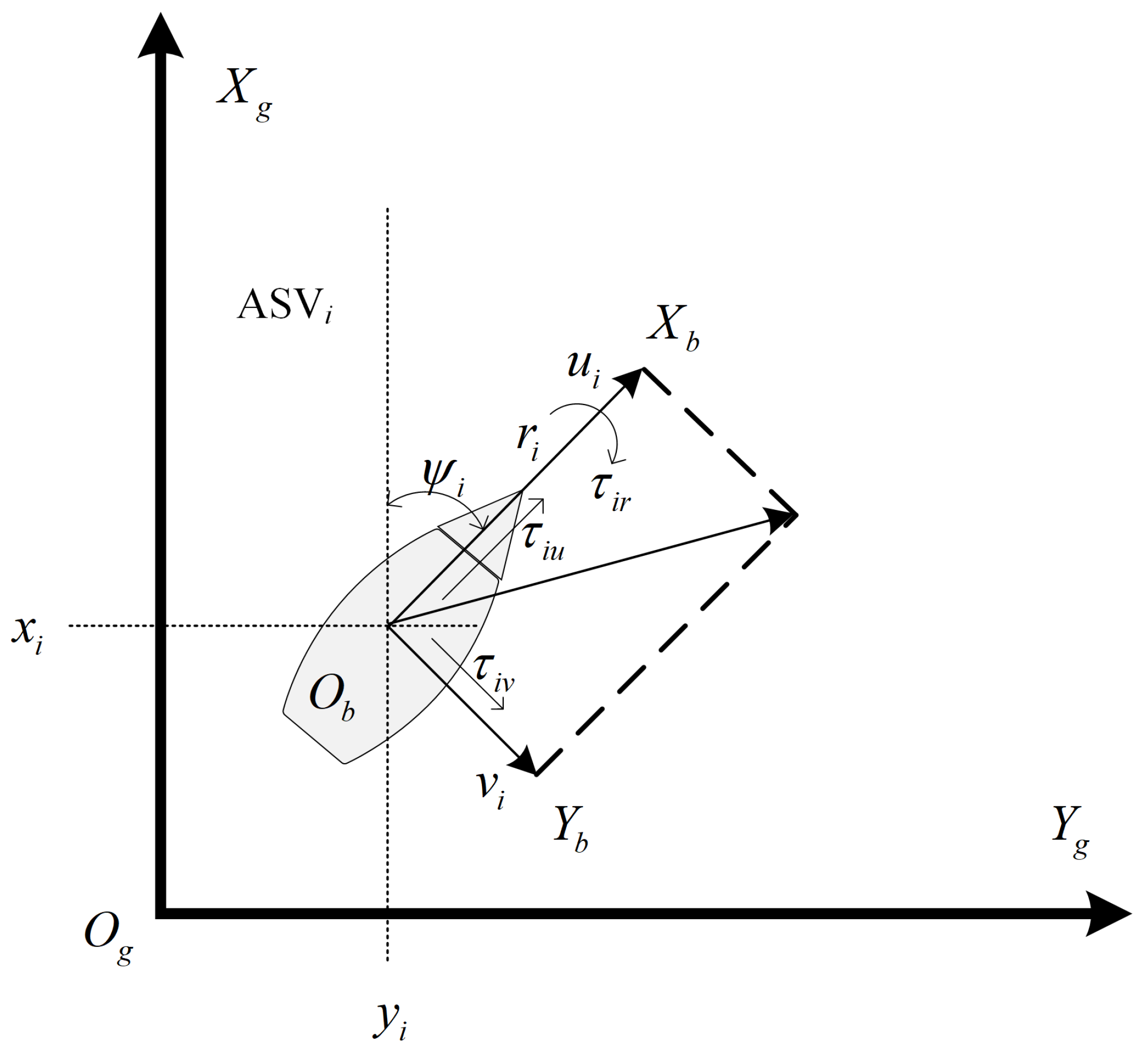
2.1. System Model

Assume a formation of N ASVs, represented by the index set $\mathcal{M}=\left\{1,2,\dots ,N\right\}$, where each vehicle is uniquely labeled with a subscript $i\in \mathcal{M}$. As outlined in [45], the three degrees of freedom model representing the motion of the i-th ASV, formulated using principles of kinematics and rigid body mechanics, can be expressed as follows:

$$\left\{\begin{array}{cc}\hfill {\dot{\mathit{\eta }}}_i& =\mathit{J}\left({\psi }_i\right){\mathit{\upsilon }}_i,\hfill \\ \hfill {\dot{\mathit{\upsilon }}}_i& ={\mathit{M}}_i^{-1}(-{\mathit{C}}_i\left({\mathit{\upsilon }}_i\right){\mathit{\upsilon }}_i-{\mathit{D}}_i\left({\mathit{\upsilon }}_i\right){\mathit{\upsilon }}_i+{\mathit{\tau }}_i+{\mathit{d}}_i)\hfill \end{array}\right.$$

(1)

where the vector ${\mathit{\eta }}_i={\left[\begin{array}{ccc}{x}_i& y_i& {\psi }_i\end{array}\right]}^{\top }\in {\mathbb{R}}^3$ represents the position and yaw angle of the i-th ASV in the inertial coordinate system. ${\mathit{\upsilon }}_i={\left[\begin{array}{ccc}{u}_i& v_i& r_i\end{array}\right]}^{\top }\in {\mathbb{R}}^3$ indicates the velocity of the i-th ASV in the body-fixed frame, including longitudinal, lateral, and rotational components. The rotation matrix $\mathit{J}\left({\psi }_i\right)$ defines the transformation between the body-fixed and inertial frames for the i-th ASV. ${\mathit{M}}_i\in {\mathbb{R}}^{3\times 3}$ is the inertia matrix of the i-th ASV. The matrix ${\mathit{C}}_i\left({\mathit{\upsilon }}_i\right)\in {\mathbb{R}}^{3\times 3}$ accounts for Coriolis and centripetal forces, while matrix ${\mathit{D}}_i\left({\mathit{\upsilon }}_i\right)\in {\mathbb{R}}^{3\times 3}$ represents hydrodynamic damping of the i-th ASV. The control input vector ${\mathit{\tau }}_i={\left[\begin{array}{ccc}{\tau }_{iu}& {\tau }_{iv}& {\tau }_{ir}\end{array}\right]}^{\top }\in {\mathbb{R}}^3$ corresponds to the forces and moments applied to the i-th ASV, and ${\mathit{d}}_i={\left[\begin{array}{ccc}{d}_{iu}& d_{iv}& d_{ir}\end{array}\right]}^{\top }\in {\mathbb{R}}^3$ describes the environmental disturbances acting on it. The aforementioned vectors are illustrated in Figure 1. The aforementioned matrices ${\mathit{M}}_i$, ${\mathit{C}}_i\left({\mathit{\upsilon }}_i\right)$, $\mathit{J}\left({\psi }_i\right)$, and ${\mathit{D}}_i\left({\mathit{\upsilon }}_i\right)$ are given by

$${\mathit{M}}_i=\left[\begin{array}{ccc}{m}_{11i}& 0& 0\\ 0& m_{22i}& m_{23i}\\ 0& m_{32i}& m_{33i}\end{array}\right],\mathit{J}\left({\psi }_i\right)=\left[\begin{array}{ccc}cos\left({\psi }_i\right)& -sin\left({\psi }_i\right)& 0\\ sin\left({\psi }_i\right)& cos\left({\psi }_i\right)& 0\\ 0& 0& 1\end{array}\right],$$

$${\mathit{C}}_i\left({\mathit{\upsilon }}_i\right)=\left[\begin{array}{ccc}0& 0& c_{13i}\\ 0& 0& c_{23i}\\ -c_{13i}& -c_{23i}& 0\end{array}\right],{\mathit{D}}_i\left({\mathit{\upsilon }}_i\right)=\left[\begin{array}{ccc}{d}_{11i}& 0& 0\\ 0& d_{22i}& d_{23i}\\ 0& d_{32i}& d_{33i}\end{array}\right]$$

where each entry in ${\mathit{C}}_i\left({\mathit{\upsilon }}_i\right)$ corresponds to a product of mass/added mass parameters and velocity variables, reflecting the Coriolis and centripetal (centrifugal) force terms arising from the coupling between velocity and inertia parameters. Each entry in ${\mathit{D}}_i\left({\mathit{\upsilon }}_i\right)$ represents the hydrodynamic damping force or moment acting on the vessel in the corresponding degree of freedom.

To describe the communication relationships among ASVs, the formation’s network topologies are modeled as a set of undirected graphs ${\left\{G_k\right\}}_{k=1}^S$, where each graph $G_k=\left(\mathcal{V},{\mathcal{E}}_k\right)$ represents a topology in a known switching sequence. $\mathcal{V}=\{{\nu }_1,\dots ,{\nu }_N\}$ denotes the set of vertices corresponding to the ASVs, and ${\mathcal{E}}_k\subseteq \left\{{\nu }_i,{\nu }_j\mid i,j\in \mathcal{M},i\ne j\right\}$ represents the edge set of $G_k$, with each edge $({\nu }_i,{\nu }_j)$ indicating a bidirectional communication link between the i-th and j-th ASVs. Let ${\mathcal{A}}_k=\left[a_{ij}^{\left(k\right)}\right]\in {\mathbb{R}}^{N\times N}$ be the adjacency matrix of $G_k$, where $a_{ij}^{\left(k\right)}=1$ if $({\nu }_i,{\nu }_j)\in {\mathcal{E}}_k$, and $a_{ij}^{\left(k\right)}=0$ otherwise. The neighbors of the i-th ASV under topology $G_k$ are represented by ${\mathcal{N}}_i^{\left(k\right)}=\{j\mid a_{ij}^{\left(k\right)}=1\}$. The degree matrix for $G_k$ is defined as ${\mathcal{D}}_k=\mathrm{diag}\{b^{\left(k\right)}\left({\nu }_1\right),\dots ,b^{\left(k\right)}\left({\nu }_N\right)\}\in {\mathbb{R}}^{N\times N}$, where $b^{\left(k\right)}\left({\nu }_i\right)={\sum }_{j\in \mathcal{M}}{a}_{ij}^{\left(k\right)}$ denotes the degree of node ${\nu }_i$ in $G_k$. The Laplacian matrix for the k-th topology is given by ${\mathit{L}}_k={\mathcal{D}}_k-{\mathcal{A}}_k$.

Lemma 1

([46]). For a connected undirected graph G with N vertices, let ${\lambda }_i$ represent the i-th eigenvalue of its Laplacian matrix $\mathit{L}$. The eigenvalues are non-negative and satisfy $0\le {\lambda }_i\le N$. Additionally, the eigenvalue 0 has a multiplicity of one, and its corresponding eigenvector is ${\mathbf{1}}_{N\times 1}$.

Lemma 2

([47]). For a general system described as

$$\dot{\mathit{e}}\left(t\right)=\mathit{f}(\mathit{e}\left(t\right),\mathit{u}\left(t\right),\mathit{\omega }\left(t\right))$$

where $\mathit{e}\left(t\right)$ represents the system state to be stabilized, $\mathit{u}\left(t\right)$ is the control input, $\mathit{\omega }\left(t\right)$ denotes the external disturbance, and $\mathit{f}\{·\}$ represents the system dynamics. Then, the $H_{\infty }$ control problem aims to design a control law $\mathit{u}={\mathit{u}}^{\ast }$ such that

1.

The system state $\mathit{e}\left(t\right)$ converges to the origin when $\mathit{\omega }\left(t\right)=\mathbf{0}$;

2.

The following inequality holds for the zero initial state $\mathit{e}\left(0\right)=\mathbf{0}$

$${\int }_0^{+\infty }{∥\mathit{e}\left(t\right)∥}^2\mathrm{d}t\le {\gamma }^2{\int }_0^{+\infty }{∥\mathit{\omega }\left(t\right)∥}^2\mathrm{d}t$$

where $\gamma >0$ is a designed scalar representing the performance bound.

In this paper, aperiodic sampled communication with transmission delay within the formation is considered. Specifically, the sampling instants are denoted as $t_l$, where $l\in {\mathbb{N}}^{+}$ and $t_1=0$. The l-th sampling period is defined by $T_l=t_{l+1}-t_l$, with $0<T_l\le T_m$, where $T_m$ represents the maximum allowable sampling interval. The communication time delay within the formation, denoted by $T_d$, is assumed to be constant throughout. Figure 2 illustrates the data communication process between two ASVs, where the sampling communication period and transmission delay are indicated in the figure. For the 1-th ASV, it can access the ${\mathrm{data}}_2\left(t_3\right)$ from the 2-nd ASV only after $t_3+T_d$, and new data will be received again after $t_4+T_d$, as shown by the green area in the figure.

Remark 1.

As highlighted in prior studies [48,49], aperiodic sampled-data systems provide a more realistic framework for modeling and analyzing networked control systems, especially in complex environments such as the marine domain. To facilitate the theoretical analysis of leaderless formation control under non-ideal communication conditions, the formation controller in this paper is designed based on the assumptions of fixed transmission delay and accurate state information. In real-world multi-ASV systems, communication delays may be time varying, state measurements can be affected by noise and inaccuracies, and packet loss may occur. Future work will extend the proposed approach to address these practical challenges.

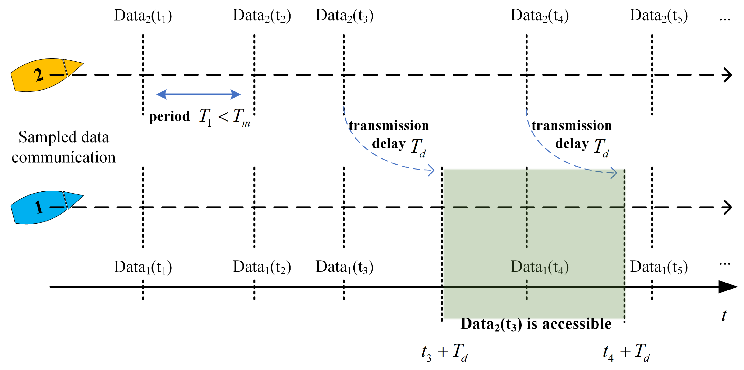
2.2. Problem Statement

To describe the desired locations of the ASVs in the leaderless frame, we introduce the concept of the IFC, which acts as a virtual reference center for the formation and facilitates the description of the group motion. The vectors ${\mathit{\alpha }}_i\in {\mathbb{R}}^3$, $i\in \mathcal{M}$ are defined to represent the desired displacements of each ASV relative to the IFC.

Definition 1.

The multi-ASV system is considered to achieve leaderless formation if a control input ${\mathit{\tau }}_{\mathbf{I}}$ can be designed in Equation (1) such that

$$\underset{t\to +\infty }{lim}∥{\mathit{\eta }}_i-{\mathit{\alpha }}_i-\left({\mathit{\eta }}_j-{\mathit{\alpha }}_j\right)∥=0$$

(2)

Then, let ${\mathit{\varsigma }}_i={\left[\begin{array}{ccc}{\varsigma }_{ix}& {\varsigma }_{iy}& {\varsigma }_{i\psi }\end{array}\right]}^{\top }={\mathit{\eta }}_i-{\mathit{\alpha }}_i$ and ${\mathit{ϵ}}_i=\mathit{J}\left({\psi }_i\right){\mathit{\upsilon }}_i$, where $i\in \mathcal{M}$. It follows that $\dot{{\mathit{\varsigma }}_i}=\dot{{\mathit{\eta }}_i}-\dot{{\mathit{\alpha }}_i}={\mathit{ϵ}}_i$. Furthermore, Definition 1 can be reformulated as ${lim}_{t\to +\infty }∥{\mathit{\varsigma }}_i-{\mathit{o}}_p∥=0$, where ${\mathit{o}}_p\in {\mathbb{R}}^3$ represents the position of the IFC.

For clarity of notation, the invertible matrix is defined as ${\mathrm{\Gamma }}_i=\mathit{J}\left({\psi }_i\right){\mathit{M}}_i^{-1}\in {\mathbb{R}}^{3\times 3}$. The terms ${\mathit{C}}_i$ and ${\mathit{D}}_i$ are shorthand for ${\mathit{C}}_i\left({\mathit{\upsilon }}_i\right)$ and ${\mathit{D}}_i\left({\mathit{\upsilon }}_i\right)$, respectively. Define ${\mathit{\tau }}_i^{\prime }={\mathrm{\Gamma }}_i{\mathit{\tau }}_i$ as the virtual controller and ${\mathit{d}}_i^{\prime }={\mathrm{\Gamma }}_i{\mathit{d}}_i$. Then, the dynamics of ${\mathit{ϵ}}_i$ are as follows:

$$\begin{array}{cc}\hfill \dot{{\mathit{ϵ}}_i}& =\dot{\mathit{J}}\left({\psi }_i\right){\mathit{\upsilon }}_i+\mathit{J}\left({\psi }_i\right)\dot{{\mathit{\upsilon }}_i}\hfill \\ \hfill & =\mathit{J}\left({\psi }_i\right){\mathit{R}}_i{\mathit{\upsilon }}_i+{\mathrm{\Gamma }}_i(-{\mathit{C}}_i{\mathit{\upsilon }}_i-{\mathit{D}}_i{\mathit{\upsilon }}_i+{\mathit{\tau }}_i+{\mathit{d}}_i)\hfill \\ \hfill & ={\mathit{R}}_i{\mathit{\xi }}_i-{\mathrm{\Gamma }}_i\left({\mathit{C}}_i+{\mathit{D}}_i\right){\mathit{\upsilon }}_i+{\mathit{\tau }}_i^{\prime }+{\mathit{d}}_i^{\prime }\hfill \end{array}$$

(3)

where

$${\mathit{R}}_i=\left[\begin{array}{ccc}0& -r_i& 0\\ r_i& 0& 0\\ 0& 0& 0\end{array}\right]\in {\mathbb{R}}^{3\times 3}$$

Let ${\mathit{\zeta }}_i\left(t\right)={\left[\begin{array}{cc}{\mathit{\varsigma }}_i^{\top }& {\mathit{ϵ}}_i^{\top }\end{array}\right]}^{\top }$ represent the integrated state. Further, the dynamics of ${\mathit{\zeta }}_i$ can be derived as follows:

$$\dot{{\mathit{\zeta }}_i}\left(t\right)=\mathit{A}{\mathit{\zeta }}_i\left(t\right)+\mathit{B}\left({\mathit{R}}_i{\mathit{ϵ}}_i-{\mathrm{\Gamma }}_i({\mathit{C}}_i+{\mathit{D}}_i){\mathit{\upsilon }}_i+{\mathit{\tau }}_i^{\prime }+{\mathit{d}}_i^{\prime }\right)$$

(4)

where

$$\mathit{A}=\left[\begin{array}{cc}{\mathbf{0}}_{3\times 3}& {\mathbf{I}}_3\\ {\mathbf{0}}_{3\times 3}& {\mathbf{0}}_{3\times 3}\end{array}\right],\mathit{B}=\left[\begin{array}{c}{\mathbf{0}}_{3\times 3}\\ {\mathbf{I}}_3\end{array}\right]$$

Considering that the ASVs should remain relatively stationary with respect to each other during the formation process, the leaderless formation can also be defined in the following form:

Definition 2.

The multi-ASV system is considered to achieve leaderless formation if a control input ${\mathit{\tau }}_{\mathbf{I}}$ can be designed in Equation (1) such that

$$\underset{t\to +\infty }{lim}∥{\mathit{\zeta }}_i\left(t\right)-{\mathit{\zeta }}_j\left(t\right)∥=0$$

(5)

Similarly, Definition 2 can be extended as ${lim}_{t\to +\infty }\parallel {\mathit{\zeta }}_i\left(t\right)-{\mathit{o}}_f\left(t\right)\parallel =0$, where ${\mathit{o}}_f={\left[\begin{array}{cc}{\mathit{o}}_p^{\top }& {\mathit{o}}_v^{\top }\end{array}\right]}^{\top }\in {\mathbb{R}}^6$ represents the integrated state of the position and velocity of the IFC.

Lemma 3

([50]). For matrices $\mathit{P}$, $\mathit{Q}$, and $\mathit{A}$ of appropriate dimensions, the following inequalities hold:

$$\begin{array}{cc}\hfill & {\mathit{P}}^{\top }\mathit{Q}+{\mathit{Q}}^{\top }\mathit{P}\le {\mu }_1{\mathit{P}}^{\top }\mathit{P}+{\mu }_1^{-1}{\mathit{Q}}^{\top }\mathit{Q},\hfill \end{array}$$

(6)

$$\begin{array}{cc}\hfill & {\mathit{P}}^{\top }\mathit{A}\mathit{Q}+{\mathit{Q}}^{\top }\mathit{A}\mathit{P}\le {\mu }_2^{-1}{\mathit{P}}^{\top }\mathit{P}+{\mu }_2{\mu }_3{\mathit{Q}}^{\top }\mathit{Q}\hfill \end{array}$$

(7)

where ${\mu }_1,{\mu }_2>0$, and ${\mu }_3$ satisfies ${\mathit{A}}^{\top }\mathit{A}\le {\mu }_3\mathbf{I}$.

Lemma 4

([51]). Let $\mathit{A}\in {\mathbb{R}}^{n\times n}$ be a constant positive definite matrix. For a continuously differentiable vector function $\mathit{f}:[a_1,a_2]\to {\mathbb{R}}^n$, the following inequality holds:

$$(b-a){\int }_a^b{\mathit{f}}^{\top }\left(t\right)\mathit{A}\mathit{f}\left(t\right)\mathrm{d}t\ge {\left({\int }_a^b\mathit{f}\left(t\right)\mathrm{d}t\right)}^{\top }\mathit{A}\left({\int }_a^b\mathit{f}\left(t\right)\mathrm{d}t\right)$$

(8)

Lemma 5

([52]). For a continuously differentiable function $\mathit{f}:[a_1,a_2]\to {\mathbb{R}}^n$, define ${\mathit{h}}_1=\mathit{f}\left(a_2\right)-\mathit{f}\left(a_1\right)$ and ${\mathit{h}}_2=\mathit{f}\left(a_2\right)+\mathit{f}\left(a_1\right)-\left(2/(a_2-a_1)\right){\int }_{a_1}^{a_2}\mathit{f}\left(\alpha \right)\mathrm{d}\alpha$. The following inequality holds:

$${\int }_{a_1}^{a_2}{\dot{\mathit{f}}}^{\top }\left(\alpha \right)\mathit{A}\dot{\mathit{f}}\left(\alpha \right)\mathrm{d}\alpha \ge {\displaystyle \frac{1}{a_2-a_1}}{\mathit{h}}_1^{\top }\mathit{A}{\mathit{h}}_1+{\displaystyle \frac{3}{a_2-a_1}}{\mathit{h}}_2^{\top }\mathit{A}{\mathit{h}}_2$$

(9)

where $\mathit{A}\in {\mathbb{R}}^{n\times n}$ is a positive definite matrix.

Lemma 6

([53]). Define ${\mathit{f}}_1,{\mathit{f}}_2,\dots ,{\mathit{f}}_N:{\mathbb{R}}^m\to \mathbb{R}$ as a set of functions positive on the open subset $\Lambda \subseteq {\mathbb{R}}^m$. Then, for a set of scalars $\{a_i\mid a_i>0,{\sum }_{i=1}^N{a}_i=1\}$, the following equality holds:

$$min\sum _{i=1}^N{\displaystyle \frac{1}{a_i}}{\mathit{f}}_i\left(\mathit{x}\right)=\sum _{i=1}^N{\mathit{f}}_i\left(\mathit{x}\right)+\underset{{\mathit{g}}_{i,j}\left(t\right)}{max}\sum _{i\ne j}^N{\mathit{g}}_{i,j}\left(\mathit{x}\right),\mathit{x}\in \Lambda$$

(10)

subject to

$$\left\{{\mathit{g}}_{i,j}:{\mathbb{R}}^m\to \mathbb{R},{\mathit{g}}_{i,j}\left(\mathit{x}\right)={\mathit{g}}_{j,i}\left(\mathit{x}\right),\left[\begin{array}{cc}{\mathit{f}}_i\left(\mathit{x}\right)& {\mathit{g}}_{i,j}\left(\mathit{x}\right)\\ {\mathit{g}}_{i,j}\left(\mathit{x}\right)& {\mathit{f}}_j\left(\mathit{x}\right)\end{array}\right]\ge \mathbf{0}\right\}$$

To facilitate a better understanding of the subsequent controller design and theoretical analysis, a flowchart is provided in Figure 3. This flowchart outlines the logical sequence and interconnections of the main equations and steps in the proposed methodology.

3. Controller Design and Stability Analysis

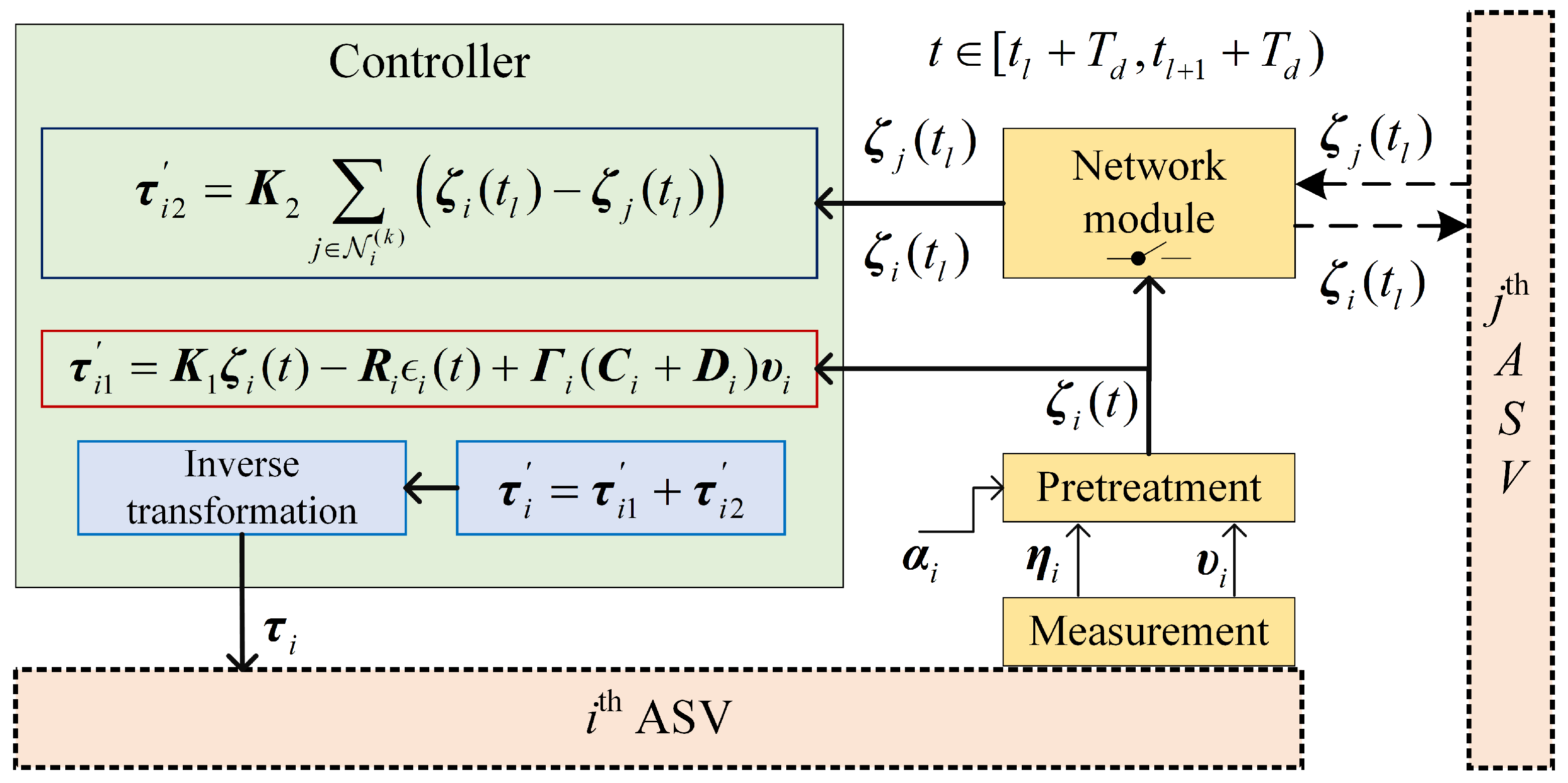
3.1. Controller Design

According to the description of the communication model mentioned above, the i-th ASV can acquire the data from j-th ASV where $j\in {\mathcal{N}}_i$ at the sampling instant $t_l$ within the time interval $[t_l+T_d,t_{l+1}+T_d)$. Thus, the designed controller ${\mathit{\tau }}_i^{\prime }$ takes the following form:

$${\mathit{\tau }}_i^{\prime }={\mathit{K}}_1{\mathit{\zeta }}_i\left(t\right)-{\mathit{R}}_i{\mathit{ϵ}}_i\left(t\right)+{\mathrm{\Gamma }}_i({\mathit{C}}_i+{\mathit{D}}_i){\mathit{\upsilon }}_i+{\mathit{K}}_2\sum _{j\in {\mathcal{N}}_i^{\left(k\right)}}\left({\mathit{\zeta }}_i\left(t_l\right)-{\mathit{\zeta }}_j\left(t_l\right)\right)$$

(11)

where $t\in \left[t_k+T_d,t_{k+1}+T_d\right)$, with ${\mathit{K}}_1$, ${\mathit{K}}_2\in {\mathbb{R}}^{3\times 6}$ being feedforward and consensus gain matrices separately.

By substituting Equation (11) to Equation (4), we obtain the following result:

$$\dot{{\mathit{\zeta }}_i}\left(t\right)=(\mathit{A}+{\mathit{BK}}_1){\mathit{\zeta }}_i\left(t\right)+\mathit{B}{\mathit{K}}_2\sum _{j\in {\mathcal{N}}_i^{\left(k\right)}}({\mathit{\zeta }}_i\left(t_l\right)-{\mathit{\zeta }}_j\left(t_l\right))+\mathit{B}{\mathit{d}}_i^{\prime }\left(t\right)$$

(12)

To investigate the state evolution of all formation members, the compact forms ${\mathit{\zeta }}_c={\left[\begin{array}{ccc}{\mathit{\zeta }}_1^{\top }& \dots & {\mathit{\zeta }}_N^{\top }\end{array}\right]}^{\top }$ and ${\mathit{d}}_c={\left[\begin{array}{ccc}{\mathit{d}}_1^{\top }& \dots & {\mathit{d}}_N^{\top }\end{array}\right]}^{\top }$ are defined. According to Equation (12), the dynamics of ${\mathit{\zeta }}_c$ can be derived as follows:

$${\dot{\mathit{\zeta }}}_c\left(t\right)=\left({\mathbf{I}}_N\otimes (\mathit{A}+{\mathit{BK}}_1)\right){\mathit{\zeta }}_c\left(t\right)+\left({\mathit{L}}_k\otimes \left({\mathit{BK}}_2\right)\right){\mathit{\zeta }}_c\left(t_l\right)+({\mathbf{I}}_N\otimes \mathit{B}){\mathit{d}}_c^{\prime }\left(t\right)$$

(13)

Note that $t_l+T_d\le t<t_{l+1}+T_d$ and $0<t_{l+1}-t_l\le T_m$. By defining $h_l\left(t\right)=t-t_l$, Equation (13) can be reformulated as follows:

$${\dot{\mathit{\zeta }}}_c\left(t\right)=\left({\mathbf{I}}_N\otimes (\mathit{A}+{\mathit{BK}}_1)\right){\mathit{\zeta }}_c\left(t\right)+\left({\mathit{L}}_k\otimes \left({\mathit{BK}}_2\right)\right){\mathit{\zeta }}_c(t-h_l\left(t\right))+({\mathbf{I}}_N\otimes \mathit{B}){\mathit{d}}_c^{\prime }\left(t\right)$$

(14)

where $T_d\le h_l\left(t\right)<T_m+T_d$.

Since ${\mathit{L}}_k$ is a real symmetric matrix, Lemma 1 guarantees the existence of a normalized orthogonal matrix ${\mathit{D}}_k$ such that the following equations holds:

$${\mathit{D}}_k^{\top }{\mathit{L}}_k{\mathit{D}}_k={\mathbf{\Pi }}_k=\left[\begin{array}{cc}{\lambda }_1^{\left(k\right)}& {\mathbf{0}}_{N-1\times N-1}\\ & {\mathbf{\Pi }}_k^{\ast }\end{array}\right]\in {\mathbb{R}}^{N\times N}$$

(15)

where

$${\mathbf{\Pi }}_k^{\ast }=\left[\begin{array}{ccc}{\lambda }_2^{\left(k\right)}& \dots & 0\\ ⋮& \ddots & ⋮\\ & \dots & {\lambda }_N^{\left(k\right)}\end{array}\right]\in {\mathbb{R}}^{(N-1)\times (N-1)},{\mathit{D}}_k=\left[\begin{array}{cc}{\displaystyle \frac{{\mathbf{1}}_{N\times 1}}{\sqrt{N}}}& {\mathit{D}}_k^{\ast }\end{array}\right]\in {\mathbb{R}}^{N\times N}$$

In Equation (15), the first eigenvalue ${\lambda }_1^{\left(k\right)}=0$, while the remaining eigenvalues ${\lambda }_2^{\left(k\right)},{\lambda }_3^{\left(k\right)},\dots ,{\lambda }_N^{\left(k\right)}$ are arranged in ascending order within the matrix ${\mathbf{\Pi }}_k^{\ast }$. The matrix ${\mathit{D}}_k^{\ast }\in {\mathbb{R}}^{N\times (N-1)}$ consists of the remaining normalized eigenvectors. Across all topologies, the largest eigenvalue is represented by ${\lambda }_m$.

To facilitate subsequent analysis, the state variables ${\mathit{z}}_c\left(t\right)\in {\mathbb{R}}^{6N}$ and ${\mathit{w}}_c\left(t\right)\in {\mathbb{R}}^{3N}$ are introduced through the following state-space transformations:

$${\mathit{z}}_c\left(t\right)=\left({\mathit{D}}_k^{\top }\otimes {\mathbf{I}}_6\right){\mathit{\zeta }}_c\left(t\right)=\left[\begin{array}{c}{\mathit{z}}_1\left(t\right)\\ ⋮\\ {\mathit{z}}_N\left(t\right)\end{array}\right]=\left[\begin{array}{c}{\overline{\mathit{z}}}_1\left(t\right)\\ {\overline{\mathit{z}}}_2\left(t\right)\end{array}\right],$$

(16)

$${\mathit{w}}_c\left(t\right)=\left({\mathit{D}}_k^{\top }\otimes {\mathbf{I}}_3\right){\mathit{d}}_c^{\prime }\left(t\right)=\left[\begin{array}{c}{\mathit{w}}_1\left(t\right)\\ ⋮\\ {\mathit{w}}_N\left(t\right)\end{array}\right]=\left[\begin{array}{c}{\overline{\mathit{w}}}_1\left(t\right)\\ {\overline{\mathit{w}}}_2\left(t\right)\end{array}\right]$$

(17)

where ${\overline{\mathit{z}}}_1\left(t\right)={\mathit{z}}_1\left(t\right)\in {\mathbb{R}}^6$, and ${\overline{\mathit{w}}}_1\left(t\right)={\mathit{w}}_1\left(t\right)\in {\mathbb{R}}^3$. Based on Equations (14), (16) and (17), the dynamics of ${\mathit{z}}_c\left(t\right)$ can be deduced as follows:

$$\dot{{\mathit{z}}_c}\left(t\right)=\left({\mathbf{I}}_N\otimes (\mathit{A}+{\mathit{BK}}_1)\right){\mathit{z}}_c\left(t\right)+\left({\mathbf{\Pi }}_k\otimes {\mathit{BK}}_2\right){\mathit{z}}_c(t-h_l\left(t\right))+({\mathbf{I}}_N\otimes \mathit{B}){\mathit{w}}_c\left(t\right)$$

(18)

Subsequently, from Equation (18), the dynamics of ${\overline{\mathit{z}}}_1\left(t\right)$ and ${\overline{\mathit{z}}}_2\left(t\right)$ can be derived as follows:

$$\begin{array}{cc}\hfill & {\dot{\overline{\mathit{z}}}}_1\left(t\right)=(\mathit{A}+{\mathit{BK}}_1){\overline{\mathit{z}}}_1\left(t\right)+\mathit{B}{\overline{\mathit{w}}}_1\left(t\right),\hfill \end{array}$$

(19)

$$\begin{array}{cc}\hfill & {\dot{\overline{\mathit{z}}}}_2\left(t\right)=\left({\mathbf{I}}_{N-1}\otimes (\mathit{A}+{\mathit{BK}}_1)\right){\overline{\mathit{z}}}_2\left(t\right)+\left({\mathbf{\Pi }}_k^{\ast }\otimes {\mathit{BK}}_2\right){\overline{\mathit{z}}}_2(t-h_l\left(t\right))+\left({\mathbf{I}}_{N-1}\otimes \mathit{B}\right){\overline{\mathit{w}}}_2\left(t\right)\hfill \end{array}$$

(20)

To further analyze the relationship between the original system ${\mathit{\zeta }}_c\left(t\right)$ and translated subsystems ${\overline{\mathit{z}}}_1$ and ${\overline{\mathit{z}}}_2$, we perform the inverse transformation based on Equation (16) as follows:

$$\begin{array}{c}\hfill {\mathit{\zeta }}_c\left(t\right)=\left({\mathit{D}}_k\otimes {\mathbf{I}}_6\right){\mathit{z}}_c\left(t\right)=\left({\displaystyle \frac{{\mathbf{1}}_{N\times 1}}{\sqrt{N}}}\otimes {\mathbf{I}}_6\right){\overline{\mathit{z}}}_1\left(t\right)+\left({\mathit{D}}_k^{\ast }\otimes {\mathbf{I}}_6\right){\overline{\mathit{z}}}_2\left(t\right)\end{array}$$

(21)

According to Equation (21), it can be observed that if the subsystem ${\overline{\mathit{z}}}_2$ can be stabilized such that ${lim}_{t\to +\infty }{\overline{\mathit{z}}}_2\left(t\right)=\mathbf{0}$, then the evolution of ${\mathit{\zeta }}_c\left(t\right)$ is solely influenced by the subsystem ${\overline{\mathit{z}}}_1\left(t\right)$ in Equation (19).

Remark 2.

Note that due to the specific structure of the matrix $({\mathbf{1}}_{N\times 1}/\sqrt{N})\otimes {\mathbf{I}}_6$, when ${\overline{\mathit{z}}}_2$ is stabilized, it can be deduced that ${lim}_{t\to +\infty }{\mathit{\zeta }}_i\left(t\right)={\mathit{\zeta }}_j\left(t\right)$ with $i,j\in \mathcal{M}$, satisfying Definition 2. This indicates an equivalence in stability between ${\overline{\mathit{z}}}_2$ and the leaderless formation. Following a straightforward deduction, the evolution of the IFC can be determined, which will be elaborated in the subsequent text.

Definition 3.

The multi-ASV system is considered to achieve leaderless formation with $H_{\infty }$ performance, if the subsystem ${\overline{\mathit{z}}}_2$ is stabilized with $H_{\infty }$ performance.

To provide a clearer illustration of the operational process of controller Equation (11) within the formation system, a system block diagram is presented in Figure 4. For clarity of exposition, it is assumed in this figure that the data sampled by the j-th ASV at the sampling instant $t_l$ have been received by the i-th ASV after a transmission delay $T_d$, and that the next sampling instant has not yet been triggered at this moment.

3.2. Stability Analysis

In this subsection, based on the controller form designed in Equation (11), several theorems and analyses are presented as follows:

Theorem 1.

Given the network parameters $T_m$, $T_d$, and the predefined feedforward gain ${\mathit{K}}_1\in {\mathbb{R}}^{3\times 6}$, assume there exist a scalar $\delta >0$, matrices $\mathit{P}\in {\mathbb{R}}^{6\times 6}>0$, ${\mathit{Q}}_i\in {\mathbb{R}}^{6\times 6}>0$ for $i=1,\dots ,6$, $\mathit{U}\in {\mathbb{R}}^{6\times 6}$, $\mathbf{\Phi }\in {\mathbb{R}}^{6\times 6}$, and consensus gain ${\mathit{K}}_2\in {\mathbb{R}}^{3\times 6}$, such that the following linear matrix inequalities (LMIs) are satisfied:

$$\begin{array}{cc}\hfill & \left[\begin{array}{ccc}{\mathbf{\Omega }}_a& {\mathit{W}}_5^{\top }\mathbf{\Phi }& {\mathit{W}}_4^{\top }{\mathit{K}}_2^{\top }{\mathit{B}}^{\top }\\ & -\delta {\mathbf{I}}_6& {\mathbf{0}}_{6\times 6}\\ & \ast & -{\delta }^{-1}{\lambda }_m^{-2}{\mathbf{I}}_6\end{array}\right]<0,\hfill \end{array}$$

(22)

$$\begin{array}{cc}\hfill & \left[\begin{array}{cc}{\mathit{Q}}_6& \mathit{U}\\ & {\mathit{Q}}_6\end{array}\right]>0\hfill \end{array}$$

(23)

where ${\mathit{W}}_i=\left[\begin{array}{ccc}{\mathbf{0}}_{6\times 6(i-1)}& {\mathbf{I}}_6& {\mathbf{0}}_{6\times 6(7-i)}\end{array}\right]\in {\mathbb{R}}^{6\times 42}$ for $i=1,\dots ,7$, and ${\mathbf{\Omega }}_a={\sum }_{j=1}^8{\mathbf{\Omega }}_j$ with

$$\begin{array}{cc}\hfill & {\mathbf{\Omega }}_1={\mathit{W}}_5^{\top }\mathit{P}{\mathit{W}}_1+{\mathit{W}}_1^{\top }\mathit{P}{\mathit{W}}_5\hfill \\ \hfill & {\mathbf{\Omega }}_2={\mathit{W}}_2^{\top }({\mathit{Q}}_1-{\mathit{Q}}_2){\mathit{W}}_2+{\mathit{W}}_1^{\top }{\mathit{Q}}_2{\mathit{W}}_1-{\mathit{W}}_3^{\top }{\mathit{Q}}_1{\mathit{W}}_3\hfill \\ \hfill & {\mathbf{\Omega }}_3={\mathit{W}}_1^{\top }(T_d{\mathit{Q}}_3+T_m{\mathit{Q}}_4){\mathit{W}}_1\hfill \\ \hfill & {\mathbf{\Omega }}_4=-{\mathit{W}}_6^{\top }{\displaystyle \frac{{\mathit{Q}}_3}{T_d}}{\mathit{W}}_6-{\mathit{W}}_7^{\top }{\displaystyle \frac{{\mathit{Q}}_4}{T_m}}{\mathit{W}}_7\hfill \\ \hfill & {\mathbf{\Omega }}_5={\mathit{W}}_5^{\top }(T_d{\mathit{Q}}_5+T_m{\mathit{Q}}_6){\mathit{W}}_5\hfill \\ \hfill & {\mathbf{\Omega }}_6=-{({\mathit{W}}_1-{\mathit{W}}_2)}^{\top }{\displaystyle \frac{{\mathit{Q}}_5}{T_d}}({\mathit{W}}_1-{\mathit{W}}_2)-{({\mathit{W}}_1+{\mathit{W}}_2-{\displaystyle \frac{2{\mathit{W}}_6}{T_d}})}^{\top }{\displaystyle \frac{3{\mathit{Q}}_5}{T_d}}({\mathit{W}}_1+{\mathit{W}}_2-{\displaystyle \frac{2{\mathit{W}}_6}{T_d}})\hfill \\ \hfill & {\mathbf{\Omega }}_7=T_m^{-1}{\left[\begin{array}{c}{\mathit{W}}_2\\ {\mathit{W}}_4\\ {\mathit{W}}_3\end{array}\right]}^{\top }\left[\begin{array}{ccc}-{\mathit{Q}}_6& {\mathit{Q}}_6^{\top }-{\mathit{U}}^{\top }& \mathit{U}\\ \ast & -2{\mathit{Q}}_6+\mathit{U}+{\mathit{U}}^{\top }& {\mathit{Q}}_6^{\top }-\mathit{U}\\ \ast & \ast & -{\mathit{Q}}_6\end{array}\right]\left[\begin{array}{c}{\mathit{W}}_2\\ {\mathit{W}}_4\\ {\mathit{W}}_3\end{array}\right]\hfill \\ \hfill & {\mathbf{\Omega }}_8={\mathit{W}}_5^{\top }(-\mathbf{\Phi }-{\mathbf{\Phi }}^{\top }){\mathit{W}}_5+{\mathit{W}}_5^{\top }\left(\mathbf{\Phi }(\mathit{A}+{\mathit{BK}}_1)\right){\mathit{W}}_1+{\mathit{W}}_1^{\top }{\left(\mathbf{\Phi }(\mathit{A}+{\mathit{BK}}_1)\right)}^{\top }{\mathit{W}}_5\hfill \end{array}$$

Then, given any initial state and with ${\overline{\mathit{w}}}_2\left(t\right)=\mathbf{0}$, the proposed controller in Equation (11) guarantees that the subsystem ${\overline{\mathit{z}}}_2\left(t\right)$ achieves asymptotic stability.

Proof of Theorem 1 

Note that the subsystem ${\overline{\mathit{z}}}_2\left(t\right)$ in Equation (20) is a time-delay system, the following Lyapunov–Krasovskii functional (LKF) is employed:

$$V\left(t\right)=\sum _{i=1}^4{V}_i\left(t\right)$$

(24)

where

$$\begin{array}{cc}\hfill & V_1\left(t\right)={\overline{\mathit{z}}}_2^{\top }\left(t\right)({\mathbf{I}}_{N-1}\otimes \mathit{P}){\overline{\mathit{z}}}_2\left(t\right)\hfill \\ \hfill & V_2\left(t\right)={\int }_{t-T_d-T_m}^{t-T_d}{\overline{\mathit{z}}}_2^{\top }\left(\alpha \right)({\mathbf{I}}_{N-1}\otimes {\mathit{Q}}_1){\overline{\mathit{z}}}_2\left(\alpha \right)\mathrm{d}\alpha +{\int }_{t-T_d}^t{\overline{\mathit{z}}}_2^{\top }\left(\alpha \right)({\mathbf{I}}_{N-1}\otimes {\mathit{Q}}_2){\overline{\mathit{z}}}_2\left(\alpha \right)\mathrm{d}\alpha \hfill \\ \hfill & V_3\left(t\right)={\int }_{-T_d}^0{\int }_{t+\beta }^t{\overline{\mathit{z}}}_2^{\top }\left(\alpha \right)({\mathbf{I}}_{N-1}\otimes {\mathit{Q}}_3){\overline{\mathit{z}}}_2\left(\alpha \right)\mathrm{d}\alpha \mathrm{d}\beta +{\int }_{-T_m-T_d}^{-T_d}{\int }_{t+\beta }^t{\overline{\mathit{z}}}_2^{\top }\left(\alpha \right)({\mathbf{I}}_{N-1}\otimes {\mathit{Q}}_4){\overline{\mathit{z}}}_2\left(\alpha \right)\mathrm{d}\alpha \mathrm{d}\beta \hfill \\ \hfill & V_4\left(t\right)={\int }_{-T_d}^0{\int }_{t+\beta }^t{\dot{\overline{\mathit{z}}}}_2^{\top }\left(\alpha \right)({\mathbf{I}}_{N-1}\otimes {\mathit{Q}}_5){\dot{\overline{\mathit{z}}}}_2\left(\alpha \right)\mathrm{d}\alpha \mathrm{d}\beta +{\int }_{-T_m-T_d}^{-T_d}{\int }_{t+\beta }^t{\dot{\overline{\mathit{z}}}}_2^{\top }\left(\alpha \right)({\mathbf{I}}_{N-1}\otimes {\mathit{Q}}_6){\dot{\overline{\mathit{z}}}}_2\left(\alpha \right)\mathrm{d}\alpha \mathrm{d}\beta \hfill \end{array}$$

To streamline the representation of variables during the derivation, we define the integrated vector ${\mathit{x}}_i\in {\mathbb{R}}^{42}$ for $i=2,\dots ,N$ as follows:

$$\begin{array}{cc}\hfill {\mathit{x}}_i\left(t\right)=[& {\mathit{z}}_i^{\top }\left(t\right){\mathit{z}}_i^{\top }(t-T_d){\mathit{z}}_i^{\top }(t-T_d-T_m){\mathit{z}}_i^{\top }(t-h_l\left(t\right)){\dot{\mathit{z}}}_i^{\top }\left(t\right)\hfill \end{array}$$

(25)

$$\begin{array}{cc}& {\int }_{t-T_d}^t{\mathit{z}}_i^{\top }\left(\alpha \right)\mathrm{d}\alpha {\int }_{t-T_d-T_m}^{t-T_d}{\mathit{z}}_i^{\top }\left(\alpha \right)\mathrm{d}\alpha {]}^{\top }\hfill \end{array}$$

(26)

Then, the derivative of the LKF, denoted as $\dot{V}\left(t\right)={\sum }_{i=1}^4\dot{V_i}\left(t\right)$, can be derived as follows:

$$\begin{array}{c}\hfill \begin{array}{cc}\hfill {\dot{V}}_1\left(t\right)=& {\dot{\overline{\mathit{z}}}}_2^{\top }\left(t\right)({\mathbf{I}}_{N-1}\otimes \mathit{P}){\overline{\mathit{z}}}_2\left(t\right)+{\overline{\mathit{z}}}_2^{\top }\left(t\right)({\mathbf{I}}_{N-1}\otimes \mathit{P}){\dot{\overline{\mathit{z}}}}_2^{\top }\left(t\right)\hfill \\ \hfill =& \sum _{i=2}^N\left\{{\dot{\mathit{z}}}_i^{\top }\left(t\right)\mathit{P}{\mathit{z}}_i\left(t\right)+{\mathit{z}}_i^{\top }\left(t\right)\mathit{P}{\dot{\mathit{z}}}_i\left(t\right)\right\}\hfill \\ \hfill =& \sum _{i=2}^N{\mathit{x}}_i^{\top }\left(t\right){\mathbf{\Omega }}_1{\mathit{x}}_i\left(t\right)\hfill \end{array}\end{array}$$

(27)

$$\begin{array}{cc}\hfill {\dot{V}}_2\left(t\right)=& {\overline{\mathit{z}}}_2^{\top }(t-T_d)({\mathbf{I}}_{N-1}\otimes {\mathit{Q}}_1){\overline{\mathit{z}}}_2(t-T_d)-{\overline{\mathit{z}}}_2^{\top }(t-T_d)({\mathbf{I}}_{N-1}\otimes {\mathit{Q}}_2){\overline{\mathit{z}}}_2(t-T_d)\hfill \\ & +{\overline{\mathit{z}}}_2^{\top }\left(t\right)({\mathbf{I}}_{N-1}\otimes {\mathit{Q}}_2){\overline{\mathit{z}}}_2\left(t\right)-{\overline{\mathit{z}}}_2^{\top }(t-T_d-T_m)({\mathbf{I}}_{N-1}\otimes {\mathit{Q}}_1){\overline{\mathit{z}}}_2(t-T_d-T_m)\hfill \\ \hfill =& \sum _{i=2}^N\{{\mathit{z}}_i^{\top }(t-T_d){\mathit{Q}}_1{\mathit{z}}_i(t-T_d)-{\mathit{z}}_i^{\top }(t-T_d){\mathit{Q}}_2{\mathit{z}}_i(t-T_d)\hfill \\ & +{\mathit{z}}_i^{\top }\left(t\right){\mathit{Q}}_2{\mathit{z}}_i\left(t\right)-{\mathit{z}}_i^{\top }(t-T_d-T_m){\mathit{Q}}_1{\mathit{z}}_i(t-T_d-T_m)\}\hfill \\ \hfill =& \sum _{i=2}^N{\mathit{x}}_i^{\top }\left(t\right){\mathbf{\Omega }}_2{\mathit{x}}_i\left(t\right)\hfill \end{array}$$

(28)

$$\begin{array}{cc}\hfill {\dot{V}}_3\left(t\right)=& T_d{\overline{\mathit{z}}}_2^{\top }\left(t\right)({\mathbf{I}}_{N-1}\otimes {\mathit{Q}}_3){\overline{\mathit{z}}}_2\left(t\right)-{\int }_{t-T_d}^t{\overline{\mathit{z}}}_2^{\top }\left(\alpha \right)({\mathbf{I}}_{N-1}\otimes {\mathit{Q}}_3){\overline{\mathit{z}}}_2\left(\alpha \right)\mathrm{d}\alpha \hfill \\ & +T_m{\overline{\mathit{z}}}_2^{\top }\left(t\right)({\mathbf{I}}_{N-1}\otimes {\mathit{Q}}_4){\overline{\mathit{z}}}_2\left(t\right)-{\int }_{t-T_m-T_d}^{t-T_d}{\overline{\mathit{z}}}_2^{\top }\left(\alpha \right)({\mathbf{I}}_{N-1}\otimes {\mathit{Q}}_4){\overline{\mathit{z}}}_2\left(\alpha \right)\mathrm{d}\alpha \hfill \\ \hfill =& \sum _{i=2}^N\left\{{\mathit{x}}_i^{\top }\left(t\right){\mathbf{\Omega }}_3{\mathit{x}}_i\left(t\right)-{\int }_{t-T_d}^t{\mathit{z}}_i^{\top }\left(\alpha \right){\mathit{Q}}_3{\mathit{z}}_i\left(\alpha \right)\mathrm{d}\alpha -{\int }_{t-T_m-T_d}^{t-T_d}{\mathit{z}}_i^{\top }\left(\alpha \right){\mathit{Q}}_4{\mathit{z}}_i\left(\alpha \right)\mathrm{d}\alpha \right\}\hfill \end{array}$$

(29)

$$\begin{array}{c}\hfill \begin{array}{cc}\hfill {\dot{V}}_4\left(t\right)=& T_d{\dot{\overline{\mathit{z}}}}_2^{\top }\left(t\right)({\mathbf{I}}_{N-1}\otimes {\mathit{Q}}_5){\dot{\overline{\mathit{z}}}}_2\left(t\right)-{\int }_{t-T_d}^t{\dot{\overline{\mathit{z}}}}_2^{\top }\left(\alpha \right)({\mathbf{I}}_{N-1}\otimes {\mathit{Q}}_5){\dot{\overline{\mathit{z}}}}_2\left(\alpha \right)\mathrm{d}\alpha \hfill \\ & +T_m{\dot{\overline{\mathit{z}}}}_2^{\top }\left(t\right)({\mathbf{I}}_{N-1}\otimes {\mathit{Q}}_6){\dot{\overline{\mathit{z}}}}_2\left(t\right)-{\int }_{t-T_m-T_d}^{t-T_d}{\dot{\overline{\mathit{z}}}}_2^{\top }\left(\alpha \right)({\mathbf{I}}_{N-1}\otimes {\mathit{Q}}_6){\dot{\overline{\mathit{z}}}}_2\left(\alpha \right)\mathrm{d}\alpha \hfill \\ \hfill =& \sum _{i=2}^N\left\{{\mathit{x}}_i^{\top }\left(t\right){\mathbf{\Omega }}_5{\mathit{x}}_i\left(t\right)-{\int }_{t-T_d}^t{\dot{\mathit{z}}}_i^{\top }\left(\alpha \right){\mathit{Q}}_5{\dot{\mathit{z}}}_i\left(\alpha \right)\mathrm{d}\alpha -{\int }_{t-T_m-T_d}^{t-T_d}{\dot{\mathit{z}}}_i^{\top }\left(\alpha \right){\mathit{Q}}_6{\dot{\mathit{z}}}_i\left(\alpha \right)\mathrm{d}\alpha \right\}\hfill \end{array}\end{array}$$

(30)

According to Lemma 4, the last two terms in Equation (29) can be derived as follows:

$$\begin{array}{c}\hfill -{\int }_{t-T_d}^t{\mathit{z}}_i^{\top }\left(\alpha \right){\mathit{Q}}_3{\mathit{z}}_i\left(\alpha \right)\mathrm{d}\alpha -{\int }_{t-T_m-T_d}^{t-T_d}{\mathit{z}}_i^{\top }\left(\alpha \right){\mathit{Q}}_4{\mathit{z}}_i\left(\alpha \right)\mathrm{d}\alpha \le {\mathit{x}}_i^{\top }\left(t\right){\mathbf{\Omega }}_4{\mathit{x}}_i\left(t\right)\end{array}$$

(31)

According to Lemmas 5 and 6, the last two terms in Equation (30) can be derived as follows:

$$\begin{array}{c}\hfill \begin{array}{c}\hfill -{\int }_{t-T_d}^t{\dot{\mathit{z}}}_i^{\top }\left(\alpha \right){\mathit{Q}}_5{\dot{\mathit{z}}}_i\left(\alpha \right)\mathrm{d}\alpha \le {\mathit{x}}_i^{\top }{\mathbf{\Omega }}_6{\mathit{x}}_i\end{array}\end{array}$$

(32)

$$\begin{array}{c}\hfill \begin{array}{c}\hfill -{\int }_{t-T_m-T_d}^{t-T_d}{\dot{\mathit{z}}}_i^{\top }\left(\alpha \right){\mathit{Q}}_6{\dot{\mathit{z}}}_i\left(\alpha \right)\mathrm{d}\alpha \le {\mathit{x}}_i^{\top }\left(t\right){\mathbf{\Omega }}_7{\mathit{x}}_i\left(t\right)\end{array}\end{array}$$

(33)

Based on Equation (20), the following identity is established for $i=2,\dots ,N$:

$${\dot{\mathit{z}}}_i^{\top }\left(t\right)\mathbf{\Phi }\left(-{\dot{\mathit{z}}}_i\left(t\right)+(\mathit{A}+{\mathit{BK}}_1){\mathit{z}}_i\left(t\right)+{\lambda }_i^{\left(k\right)}{\mathit{BK}}_2{\mathit{z}}_i(t-h_l\left(t\right))\right)=0$$

(34)

By expanding the above equation and its transposed form, the following result is obtained:

$${\mathit{x}}_i^{\top }\left(t\right)({\mathbf{\Omega }}_8+{\mathbf{\Omega }}_9){\mathit{x}}_i\left(t\right)=0$$

(35)

where ${\mathbf{\Omega }}_9={\lambda }_i^{\left(k\right)}({\mathit{W}}_5^{\top }{\mathbf{\Phi }\mathit{BK}}_2{\mathit{W}}_4+{\mathit{W}}_4^{\top }{\mathit{K}}_2^{\top }{\mathit{B}}^{\top }{\mathbf{\Phi }}^{\top }{\mathit{W}}_5)$.

Based on Lemma 3, it can be inferred from ${\mathbf{\Omega }}_9$ as follows:

$${\mathbf{\Omega }}_9\le {\delta }^{-1}{\mathit{W}}_5^{\top }\mathbf{\Phi }{\mathbf{\Phi }}^{\top }{\mathit{W}}_5+\delta {\lambda }_m^2{\mathit{W}}_4^{\top }{\mathit{K}}_2^{\top }{\mathit{B}}^{\top }{\mathit{BK}}_2{\mathit{W}}_4$$

(36)

For simplicity, let the term on the right side of Equation (36) be denoted as ${\mathbf{\Omega }}_{\mathit{b}}$. Then, according to Equations (35) and (36),the following derivation is applied to $\dot{V}\left(t\right)$:

$$\begin{array}{cc}\hfill \dot{V}\left(t\right)& \le \sum _{i=2}^N\sum _{j=1}^7{\mathit{x}}_i^{\top }\left(t\right){\mathbf{\Omega }}_j{\mathit{x}}_i\left(t\right)\hfill \\ \hfill & \le \sum _{i=2}^N\left(\sum _{j=1}^7{\mathit{x}}_i^{\top }\left(t\right){\mathbf{\Omega }}_j{\mathit{x}}_i\left(t\right)+{\mathit{x}}_i^{\top }\left(t\right)({\mathbf{\Omega }}_8+{\mathbf{\Omega }}_9){\mathit{x}}_i\left(t\right)\right)\hfill \\ & \le \sum _{i=2}^N{\mathit{x}}_i^{\top }\left(t\right)\left(\sum _{j=1}^9{\mathbf{\Omega }}_j\right){\mathit{x}}_i\left(t\right)\hfill \\ \hfill & \le \sum _{i=2}^N{\mathit{x}}_i^{\top }\left(t\right)({\mathbf{\Omega }}_a+{\mathbf{\Omega }}_b){\mathit{x}}_i\left(t\right)\hfill \end{array}$$

(37)

Notably, when Equations (22) and (23) are satisfied, it can be deduced through the Schur complement lemma that ${\mathbf{\Omega }}_a+{\mathbf{\Omega }}_b<0$, indicating that $\dot{V}\left(t\right)<0$. Therefore, the asymptotic stability of subsystem ${\overline{\mathit{z}}}_2\left(t\right)$ is, thus, proven.

Based on the analysis in Remark 2 and Equation (21), it can be concluded that, during the consensus process of each component of ${\mathit{\zeta }}_c$ in the original system, ${\mathit{z}}_2$ acts as a disturbance influencing this process. Once ${\mathit{z}}_2$ is stabilized by the controller designed according to Theorem 1, the consensus relationship among ${\mathit{\zeta }}_i$ for $i\in \mathcal{M}$ can be established: ${lim}_{t\to +\infty }{\mathit{\zeta }}_i\left(t\right)=N^{-{\displaystyle \frac{1}{2}}}{\mathit{z}}_1\left(t\right)$. Therefore, according to the description in Definition 2, the state evolution of IFC can be derived as follows:

$$\begin{array}{cc}\hfill & {\dot{\mathit{o}}}_f\left(t\right)={\displaystyle \frac{1}{\sqrt{N}}}{\dot{\mathit{z}}}_1\left(t\right)=(\mathit{A}+{\mathit{BK}}_1){\mathit{o}}_f\left(t\right)\hfill \\ \hfill & {\mathit{o}}_f\left(0\right)={\displaystyle \frac{1}{N}}\sum _{i=1}^N{\mathit{\zeta }}_i\left(0\right)\hfill \end{array}$$

(38)

Theorem 2.

Given the network parameters $T_m$, $T_d$, performance bound scalar γ, and the predefined feedforward gain ${\mathit{K}}_1\in {\mathbb{R}}^{3\times 6}$, assume there exist a scalar $\delta >0$, matrices $\mathit{P}\in {\mathbb{R}}^{6\times 6}>0$, ${\mathit{Q}}_i\in {\mathbb{R}}^{6\times 6}>0$ for $i=1,\dots ,6$, $\mathit{U}\in {\mathbb{R}}^{6\times 6}$, $\mathbf{\Phi }\in {\mathbb{R}}^{6\times 6}$, and consensus gain ${\mathit{K}}_2\in {\mathbb{R}}^{3\times 6}$, such that Equation (23) and the following LMI are satisfied:

$$\begin{array}{cc}\hfill & \left[\begin{array}{ccc}{\tilde{\mathbf{\Omega }}}_a+{\tilde{\mathit{W}}}_1^{\top }{\tilde{\mathit{W}}}_1-{\gamma }^2{\tilde{\mathit{W}}}_9^{\top }{\tilde{\mathit{W}}}_9& {\tilde{\mathit{W}}}_5^{\top }\mathbf{\Phi }& {\tilde{\mathit{W}}}_4^{\top }{\mathit{K}}_2^{\top }{\mathit{B}}^{\top }\\ \ast & -\delta {\mathbf{I}}_6& {\mathbf{0}}_{6\times 6}\\ \ast & \ast & -{\delta }^{-1}{\lambda }_m^{-2}{\mathbf{I}}_6\end{array}\right]<0\hfill \end{array}$$

(39)

where ${\tilde{\mathit{W}}}_i=\left[\begin{array}{ccc}{\mathbf{0}}_{6\times 6(i-1)}& {\mathbf{I}}_6& {\mathbf{0}}_{6\times 6(8-i)}\end{array}\right]\in {\mathbb{R}}^{6\times 48}$ for $i=1,\dots ,8$, and ${\tilde{\mathbf{\Omega }}}_a={\sum }_{j=1}^8{\tilde{\mathbf{\Omega }}}_j$ with

$$\begin{array}{cc}\hfill {\tilde{\mathbf{\Omega }}}_1=& {\tilde{\mathit{W}}}_5^{\top }\mathit{P}{\tilde{\mathit{W}}}_1+{\tilde{\mathit{W}}}_1^{\top }\mathit{P}{\tilde{\mathit{W}}}_5\hfill \\ \hfill {\tilde{\mathbf{\Omega }}}_2=& {\tilde{\mathit{W}}}_2^{\top }({\mathit{Q}}_1-{\mathit{Q}}_2){\tilde{\mathit{W}}}_2+{\tilde{\mathit{W}}}_1^{\top }{\mathit{Q}}_2{\tilde{\mathit{W}}}_1-{\tilde{\mathit{W}}}_3^{\top }{\mathit{Q}}_1{\tilde{\mathit{W}}}_3\hfill \\ \hfill {\tilde{\mathbf{\Omega }}}_3=& {\tilde{\mathit{W}}}_1^{\top }(T_d{\mathit{Q}}_3+T_m{\mathit{Q}}_4){\tilde{\mathit{W}}}_1\hfill \\ \hfill {\tilde{\mathbf{\Omega }}}_4=& -{\tilde{\mathit{W}}}_6^{\top }{\displaystyle \frac{{\mathit{Q}}_3}{T_d}}{\tilde{\mathit{W}}}_6-{\tilde{\mathit{W}}}_7^{\top }{\displaystyle \frac{{\mathit{Q}}_4}{T_m}}{\tilde{\mathit{W}}}_7\hfill \\ \hfill {\tilde{\mathbf{\Omega }}}_5=& {\tilde{\mathit{W}}}_5^{\top }(T_d{\mathit{Q}}_5+T_m{\mathit{Q}}_6){\tilde{\mathit{W}}}_5\hfill \\ \hfill {\tilde{\mathbf{\Omega }}}_6=& -{({\tilde{\mathit{W}}}_1-{\tilde{\mathit{W}}}_2)}^{\top }{\displaystyle \frac{{\mathit{Q}}_5}{T_d}}({\tilde{\mathit{W}}}_1-{\tilde{\mathit{W}}}_2)-{({\tilde{\mathit{W}}}_1+{\tilde{\mathit{W}}}_2-{\displaystyle \frac{2{\tilde{\mathit{W}}}_6}{T_d}})}^{\top }{\displaystyle \frac{3{\mathit{Q}}_5}{T_d}}({\tilde{\mathit{W}}}_1+{\tilde{\mathit{W}}}_2-{\displaystyle \frac{2{\tilde{\mathit{W}}}_6}{T_d}})\hfill \\ \hfill {\tilde{\mathbf{\Omega }}}_7=& T_m^{-1}{\left[\begin{array}{c}{\tilde{\mathit{W}}}_2\\ {\tilde{\mathit{W}}}_4\\ {\tilde{\mathit{W}}}_3\end{array}\right]}^{\top }\left[\begin{array}{ccc}-{\mathit{Q}}_6& {\mathit{Q}}_6^{\top }-{\mathit{U}}^{\top }& \mathit{U}\\ \ast & -2{\mathit{Q}}_6+\mathit{U}+{\mathit{U}}^{\top }& {\mathit{Q}}_6^{\top }-\mathit{U}\\ \ast & \ast & -{\mathit{Q}}_6\end{array}\right]\left[\begin{array}{c}{\tilde{\mathit{W}}}_2\\ {\tilde{\mathit{W}}}_4\\ {\tilde{\mathit{W}}}_3\end{array}\right]\hfill \\ \hfill {\tilde{\mathbf{\Omega }}}_8=& {\tilde{\mathit{W}}}_5^{\top }(-\mathbf{\Phi }-{\mathbf{\Phi }}^{\top }){\tilde{\mathit{W}}}_5+{\tilde{\mathit{W}}}_5^{\top }\left(\mathbf{\Phi }(\mathit{A}+{\mathit{BK}}_1)\right){\tilde{\mathit{W}}}_1+{\tilde{\mathit{W}}}_1^{\top }{\left(\mathbf{\Phi }(\mathit{A}+{\mathit{BK}}_1)\right)}^{\top }{\tilde{\mathit{W}}}_5\hfill \\ & +{\tilde{\mathit{W}}}_5^{\top }\mathit{B}{\tilde{\mathit{W}}}_8+{\tilde{\mathit{W}}}_8^{\top }{\mathit{B}}^{\top }{\tilde{\mathit{W}}}_5\hfill \end{array}$$

Then, under the influence of the disturbance ${\overline{\mathit{w}}}_2\left(t\right)\ne \mathbf{0}$, the proposed controller in Equation (11) ensures the multi-ASV system achieves leaderless formation while satisfying the prescribed $H_{\infty }$ performance bound.

Proof of Theorem 2 

Similar to the proof of Theorem 1, it is straightforward to show the asymptotic stability of the subsystem ${\overline{\mathit{z}}}_2$ under ${\overline{\mathit{w}}}_2\left(t\right)=\mathbf{0}$. In the following, we analyze the $H_{\infty }$ performance of the system in the presence of disturbance.

Based on Equation (25), we define the extended integral state vector ${\tilde{\mathit{x}}}_i\in {\mathbb{R}}^{48}$ as ${\left[\begin{array}{cc}{\mathit{x}}_i^{\top }\left(t\right)& {\mathit{w}}_i^{\top }\left(t\right)\end{array}\right]}^{\top }$ for $i=2,\dots ,N$. Consider the LKF in Equation (24), and note that the following identity holds:

$${\dot{\mathit{z}}}_i^{\top }\left(t\right)\mathbf{\Phi }\left(-{\dot{\mathit{z}}}_i\left(t\right)+(\mathit{A}+{\mathit{BK}}_1){\mathit{z}}_i\left(t\right)+{\lambda }_i^{\left(k\right)}{\mathit{BK}}_2{\mathit{z}}_i(t-h_l\left(t\right))+\mathit{B}{\mathit{w}}_i\left(t\right)\right)=0$$

(40)

By expanding the above equation and its transposed form, the following result is obtained:

$${\tilde{\mathit{x}}}_i^{\top }\left(t\right)({\tilde{\mathbf{\Omega }}}_8+{\tilde{\mathbf{\Omega }}}_9){\tilde{\mathit{x}}}_i\left(t\right)=0$$

(41)

where ${\tilde{\mathbf{\Omega }}}_9={\lambda }_i^{\left(k\right)}({\tilde{\mathit{W}}}_5^{\top }{\mathbf{\Phi }\mathit{BK}}_2{\tilde{\mathit{W}}}_4+{\tilde{\mathit{W}}}_4^{\top }{\mathit{K}}_2^{\top }{\mathit{B}}^{\top }{\mathbf{\Phi }}^{\top }{\tilde{\mathit{W}}}_5)$.

Based on Lemma 3, it can be inferred from ${\mathbf{\Omega }}_9$ as follows:

$${\tilde{\mathbf{\Omega }}}_9\le {\delta }^{-1}{\tilde{\mathit{W}}}_5^{\top }\mathbf{\Phi }{\mathbf{\Phi }}^{\top }{\tilde{\mathit{W}}}_5+\delta {\lambda }_m^2{\tilde{\mathit{W}}}_4^{\top }{\mathit{K}}_2^{\top }{\mathit{B}}^{\top }{\mathit{BK}}_2{\tilde{\mathit{W}}}_4$$

(42)

Let the term on the right side of Equation (42) be denoted as ${\tilde{\mathbf{\Omega }}}_b$. From Equation (37), the following result is obtained:

$$\dot{V}\left(t\right)\le \sum _{i=2}^N{\tilde{\mathit{x}}}_i^{\top }\left(t\right)({\tilde{\mathbf{\Omega }}}_a+{\tilde{\mathbf{\Omega }}}_b){\tilde{\mathit{x}}}_i\left(t\right)$$

(43)

Consider the performance index $\mathcal{J}={\int }_0^t{\overline{\mathit{z}}}_2^{\top }\left(\alpha \right){\overline{\mathit{z}}}_2\left(\alpha \right)-{\gamma }^2{\overline{\mathit{w}}}_2^{\top }\left(\alpha \right){\overline{\mathit{w}}}_2\left(\alpha \right)\mathrm{d}\alpha$. Note that under the zero initial state condition, the following result can be deduced:

$$\begin{array}{cc}\hfill \mathcal{J}=& {\int }_0^t\left({\overline{\mathit{z}}}_2^{\top }\left(\alpha \right){\overline{\mathit{z}}}_2\left(\alpha \right)-{\gamma }^2{\overline{\mathit{w}}}_2^{\top }\left(\alpha \right){\overline{\mathit{w}}}_2\left(\alpha \right)+\dot{V}\left(t\right)\right)\mathrm{d}\alpha -V\left(t\right)+V\left(0\right)\hfill \\ \hfill \le & \sum _{i=2}^N{\int }_0^t{\tilde{\mathit{x}}}_i^{\top }\left(t\right)\left({\tilde{\mathit{W}}}_1^{\top }{\tilde{\mathit{W}}}_1-{\gamma }^2{\tilde{\mathit{W}}}_9^{\top }{\tilde{\mathit{W}}}_9+{\tilde{\mathbf{\Omega }}}_a+{\tilde{\mathbf{\Omega }}}_b\right){\tilde{\mathit{x}}}_i\left(t\right)\mathrm{d}\alpha \hfill \end{array}$$

(44)

If Equations (23) and (39) are satisfied, the Schur-complement lemma implies that ${\tilde{\mathit{W}}}_1^{\top }{\tilde{\mathit{W}}}_1-{\gamma }^2{\tilde{\mathit{W}}}_9^{\top }{\tilde{\mathit{W}}}_9+{\tilde{\mathbf{\Omega }}}_a+{\tilde{\mathbf{\Omega }}}_b<0$, indicating that $\mathcal{J}<0$. Then, the following result can be obtained:

$${\int }_0^{+\infty }{\overline{\mathit{z}}}_2^{\top }\left(t\right){\overline{\mathit{z}}}_2\left(t\right)\mathrm{d}t<{\gamma }^2{\int }_0^{+\infty }{\overline{\mathit{w}}}_2^{\top }\left(t\right){\overline{\mathit{w}}}_2\left(t\right)\mathrm{d}t$$

(45)

According to Lemma 2, the closed-loop mapping from ${\overline{\mathit{w}}}_2$ to ${\overline{\mathit{z}}}_2$ is internally stable and satisfies the $H_{\infty }$ performance bound $\gamma$. Consequently, invoking Definition 3, we complete the proof of Theorem 2.    □

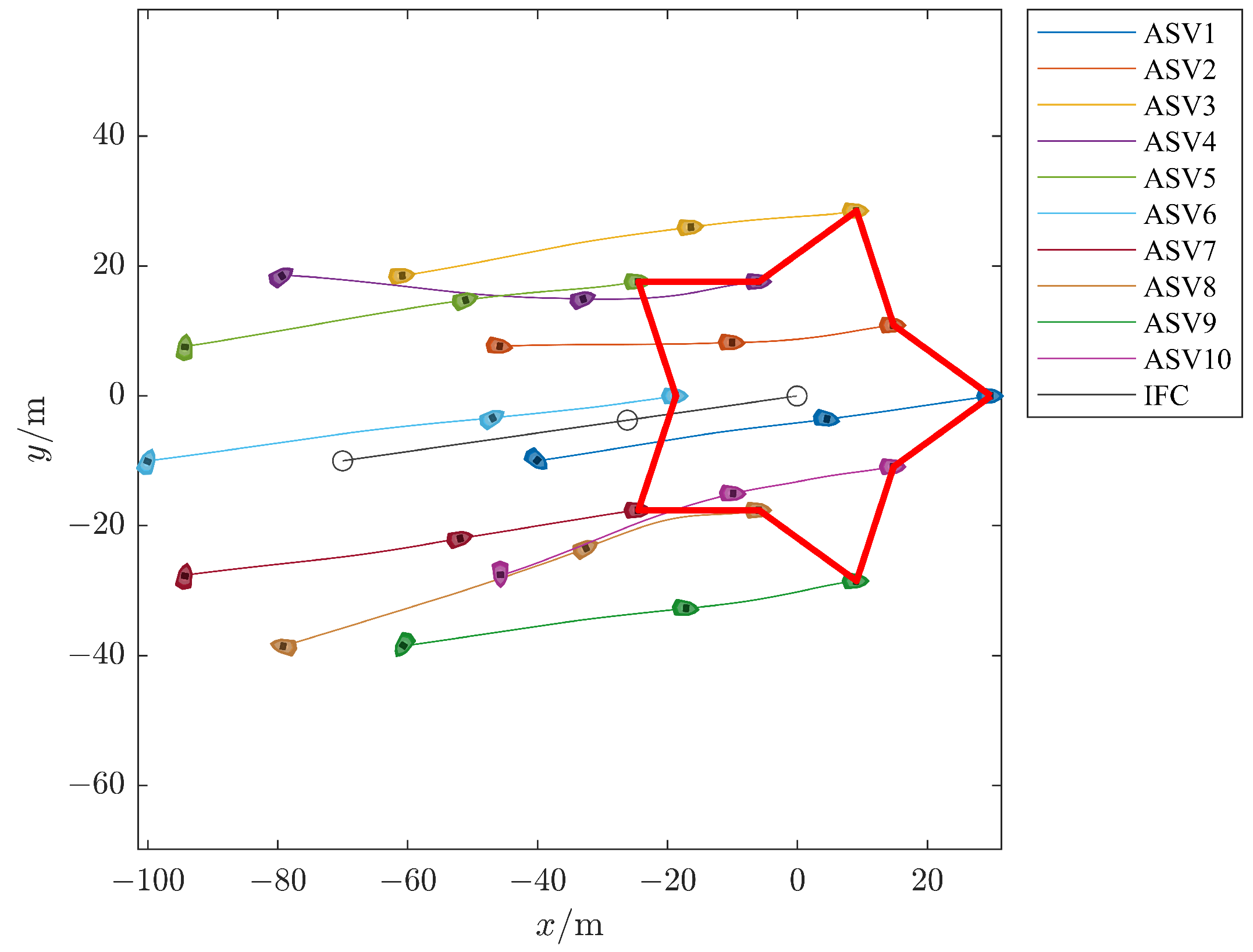
4. Numerical Simulation

In this section, we conducted a leaderless formation simulation involving $N=10$ ASVs and $S=6$ network topologies to verify the effectiveness of the controller. The dynamics parameters in Equation (1) are referenced from [54]. Given the network parameters $T_m=0.9$, $T_d=0.3$, scalar $\delta =10$, $\gamma =5$, ${\lambda }_m=10$, and feedforward gain ${\mathit{K}}_1=\left[\begin{array}{cc}-0.3{\mathbf{I}}_3& -1.5{\mathbf{I}}_3\end{array}\right]$, by solving the LMIs in Theorem 2, the consensus gain is obtained as ${\mathit{K}}_2=\left[\begin{array}{cc}-0.0562{\mathbf{I}}_3& 0.0746{\mathbf{I}}_3\end{array}\right]$. The initial states ${\mathit{\eta }}_i\left(0\right)$ and desired displacements ${\mathit{\alpha }}_i$ are set in

Table 2. Initial parameters in simulation.

Index	${\mathit{\eta }}_{\mathbf{I}}^{\mathit{\top }}\left(0\right)$	${\mathit{\alpha }}_{\mathbf{I}}^{\mathit{\top }}$
1	$\left[\begin{array}{ccc}-40.0& -10.0& -0.7\end{array}\right]$	$\left[\begin{array}{ccc}\phantom{-}30.0& \phantom{-0}0.0& 0.0\end{array}\right]$
2	$\left[\begin{array}{ccc}-45.7& \phantom{-0}7.6& -0.1\end{array}\right]$	$\left[\begin{array}{ccc}\phantom{-}15.0& \phantom{-}10.9& 0.0\end{array}\right]$
3	$\left[\begin{array}{ccc}-60.7& -18.5& \phantom{-}0.1\end{array}\right]$	$\left[\begin{array}{ccc}\phantom{-0}9.3& \phantom{-}28.5& 0.0\end{array}\right]$
4	$\left[\begin{array}{ccc}-79.2& -18.5& \phantom{-}0.5\end{array}\right]$	$\left[\begin{array}{ccc}-\phantom{0}5.7& \phantom{-}17.6& 0.0\end{array}\right]$
5	$\left[\begin{array}{ccc}-94.2& \phantom{-0}7.6& \phantom{-}1.5\end{array}\right]$	$\left[\begin{array}{ccc}-24.3& -17.6& 0.0\end{array}\right]$
6	$\left[\begin{array}{ccc}-99.5& -10.0& \phantom{-}1.2\end{array}\right]$	$\left[\begin{array}{ccc}-18.5& \phantom{-0}0.0& 0.0\end{array}\right]$
7	$\left[\begin{array}{ccc}-94.2& -27.6& \phantom{-}1.4\end{array}\right]$	$\left[\begin{array}{ccc}-24.3& \phantom{-}17.6& 0.0\end{array}\right]$
8	$\left[\begin{array}{ccc}-79.2& -38.5& \phantom{-}2.9\end{array}\right]$	$\left[\begin{array}{ccc}-\phantom{0}5.7& -17.6& 0.0\end{array}\right]$
9	$\left[\begin{array}{ccc}-60.7& -38.5& -2.1\end{array}\right]$	$\left[\begin{array}{ccc}\phantom{-0}9.3& -28.5& 0.0\end{array}\right]$
10	$\left[\begin{array}{ccc}-45.7& -27.6& -1.5\end{array}\right]$	$\left[\begin{array}{ccc}\phantom{-}15.0& -10.9& 0.0\end{array}\right]$

. The environmental disturbance applied during the simulation is configured as $d_{iu}=-2cos\left(0.4t\right)sin\left(t\right)-1.5sin\left(0.5t\right)cos\left(0.5t\right)-2$, $d_{iv}=0.02sin\left(0.1t\right)$, and $d_{ir}=0.5sin\left(1.2t\right)cos\left(0.3t\right)$.

To better illustrate the procedure for obtaining the controller matrix ${\mathit{K}}_2$ and its relevance to subsequent controller implementation, alg:Pcode presents the complete pseudo-code for the i-th ASV given the above parameters. Lines 3–8 demonstrate the use of the fixed-step iterative parameter method to obtain the maximum tolerable values of $T_d$ and $T_m$ within the feasible region of the LMIs, as well as the corresponding controller matrix $K_2$. Lines 9–22 show how the sampled data are utilized during the formation control process and how the ${\mathit{\tau }}_i$ is computed. All simulations were conducted using MATLAB 2022b. The system dynamics were simulated using the Runge–Kutta method (implemented as ode45 in MATLAB), and the LMIs were solved using the MATLAB LMI Toolbox. All computations were performed on an Intel i5-10500 processor.

Algorithm 1: Pseudo-code of the leaderless formation control

1: Inputs: Scalar $\delta$, $\gamma$, matrix ${\mathit{K}}_1$, delay time $T_d$, maximum sampling interval $T_m$, and end time $t_{end}$; 2: Initialize: ASV members $\mathcal{M}$, network topologies ${\left\{G_k\right\}}_{k=1}^S$, desired displacements $\alpha$, initial states ${\mathit{\eta }}_i\left(0\right)$, ${\mathit{\upsilon }}_i\left(0\right)$, start time $t=0$, and indexes $k,l=1$; 3: for$T_{obj}\in \{T_d,T_m\}$do 4:     while the solution of the LMIs in Theorem 2 is feasible do 5:         Update ${\mathit{K}}_2$ by solving LMIs in Theorem 2; 6:         Update $T_{obj}\leftarrow T_{obj}+0.01$; 7:     end while 8: end for 9: while$t<t_{end}$do 10:     for ${\mathrm{ASV}}_i,i\in \mathcal{M}$ do 11:         if the k-th sampling communication occurs at t then 12:            Store $t_k=t$ and ${\mathit{\zeta }}_i\left(t_k\right)$ in the memory; 13:            Broadcast the k-th sampled data ${\mathit{\zeta }}_i\left(t_k\right)$ to its neighbor ASVs; 14:            Update $k\leftarrow k+1$; 15:         end if 16:         if the l-th sampled data of neighbor ASVs are received then 17:            Store $t_l^{\prime }=t$ and ${\mathit{\zeta }}_j\left(t_l^{\prime }\right),j\in {\mathcal{N}}_i$ in memory; 18:            Update $l\leftarrow l+1$; 19:         end if 20:         Compute virtual control ${\tau }_i^{\prime }$ by Equation (11) using l-th sampled data; 21:         Obtain ${\tau }_i$ by inverse transformation ${\tau }_i={\mathrm{\Gamma }}_i^{-1}{\tau }_i^{\prime }$; 22:     end for 23: end while

The simulation results are organized as follows: Figure 5 presents the undirected graphs ${\left\{G_k\right\}}_{k=1}^6$ generated from network topologies. The circles represent the nodes in each graph, and the numbers 1–10 inside the circles indicate the index of each ASV. Figure 6 displays the time-varying topology switching index $k\left(t\right)$. Each step in the plot corresponds to a change in the underlying network topology among the ASVs. This figure reflects the dynamic nature of the communication network, and verifies that the proposed method can maintain formation under such switching conditions. Figure 7 shows the sequence of sampling intervals $T_l$ over time. The intervals are randomly distributed within the admissible range $(0,T_m]$, simulating network-induced aperiodic sampling. This validates the robustness of the control strategy against irregular information updates. Figure 8 illustrates the trajectories of 10 ASVs during the formation process. Each colored curve represents the trajectory of an individual ASV, while the bold red lines highlight the desired pentagram formation defined by the displacement vectors ${\mathit{\alpha }}_{\mathbf{i}}$. The trajectory of IFC is marked in gray, with circular markers denoting key reference points. Notably, the trajectory of the IFC intuitively depicts the overall movement trend of the entire ASV formation. This figure visually demonstrates that all ASVs, starting from dispersed initial positions, successfully converge to and maintain the desired formation pattern, validating the effectiveness of the proposed control strategy under dynamic topology and environmental disturbances. Figure 9, Figure 10 and Figure 11 collectively present the trajectories of consensus errors ${\mathit{\varsigma }}_i-{\mathit{o}}_p$ for all ASVs in the x, y, and $\psi$ components, respectively. It can be observed that, despite initial discrepancies, all error components converge rapidly to neighborhoods around zero. This unified convergence demonstrates that the proposed controller enables the multi-ASV system to synchronize both positions and orientations with the desired displacement, thereby validating the overall effectiveness of the designed controller.

5. Conclusions

In this paper, a leaderless formation controller is proposed for a multi-ASV system, with specific consideration given to the challenges posed by aperiodic sampling communication and data transmission delays. To effectively describe the desired relative positions in the context of a leaderless framework, the concepts of IFC and desired displacements are introduced. This introduction not only simplifies the representation of the expected formation but also lays the foundation for formulating the control objectives of the leaderless formation. By employing a state-space transformation, the problem of achieving the desired formation is reformulated as the stabilization of a subsystem, which provides a more structured approach to analyzing and solving the problem. The effects of delayed and sampled communication are explicitly modeled as time-delay influences within the dynamic system, and the internal stability of the system is rigorously analyzed and proven through the selection of an appropriate LKF. Additionally, the trajectory of the IFC is derived, illustrating the process by which the multi-ASVs achieve leaderless formation. Furthermore, to evaluate the tolerance of the leaderless formation against marine environmental disturbances, an $H_{\infty }$ controller is designed, which significantly improves the system’s ability to maintain formation under uncertain conditions. Finally, the validity and effectiveness of the proposed controller are thoroughly verified through numerical simulations, demonstrating its capability to achieve stable leaderless formation control in the presence of aperiodic sampled communication and data transmission delays.

It should be noted that several assumptions are made in this study to facilitate the theoretical analysis and controller design. For instance, the communication delay is assumed to be bounded and known, the state information of each ASV is considered to be accurately available, and packet loss or communication failures are not explicitly addressed. However, in practical maritime environments, these conditions may not always hold due to unpredictable network delays, sensor noise, or packet dropouts. In future work, we aim to relax these assumptions by investigating more realistic scenarios, such as time-varying and uncertain delays, partial or noisy state measurements, and the presence of packet loss or communication interruptions. Additionally, the extension of the proposed framework to accommodate heterogeneous ASV teams and more complex environmental disturbances will be explored to further enhance the robustness and applicability of the controller in real-world applications.

References

1. Lv, Z.; Wang, X.; Wang, G.; Xing, X.; Lv, C.; Yu, F. Unmanned Surface Vessels in Marine Surveillance and Management: Advances in Communication, Navigation, Control, and Data-Driven Research. J. Mar. Sci. Eng. 2025, 13, 969. [Google Scholar] [CrossRef]
2. Zhang, M.; Liu, Z.; Cai, W.; Yan, Q. Design of Low-cost Unmanned Surface Vessel for Water Surface Cleaning. In Proceedings of the 2021 China Automation Congress (CAC), Beijing, China, 22–24 October 2021; pp. 2290–2293. [Google Scholar] [CrossRef]
3. Ouelmokhtar, H.; Benmoussa, Y.; Benazzouz, D.; Ait-Chikh, M.A.; Lemarchand, L. Energy-based USV maritime monitoring using multi-objective evolutionary algorithms. Ocean Eng. 2022, 253, 111182. [Google Scholar] [CrossRef]
4. Bai, Y.; Wang, Y.; Wang, Z.; Zheng, K. Trajectory Tracking and Docking Control Strategy for Unmanned Surface Vehicles in Water-Based Search and Rescue Missions. J. Mar. Sci. Eng. 2024, 12, 1462. [Google Scholar] [CrossRef]
5. Metcalfe, B.; Thomas, B.; Treloar, A.; Rymansaib, Z.; Hunter, A.; Wilson, P. A compact, low-cost unmanned surface vehicle for shallow inshore applications. In Proceedings of the 2017 Intelligent Systems Conference (IntelliSys), London, UK, 7–8 September 2017; pp. 961–968. [Google Scholar] [CrossRef]
6. Peng, Y.; Yang, Y.; Cui, J.; Li, X.; Pu, H.; Gu, J.; Xie, S.; Luo, J. Development of the USV ‘JingHai-I’ and sea trials in the Southern Yellow Sea. Ocean Eng. 2017, 131, 186–196. [Google Scholar] [CrossRef]
7. Amirkhani, A.; Barshooi, A.H. Consensus in multi-agent systems: A review. Artif. Intell. Rev. 2022, 55, 3897–3935. [Google Scholar] [CrossRef]
8. Zuo, Z.; Liu, C.; Han, Q.L.; Song, J. Unmanned Aerial Vehicles: Control Methods and Future Challenges. IEEE/CAA J. Autom. Sinica 2022, 9, 601–614. [Google Scholar] [CrossRef]
9. Javaid, S.; Saeed, N.; Qadir, Z.; Fahim, H.; He, B.; Song, H.; Bilal, M. Communication and Control in Collaborative UAVs: Recent Advances and Future Trends. IEEE Trans. Intell. Transp. Syst. 2023, 24, 5719–5739. [Google Scholar] [CrossRef]
10. Draganjac, I.; Miklić, D.; Kovačić, Z.; Vasiljević, G.; Bogdan, S. Decentralized Control of Multi-AGV Systems in Autonomous Warehousing Applications. IEEE Trans. Autom. Sci. Eng. 2016, 13, 1433–1447. [Google Scholar] [CrossRef]
11. Chen, X.; Xing, Z.; Feng, L.; Zhang, T.; Wu, W.; Hu, R. An ETCEN-Based Motion Coordination Strategy Avoiding Active and Passive Deadlocks for Multi-AGV System. IEEE Trans. Autom. Sci. Eng. 2023, 20, 1364–1377. [Google Scholar] [CrossRef]
12. Tan, G.; Zhuang, J.; Zou, J.; Wan, L. Multi-type task allocation for multiple heterogeneous unmanned surface vehicles (USVs) based on the self-organizing map. Appl. Ocean Res. 2022, 126, 103262. [Google Scholar] [CrossRef]
13. Chen, C.; Liang, X.; Zhang, Z.; Liu, D.; Li, W. Cooperative strategy based on a two-layer game model for inferior USVs to intercept a superior USV. Ocean Eng. 2024, 293, 116600. [Google Scholar] [CrossRef]
14. Wang, J.B.; Zeng, C.; Ding, C.; Zhang, H.; Lin, M.; Wang, J. Unmanned Surface Vessel Assisted Maritime Wireless Communication Toward 6G: Opportunities and Challenges. IEEE Wirel. Commun. 2022, 29, 72–79. [Google Scholar] [CrossRef]
15. Li, H.; Li, X. Distributed Consensus of Heterogeneous Linear Time-Varying Systems on UAVs–USVs Coordination. IEEE Trans. Circuits Syst. II 2020, 67, 1264–1268. [Google Scholar] [CrossRef]
16. Peng, Z.; Wang, J.; Wang, D.; Han, Q.L. An Overview of Recent Advances in Coordinated Control of Multiple Autonomous Surface Vehicles. IEEE Trans. Ind. Informat. 2021, 17, 732–745. [Google Scholar] [CrossRef]
17. Ghommam, J.; Saad, M.; Mnif, F.; Zhu, Q.M. Guaranteed Performance Design for Formation Tracking and Collision Avoidance of Multiple USVs With Disturbances and Unmodeled Dynamics. IEEE Syst. J. 2021, 15, 4346–4357. [Google Scholar] [CrossRef]
18. Zhang, S.; Zhang, Q.; Xu, L.; Xu, S.; Zhang, Y.; Hu, Y. Dynamic Sliding Mode Formation Control of Unmanned Surface Vehicles Under Actuator Failure. J. Mar. Sci. Eng. 2025, 13, 657. [Google Scholar] [CrossRef]
19. Hu, B.B.; Zhang, H.T.; Liu, B.; Meng, H.; Chen, G. Distributed Surrounding Control of Multiple Unmanned Surface Vessels With Varying Interconnection Topologies. IEEE Trans. Control Syst. Technol. 2022, 30, 400–407. [Google Scholar] [CrossRef]
20. Dong, Z.; Tan, F.; Yu, M.; Xiong, Y.; Li, Z. A Bio-Inspired Sliding Mode Method for Autonomous Cooperative Formation Control of Underactuated USVs with Ocean Environment Disturbances. J. Mar. Sci. Eng. 2024, 12, 1607. [Google Scholar] [CrossRef]
21. Li, J.; Fu, M.; Xu, Y. Disturbance-Observer-Based Adaptive Prescribed Performance Formation Tracking Control for Multiple Underactuated Surface Vehicles. J. Mar. Sci. Eng. 2024, 12, 1136. [Google Scholar] [CrossRef]
22. Li, K.; Xie, S.; Zhang, X.; Zhou, G. A multi-USV Formation Control Method Based on BP Neural Network PID Controller. In Proceedings of the 2024 4th International Conference on Computer, Control and Robotics (ICCCR), Shanghai, China, 19–21 April 2024; pp. 191–195. [Google Scholar] [CrossRef]
23. Zhou, W.; Wang, Y.; Ahn, C.K.; Cheng, J.; Chen, C. Adaptive Fuzzy Backstepping-Based Formation Control of Unmanned Surface Vehicles With Unknown Model Nonlinearity and Actuator Saturation. IEEE Trans. Veh. Technol. 2020, 69, 14749–14764. [Google Scholar] [CrossRef]
24. Wang, D.; Kong, M.; Zhang, G.; Liang, X. Adaptive Second-Order Fast Terminal Sliding-Mode Formation Control for Unmanned Surface Vehicles. J. Mar. Sci. Eng. 2022, 10, 1782. [Google Scholar] [CrossRef]
25. Kheioon, I.A.; Al-Sabur, R.; Sharkawy, A.N. Design and Modeling of an Intelligent Robotic Gripper Using a Cam Mechanism with Position and Force Control Using an Adaptive Neuro-Fuzzy Computing Technique. Automation 2025, 6, 4. [Google Scholar] [CrossRef]
26. Kheioon, I.A.; Saleem, K.B.; Sultan, H.S. Analysis of Natural Convection and Radiation from a Solid Rod Under Vacuum Conditions with the Aiding of ANFIS. Exp. Tech. 2023, 47, 139–152. [Google Scholar] [CrossRef]
27. Bachi, I.O.; Bahedh, A.S.; Kheioon, I.A. Design of control system for steel strip-rolling mill using NARMA-L2. J. Mech. Sci. Technol. 2021, 35, 1429–1436. [Google Scholar] [CrossRef]
28. Ghiaskar, A.; Amiri, A.; Mirjalili, S. Polar fox optimization algorithm: A novel meta-heuristic algorithm. Neural Comput. Appl. 2024, 36, 20983–21022. [Google Scholar] [CrossRef]
29. Jia, H.; Zhou, X.; Zhang, J.; Mirjalili, S. Superb Fairy-wren Optimization Algorithm: A novel metaheuristic algorithm for solving feature selection problems. Clust. Comput. 2025, 28, 246. [Google Scholar] [CrossRef]
30. He, S.; Wang, M.; Dai, S.L.; Luo, F. Leader–Follower Formation Control of USVs With Prescribed Performance and Collision Avoidance. IEEE Trans. Ind. Informat. 2019, 15, 572–581. [Google Scholar] [CrossRef]
31. Lee, J.; Kang, H.; Choi, J.H. A Study on the Improvement of USV’s Leader-Follower Swarm Control Algorithm through Fault Coping Algorithm. In Proceedings of the OCEANS 2023, Limerick, Ireland, 5–8 June 2023; pp. 1–5. [Google Scholar] [CrossRef]
32. Wanniarachchi, C.; Wimalaratne, P.; Karunanayaka, K. Formation Control Algorithms for Drone Swarms and The Single Point of Failure Crisis: A Review. In Proceedings of the 2024 IEEE 33rd International Symposium on Industrial Electronics (ISIE), Ulsan, Republic of Korea, 18–21 June 2024; pp. 1–6. [Google Scholar] [CrossRef]
33. Peng, Z.; Wang, D.; Li, T.; Wu, Z. Leaderless and leader-follower cooperative control of multiple marine surface vehicles with unknown dynamics. Nonlinear Dyn. 2013, 74, 95–106. [Google Scholar] [CrossRef]
34. Zhang, Z.; Huang, B.; Zhou, B.; Miao, J. An Anti-Congestion Interaction Mechanism Based Leaderless Formation Control for Unmanned Surface Vehicles With Communication Interruptions. IEEE Trans. Veh. Technol. 2024, 73, 16964–16976. [Google Scholar] [CrossRef]
35. Wang, S.; Zhang, H.; Baldi, S.; Zhong, R. Leaderless Consensus of Heterogeneous Multiple Euler–Lagrange Systems With Unknown Disturbance. IEEE Trans. Autom. Control 2023, 68, 2399–2406. [Google Scholar] [CrossRef]
36. Hu, B.B.; Zhang, H.T. Bearing-Only Motional Target-Surrounding Control for Multiple Unmanned Surface Vessels. IEEE Trans. Ind. Electron. 2022, 69, 3988–3997. [Google Scholar] [CrossRef]
37. Yu, K.; Li, Y.; Lv, M.; Tong, S. Adaptive Fuzzy Formation Control for Underactuated Multi-USVs With Dynamic Event-Triggered Communication. IEEE Trans. Syst. Man Cybern. Syst. 2024, 54, 7783–7793. [Google Scholar] [CrossRef]
38. Wang, H.; Li, H.; Feng, Y.; Li, Y. Fixed-time coordinated guidance for containment maneuvering of unmanned surface vehicles under delayed communications: Theory and experiment. Ocean Eng. 2023, 277, 114249. [Google Scholar] [CrossRef]
39. Rigatos, G.; Siano, P.; Zervos, N. A nonlinear H-infinity control approach for autonomous navigation of underactuated vessels. In Proceedings of the 2016 16th International Conference on Control, Automation and Systems (ICCAS), Gyeongju, Republic of Korea, 16–19 October 2016; pp. 1143–1148. [Google Scholar] [CrossRef]
40. Fu, T.; Guan, L.; Gao, Y.; Qin, C. An Anti-Windup Method Based on an LADRC for Miniaturized Inertial Stabilized Platforms on Unmanned Vehicles in Marine Applications. J. Mar. Sci. Eng. 2024, 12, 616. [Google Scholar] [CrossRef]
41. Yan, X.; Jiang, D.; Miao, R.; Li, Y. Formation Control and Obstacle Avoidance Algorithm of a Multi-USV System Based on Virtual Structure and Artificial Potential Field. J. Mar. Sci. Eng. 2021, 9, 161. [Google Scholar] [CrossRef]
42. Liu, H.; Weng, P.; Tian, X.; Mai, Q. Distributed adaptive fixed-time formation control for UAV-USV heterogeneous multi-agent systems. Ocean Eng. 2023, 267, 113240. [Google Scholar] [CrossRef]
43. Yuan, P.; Zhang, Z.; Li, Y.; Cui, J. Leader-follower control and APF for Multi-USV coordination and obstacle avoidance. Ocean Eng. 2024, 313, 119487. [Google Scholar] [CrossRef]
44. Zhao, Y.; Ma, Y.; Hu, S. USV Formation and Path-Following Control via Deep Reinforcement Learning With Random Braking. IEEE Trans. Neural Netw. Learn. Syst. 2021, 32, 5468–5478. [Google Scholar] [CrossRef]
45. Fossen, T.I. Handbook of Marine Craft Hydrodynamics and Motion Control; John Wiley & Sons: Hoboken, NJ, USA, 2011; pp. 134–141. [Google Scholar]
46. Knorn, S.; Ahlén, A. Deviation bounds in multi agent systems described by undirected graphs. Automatica 2016, 67, 205–210. [Google Scholar] [CrossRef]
47. Chen, Y.; Chen, C.; Xie, K.; Lewis, F.L. Online Policy Iteration Algorithms for Linear Continuous-Time H-Infinity Regulation With Completely Unknown Dynamics. IEEE Trans. Autom. Sci. Eng. 2024, 21, 6509–6518. [Google Scholar] [CrossRef]
48. Hetel, L.; Fiter, C.; Omran, H.; Seuret, A.; Fridman, E.; Richard, J.P.; Niculescu, S.I. Recent developments on the stability of systems with aperiodic sampling: An overview. Automatica 2017, 76, 309–335. [Google Scholar] [CrossRef]
49. Ge, X.; Han, Q.L.; Zhang, X.M. Achieving Cluster Formation of Multi-Agent Systems Under Aperiodic Sampling and Communication Delays. IEEE Trans. Ind. Electron. 2018, 65, 3417–3426. [Google Scholar] [CrossRef]
50. Petersen, I.R. A stabilization algorithm for a class of uncertain linear systems. Syst. Control Lett. 1987, 8, 351–357. [Google Scholar] [CrossRef]
51. Gu, K. An integral inequality in the stability problem of time-delay systems. In Proceedings of the 39th IEEE Conference on Decision and Control, Sydney, Australia, 12–15 December 2000; Volume 3, pp. 2805–2810. [Google Scholar] [CrossRef]
52. Seuret, A.; Gouaisbaut, F. Wirtinger-based integral inequality: Application to time-delay systems. Automatica 2013, 49, 2860–2866. [Google Scholar] [CrossRef]
53. Park, P.; Ko, J.W.; Jeong, C. Reciprocally convex approach to stability of systems with time-varying delays. Automatica 2011, 47, 235–238. [Google Scholar] [CrossRef]
54. Lu, Y.; Zhang, G.; Sun, Z.; Zhang, W. Adaptive cooperative formation control of autonomous surface vessels with uncertain dynamics and external disturbances. Ocean Eng. 2018, 167, 36–44. [Google Scholar] [CrossRef]
Figure 1. Illustration of the inertial and body-fixed coordinate systems for i-th ASV.
Jmse 13 01259 g001
Figure 2. Illustration of aperiodic sampled communication and transmission delay.
Jmse 13 01259 g002
Figure 3. Flowchart of the main equations and steps in the proposed method.
Jmse 13 01259 g003
Figure 4. Illustration of the operational process of controller within the formation system.
Jmse 13 01259 g004
Figure 5. A collection of undirected graphs { G k } k = 1 6 during the simulation, where (af) correspond to the indices k = 1 , , 6 in sequence. The circles represent the nodes in each graph, and the numbers 1–10 inside the circles indicate the index of each ASV.
Jmse 13 01259 g005
Figure 6. The trajectory of undirected graph index k ( t ) .
Jmse 13 01259 g006
Figure 7. The sampling intervals T l .
Jmse 13 01259 g007
Figure 8. Result of the multi-ASV leaderless formation.
Jmse 13 01259 g008
Figure 9. The trajectory of error ς i x o p x .
Jmse 13 01259 g009
Figure 10. The trajectory of error ς i y o p y .
Jmse 13 01259 g010
Figure 11. The trajectory of error ς i ψ o p ψ .
Jmse 13 01259 g011