
A Study of the Global Buckling Response and Control Measures for Snake-Laid Pipelines Under Uneven Soil Resistances


Abstract
1. Introduction
2. Finite Element Modeling
2.1. Numerical Analysis Models
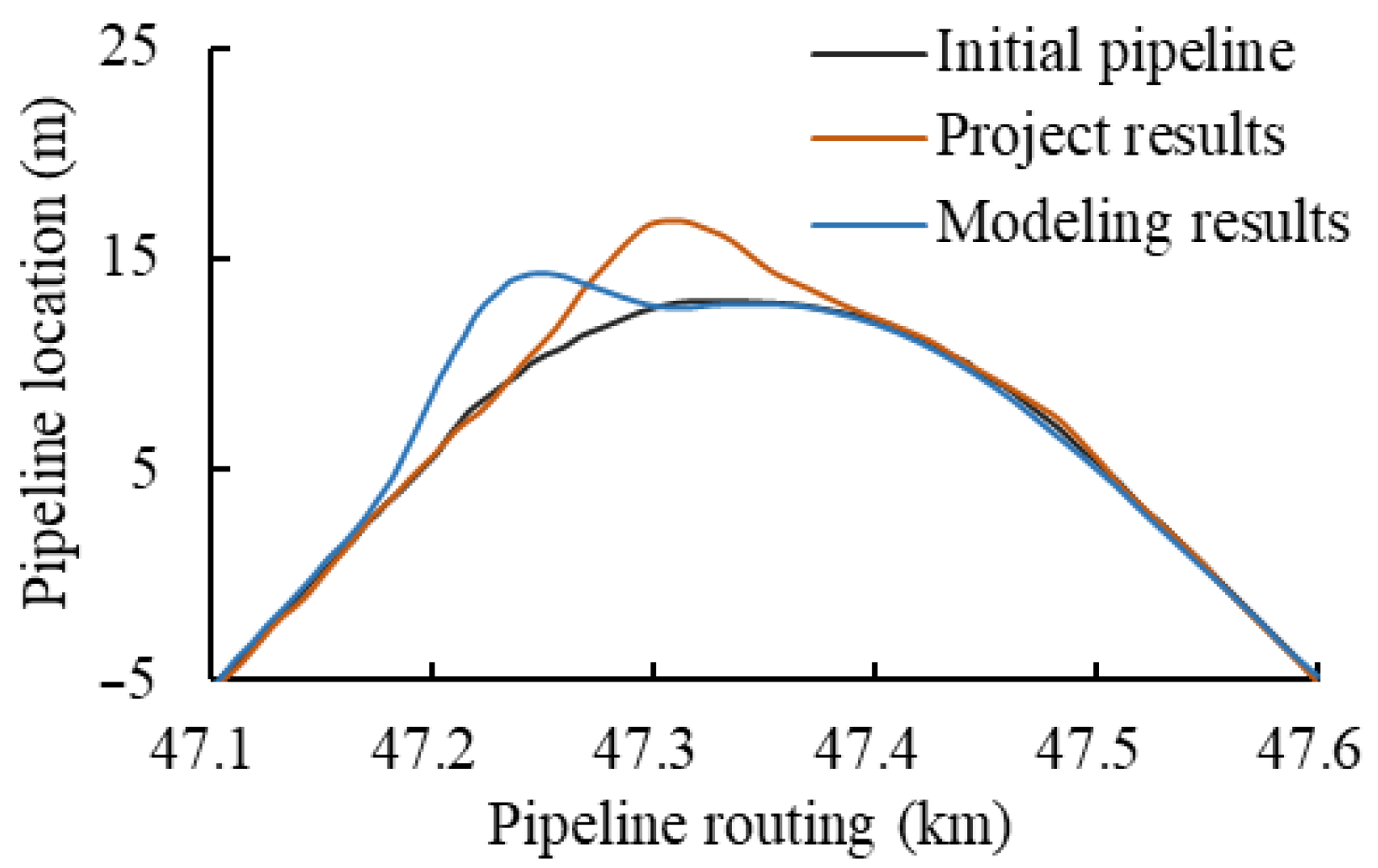
2.2. Model Validation
3. Global Buckling Response of Snake-Laid Pipeline Under Uneven Soil Resistances
3.1. Global Buckling Response of Pipeline Under Different Distribution Gradients of Soil Resistances
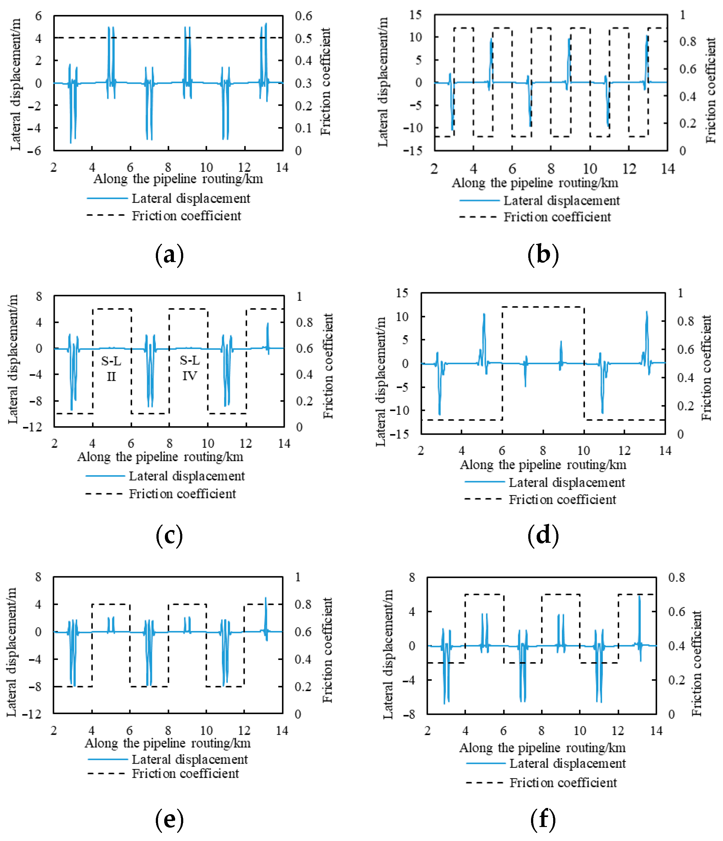
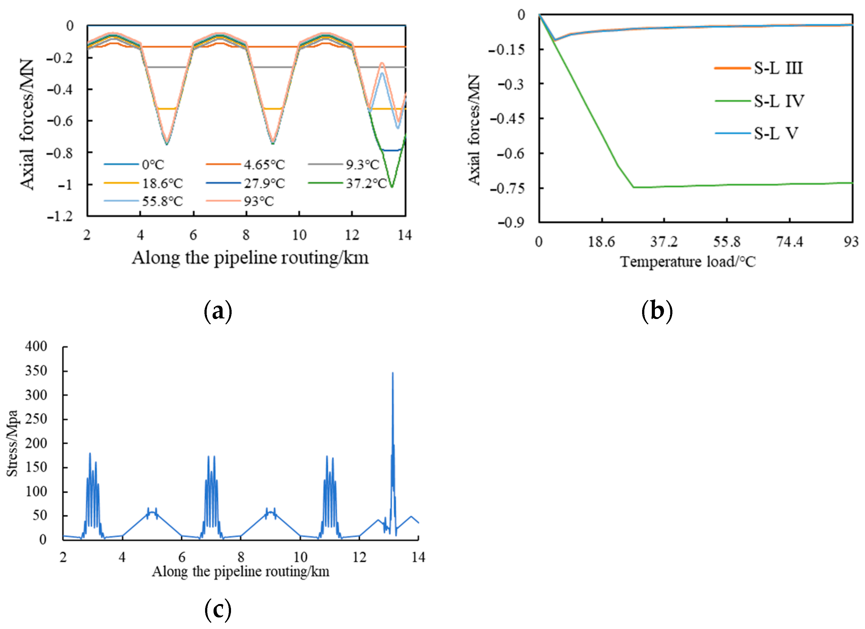
3.2. Global Buckling Response of Pipeline with Different Distribution Patterns of Soil Resistance
4. Study of Snake-Laid Pipeline Scheme Under the Coupling of Uneven Soil Resistance and Snake-Laid Pipeline Parameters
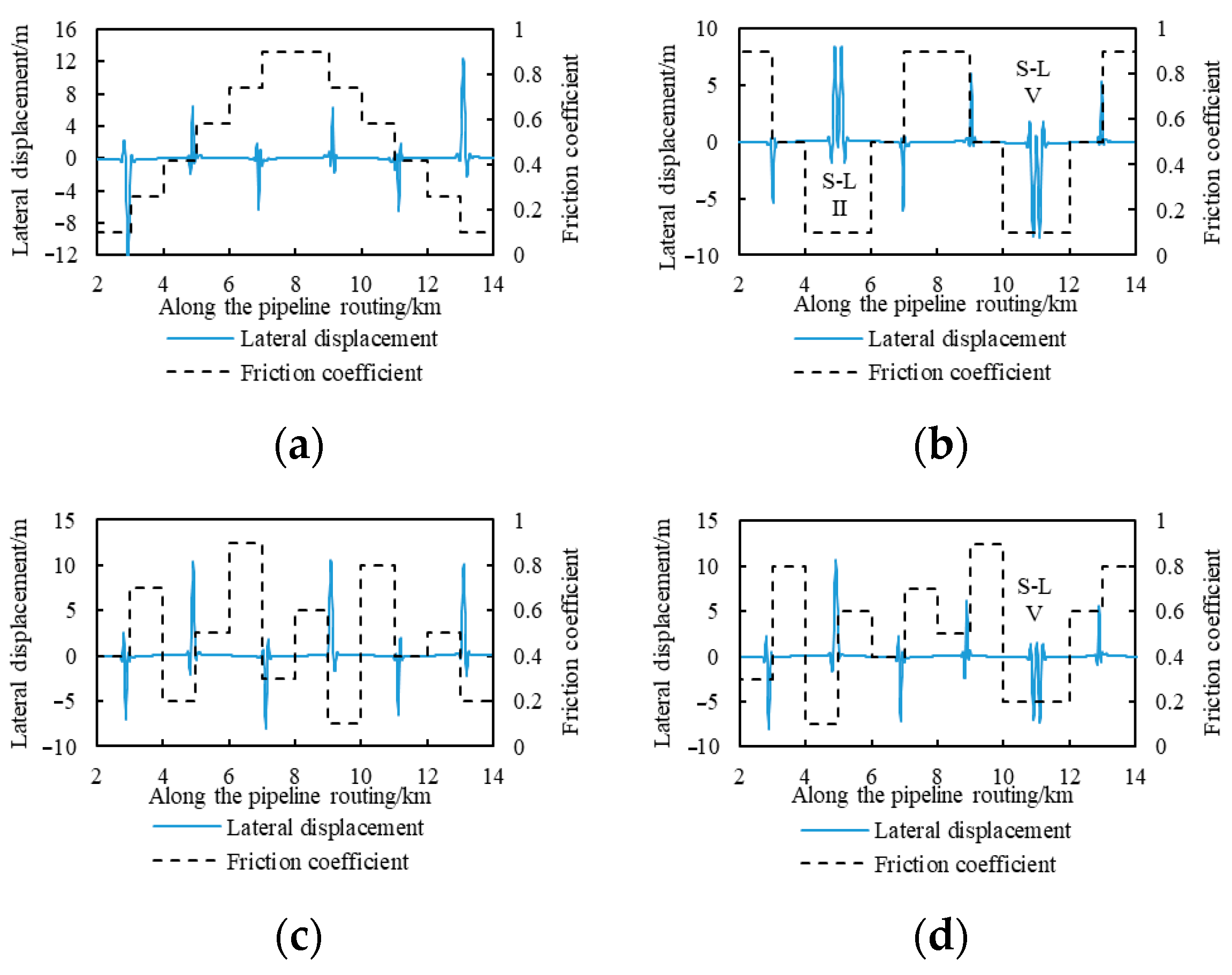
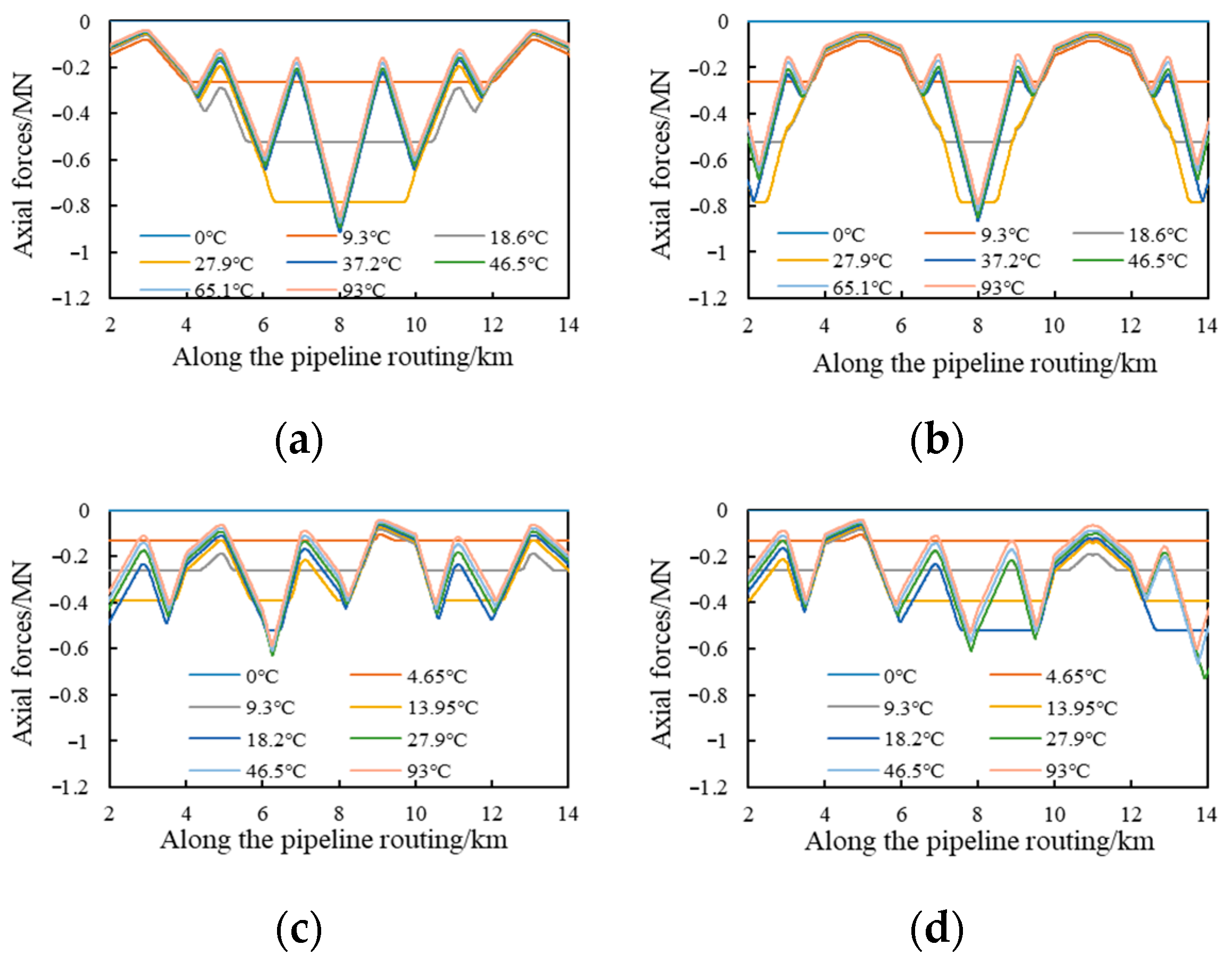
4.1. Global Buckling Response of Snake-Laid Pipelines Under Coupling of Routing Soil Resistance and Snake-Laying Parameters
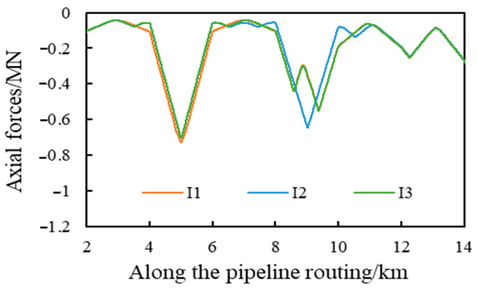
4.2. Determination of Snake-Laying Position Under Random Soil Resistance
5. Discussion
Author Contributions
Funding
Data Availability Statement
Conflicts of Interest
References
- Jukes, P.; Eltaher, A.; Sun, J.; Harrison, G. Extra high-pressure high-temperature (XHPHT) flowlines: Design considerations and challenges. In Proceedings of the International Conference on Offshore Mechanics and Arctic Engineering, Honolulu, HI, USA, 31 May–5 June 2009. [Google Scholar]
- Seyfipour, I.; Walker, A.D. Thermo-mechanical walking of straight and continuous-snake-laid pipelines on sloping seabeds. Appl. Ocean Res. 2020, 94, 101980. [Google Scholar] [CrossRef]
- Wang, Z.; Li, S.; Xu, Q.; He, F. Lateral buckling of subsea pipelines triggered by combined sleeper and distributed buoyancy section. Mar. Struct. 2023, 88, 103343. [Google Scholar] [CrossRef]
- Bai, Q.; Qi, X.; Brunner, M.S. Global Buckle Control with Dual Sleepers in HP/HT Pipelines. In Proceedings of the Offshore Technology Conference, Houston, TX, USA, 4–7 May 2009. [Google Scholar]
- Sævik, S.; Levold, E. High temperature snaking behaviour of pipelines. In Proceedings of the ISOPE International Ocean and Polar Engineering Conference, The Hague, The Netherlands, 11–16 June 1995. [Google Scholar]
- Preston, R.; Drennan, F.; Cameron, C. Controlled lateral buckling of large diameter pipeline by snaked lay. In Proceedings of the ISOPE International Ocean and Polar Engineering Conference, Brest, France, 30 May–4 June 1999. [Google Scholar]
- Hooper, J.; Maschner, E.; Farrant, T. HT/HP pipe-in-pipe snaked lay technology-industry challenges. In Proceedings of the Offshore Technology Conference, Houston, TX, USA, 3–6 May 2004. [Google Scholar]
- Rundsag, J.; Tørnes, K.; Cumming, G.; Rathbone, A.; Roberts, C. Optimised snaked lay geometry. In Proceedings of the ISOPE International Ocean and Polar Engineering Conference, Vancouver, BC, Canada, 6–11 July 2008. [Google Scholar]
- Liu, Y.; Li, X.; Zhou, J.; Song, H. Postbuckling Analysis of Snaked-Lay Pipelines Based on a New Deformation Shape. J. Offshore Mech. Arct. Eng. 2013, 135, 3. [Google Scholar] [CrossRef]
- Wang, Z.; Chen, Z.; He, Y.; Liu, H. Optimized configuration of snaked-lay subsea pipelines for controlled lateral buckling method. In Proceedings of the ISOPE International Ocean and Polar Engineering Conference, Kona, HI, USA, 21–26 June 2015. [Google Scholar]
- Liu, W. Study on snaked laying method and the influence to control lateral buckling. In Proceedings of the IOP Conference Series: Earth and Environmental Science, Beijing, China, 26–28 October 2018. [Google Scholar]
- Cao, Y.; Zhang, S.H.; Sun, L. Numerical research on the effect of snaked-laid pipelines on triggering and controlling lateral global buckling. Ocean Eng. 2019, 37, 39–48. [Google Scholar]
- Seyfipour, I.; Walker, A.; Kimiaei, M. Local buckling of subsea pipelines as a walking mitigation technique. Ocean Eng. 2019, 194, 106626. [Google Scholar] [CrossRef]
- Rezaie, Y.; Sharifi, S.M.H.; Rashed, G.R. Probabilistic fracture assessment of snake laid pipelines under high pressure/high temperature conditions by engineering critical assessment. Eng. Fract. Mech. 2022, 271, 108592. [Google Scholar] [CrossRef]
- Li, T. Study on the Layout Method of Lateral Buckling Snake Laying of Long Oil and Gas Submarine Pipeline. Chem. Ind. Manag. 2023, 9, 165–168. [Google Scholar]
- Liu, R.; Li, C. A Brief History of Lateral Buckling Studies on Submarine Pipelines. J. Tianjin Univ. (Sci. Technol.) 2020, 53, 1–16. [Google Scholar]
- Liu, J.L.; Li, Q.; Yu, H.X. Overview of the offshore pipeline project in the South China Sea sand-wave area and corresponding countermeasures. Pet. Chem. Equip. 2021, 24, 69–74. [Google Scholar]
- Eiksund, G.; Brennodden, H.; Paulsen, G.; Witsø, S.A. Ormen Lange Pipelines—Geotechnical Challenges. In Proceedings of the ISOPE International Ocean and Polar Engineering Conference, Vancouver, BC, Canada, 6–11 July 2008. [Google Scholar]
- Wang, Y. Research on Lateral Soil Resistance of Shallow-Embedded Submarine Pipeline in Sand. Master’s Thesis, Tianjin University, Tianjin, China, 2018. [Google Scholar]
- Shi, R. Global Buckling of Subsea Pipeline and Pipe-Soil Interaction. Ph.D. Thesis, University of Western Australia, Perth, Australia, 2014. [Google Scholar]
- White, D.J.; Westgate, Z.J.; Tian, Y. Pipeline lateral buckling: Realistic modelling of geotechnical variability and uncertainty. In Proceedings of the Offshore Technology Conference, Houston, TX, USA, 5–8 May 2014. [Google Scholar]
- McCarron, W.O. Subsea flowline buckle capacity considering uncertainty in pipe–soil interaction. Comput. Geotech. 2015, 68, 17–27. [Google Scholar] [CrossRef]
- Li, C. Research on Dynamic Response and Mitigation Strategies of Submarine Pipeline Subject to Cyclic Loading of High-Pressure/High-Temperature (HP/HT). Ph.D. Thesis, Tianjin University, Tianjin, China, 2021. [Google Scholar]
- Liu, R.; Xiong, H.; Wu, X.; Yan, S. Numerical studies on global buckling of subsea pipelines. Ocean Eng. 2014, 78, 62–72. [Google Scholar] [CrossRef]
- Matheson, I.; Carr, M.; Peek, R. Penguins flowline lateral buckle formation analysis and verification. In Proceedings of the ASME 2004 International Conference on Offshore Mechanics and Arctic Engineering, Vancouver, BC, Canada, 20 June 2004. [Google Scholar]
- Peek, R.; Matheson, I.; Carr, M. Thermal expansion by lateral buckling: Structural reliability analysis for the penguins flowline. In Proceedings of the ASME 2004 23rd International Conference on Offshore Mechanics and Arctic Engineering, Vancouver, BC, Canada, 20 June 2004. [Google Scholar]


| Density ρ (kg/m3) | Young’s Modulus E (Pa) | Poisson’s Ratio v | Cohesion C (Pa) | Friction Angle φ (°) | Expansion Coefficient α (°C) | |
|---|---|---|---|---|---|---|
| Pipeline | 6007.93 | 2.06 × 10¹¹ | 0.3 | — | — | 1.1 × 10⁻⁵ |
| Seabed | 780 | 3 × 10⁶ | 0.3 | 1800 | 18 | — |
| Condition Number | Type of Soil Resistance Along Pipeline Routing | Distribution of Friction Coefficients Along Pipeline Routing |
|---|---|---|
| A | uniform soil resistance |  |
| B1 | different spacing; the same friction coefficient difference | 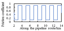 |
| B2 | different spacing; the same friction coefficient difference | 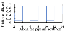 |
| B3 | different spacing; the same friction coefficient difference | 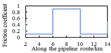 |
| C1 | the same spacing; different friction coefficient differences | 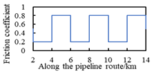 |
| C2 | the same spacing; different friction coefficient differences |  |
| Condition Number | Type of Soil Resistance Along Pipeline Routing | Distribution of Friction Coefficients Along Pipeline Routing |
|---|---|---|
| D1 | uneven symmetric distribution | 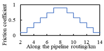 |
| D2 | uneven symmetric distribution | 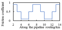 |
| E1 | uneven randomness distribution |  |
| E2 | uneven randomness distribution | 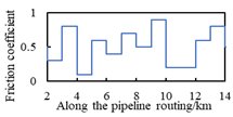 |
| No. | Spacing L (km) | Curvature 1/R (m−1) | Offset w (m) |
|---|---|---|---|
| B2 | 2 | 1/1500 | 92.8 |
| F1 | 1.2 | 1/1500 | 92.8 |
| F2 | 3 | 1/1500 | 92.8 |
| G1 | 2 | 1/1500 | 62.8 |
| G2 | 2 | 1/1500 | 122.8 |
| H1 | 2 | 1/1000 | 92.8 |
| H2 | 2 | 1/2000 | 92.8 |
| NO. | Pipeline Routing by Laying |
|---|---|
| I1 |  |
| I2 |  |
| I3 |  |
Disclaimer/Publisher’s Note: The statements, opinions and data contained in all publications are solely those of the individual author(s) and contributor(s) and not of MDPI and/or the editor(s). MDPI and/or the editor(s) disclaim responsibility for any injury to people or property resulting from any ideas, methods, instructions or products referred to in the content. |
© 2025 by the authors. Licensee MDPI, Basel, Switzerland. This article is an open access article distributed under the terms and conditions of the Creative Commons Attribution (CC BY) license (https://creativecommons.org/licenses/by/4.0/).
Share and Cite
Miao, R.; Sun, X.; Li, C.; Liu, R.; Du, X.; Liu, Y. A Study of the Global Buckling Response and Control Measures for Snake-Laid Pipelines Under Uneven Soil Resistances. J. Mar. Sci. Eng. 2025, 13, 1258. https://doi.org/10.3390/jmse13071258
Miao R, Sun X, Li C, Liu R, Du X, Liu Y. A Study of the Global Buckling Response and Control Measures for Snake-Laid Pipelines Under Uneven Soil Resistances. Journal of Marine Science and Engineering. 2025; 13(7):1258. https://doi.org/10.3390/jmse13071258
Chicago/Turabian StyleMiao, Runnan, Xiang Sun, Chengfeng Li, Run Liu, Xiangning Du, and Yinuo Liu. 2025. "A Study of the Global Buckling Response and Control Measures for Snake-Laid Pipelines Under Uneven Soil Resistances" Journal of Marine Science and Engineering 13, no. 7: 1258. https://doi.org/10.3390/jmse13071258
APA StyleMiao, R., Sun, X., Li, C., Liu, R., Du, X., & Liu, Y. (2025). A Study of the Global Buckling Response and Control Measures for Snake-Laid Pipelines Under Uneven Soil Resistances. Journal of Marine Science and Engineering, 13(7), 1258. https://doi.org/10.3390/jmse13071258