Estimation of Relative Sea Level Change in Locations Without Tide Gauges Using Artificial Neural Networks

Abstract

Sea level rise due to climate change poses an increasing threat to coastal ecosystems, infrastructure, and human settlements. However, accurately estimating sea level changes in regions without tide gauge observations remains a major challenge. While satellite altimetry provides wide spatial coverage, its accuracy diminishes near coastlines. In contrast, tide gauges offer high precision but are spatially limited. This study aims to develop an artificial neural network-based model for estimating relative sea level changes in coastal regions where tide gauge data are unavailable. Unlike conventional forecasting approaches focused on future time series prediction, the proposed model is designed to learn spatial distribution patterns and temporal rates of sea level change from a fusion of satellite altimetry and tide gauge data. A normalization scheme is applied to reduce inconsistencies in reference levels, and Bayesian optimization is employed to fine-tune hyperparameters. A case analysis is conducted in two coastal regions in South Korea, Busan and Ansan, using data from 2018 to 2023. The model demonstrates strong agreement with observed tide gauge records, particularly in estimating temporal trends of sea level rise. This approach effectively compensates for the limitations of satellite altimetry in coastal regions and fills critical observational gaps in ungauged areas. The proposed method holds substantial promise for coastal hazard mitigation, infrastructure planning, and climate adaptation strategies.

1. Introduction

Sea level rise due to climate change poses serious threats to coastal ecosystems, infrastructure, and human safety worldwide [1,2,3]. It leads to various problems such as increased high tide levels, coastal erosion, saltwater intrusion, and inundation of low-lying areas [4,5]. These issues are especially critical in densely populated coastal cities, where sea level rise is closely linked to urban planning, disaster mitigation strategies, and infrastructure design [6]. Accordingly, the ability to accurately estimate the spatiotemporal variations in sea level is increasingly recognized as a key tool for climate change adaptation and sustainable coastal development [7].

Sea level change is generally categorized into global mean sea level rise and relative sea level change [1]. Of these, the relative sea level, experienced directly in coastal areas, is determined not only by ocean surface changes but also by vertical land motion (VLM) [8,9]. For instance, in regions with land subsidence, the relative sea level may rise more sharply than the global average, whereas in uplifting regions, the rise may be mitigated [10]. These characteristics highlight the importance of incorporating VLM into relative sea level estimations, particularly for localized disaster preparedness and adaptive infrastructure planning.

Currently, the two primary methods of sea level observation are tide gauges and satellite altimetry. Tide gauges offer long-term, high-precision sea level measurements at fixed locations, making them suitable for directly monitoring relative sea level changes [11]. However, due to the cost of installation and maintenance, they are not evenly distributed along coastlines, resulting in observational gaps in many areas [12]. In contrast, satellite altimetry provides spatially continuous sea level data across the globe and can complement the spatial limitations of tide gauges [13,14]. Nevertheless, the accuracy of satellite altimetry is known to degrade near coastlines due to factors such as land contamination, complex coastal topography, and electromagnetic interference [15]. While each observation method has its strengths, both are individually limited in their ability to accurately estimate relative sea level changes in coastal regions [16].

Recent studies have actively explored the integration of satellite altimetry and tide gauge data to improve sea level estimations at specific locations [17,18,19,20,21,22]. These efforts aim to combine the wide spatial coverage of satellite altimetry with the high accuracy of tide gauge measurements to better capture sea level variability in coastal zones. For instance, Yang et al. [17] proposed a three-step deep belief network (DBN)-based model for integrating satellite and tide gauge data in the Mediterranean Sea, achieving higher accuracy than conventional interpolation techniques. Zhou et al. [18] employed a long short-term memory (LSTM) neural network to model the time-series characteristics of both data types, enhancing prediction performance. Uebbing et al. [19] improved sea level rise estimation by integrating GNSS-based VLM corrections with tide gauge and satellite data. Raj [20] developed a deep learning prediction model for Kiribati and Tuvalu, demonstrating the feasibility of fusion-based predictions in polar and small island nations. Winona et al. [21] applied an LSTM model to tide gauge data from the Bali coast, successfully capturing both short- and long-term trends. Lastly, Zhao et al. [22] combined Singular Spectrum Analysis with LSTM to model complex sea level variations along the Yellow Sea coast with high precision. While previous studies have significantly advanced sea level prediction by integrating satellite altimetry and tide gauge data, they are often designed for specific regions and depend on long-term, co-located observational records. Moreover, many fusion models emphasize temporal pattern learning and require continuous high-quality data or complex, region-specific configurations, which limits their applicability in data-sparse coastal areas. To overcome these limitations, the present study proposes a more flexible framework that focuses on spatial distribution learning using normalized inputs, thereby enhancing generalizability to ungauged coastal locations.

Building upon this background, the present study proposes an artificial neural net-work (ANN)-based fusion model designed to estimate relative sea level changes at coastal locations lacking tide gauge observations. The model leverages the spatial continuity of satellite altimetry and the precision of tide gauge data to effectively bridge observational gaps in coastal monitoring.

During the training phase, satellite altimetry data from locations with tide gauges are used as input, while data from arbitrary locations without gauges are set as output targets to train the ANN. Although satellite data are globally available, their absolute values are less reliable near coastlines. Therefore, the model is designed to learn the relative spatial distribution of sea level rather than its absolute magnitudes. To this end, all input data are normalized, allowing the network to learn distributional patterns while mitigating reference level discrepancies between the two observation methods.

In the estimation phase, actual tide gauge measurements rather than satellite data are used as model inputs. This enables the model to estimate relative sea level changes at ungauged coastal sites based on real observations from other gauged locations. Despite the difference in input data between training and estimation phases, the model can generalize well due to its emphasis on learning spatial patterns.

This ANN-based estimation framework offers a promising solution for overcoming the limitations of tide gauge coverage and extending the utility of satellite data. A case study was conducted in the Busan area of South Korea, a densely populated area highly vulnerable to sea level rise. The proposed methodology is expected to make meaningful contributions to long-term disaster management planning, coastal infrastructure design, and urban climate adaptation strategies.

2. Data

2.1. Satellite Altimetry Data

In this study, satellite altimetry data were utilized to analyze the spatiotemporal distribution characteristics of sea level. The data were obtained from the Copernicus Marine Environment Monitoring Service (CMEMS), specifically the Global Ocean Ensemble Physics Reanalysis product, which provides global ocean physical variables at a spatial resolution of 0.25° × 0.25° and temporal resolutions of daily or monthly intervals [23]. A total of six years of data, from January 2018 to December 2023, were used in the analysis.

The sea level variable employed was the Sea Surface Height above geoid (SSHa) [23], which represents the elevation of the sea surface relative to the geoid, an equipotential surface that approximates mean sea level. SSHa provides information on the absolute height of the sea surface and differs conceptually from the relative sea level heights measured by tide gauges. It is particularly suitable for analyzing large-scale sea level variations in both open oceans and coastal regions [13].

The reanalysis data used in this study are based on altimeter observations collected by multiple satellite missions, including the Jason series (Jason-2, Jason-3), Sentinel-3A/3B, and SARAL/AltiKa. Satellite altimeters estimate the distance between the satellite and the sea surface by emitting radar pulses and measuring the time it takes for the signal to return. Final sea level heights are derived by applying various corrections for atmospheric delays (troposphere and ionosphere), sea state bias, tides, and other factors [24].

Importantly, the CMEMS altimetry-based reanalysis product used in this study integrates satellite observations with numerical ocean models. Data assimilation techniques such as four-dimensional variational assimilation (4DVAR) and the extended Kalman filter are applied to fill observational gaps and reduce noise, thereby ensuring temporal continuity and spatial consistency of the sea level fields [25]. This integrated reanalysis approach is particularly well-suited for long-term, large-scale sea level analysis.

While satellite altimetry offers the advantage of global spatial coverage, its accuracy tends to decrease in coastal regions. This degradation is attributed to factors such as proximity to shorelines, complex coastal topography, and shallow water depths, which can distort radar signal reflections or introduce land contamination effects [15]. Accordingly, in this study, altimetry data were used not for estimating absolute sea levels at individual points, but rather for learning the relative spatial distribution of sea levels across coastal regions.

During the data preprocessing stage, SSHa values at each grid point within the study domain were extracted sequentially to form a time-series matrix. Invalid or questionable values were removed based on quality flags, and temporal averaging was performed to reduce high-frequency noise. Finally, normalization was applied to prepare the data for input into the learning model, which was then used in estimation experiments.

2.2. Tide Gauge Data

In this study, in addition to satellite altimetry data, tide gauge records were utilized to reflect actual sea level variations in coastal regions. Tide gauges are devices installed on fixed structures such as land-based platforms or breakwaters, continuously measuring the relative height of the sea surface. They provide high-resolution observations of sea level changes at specific fixed locations and are considered one of the most reliable sources for monitoring coastal sea level [26].

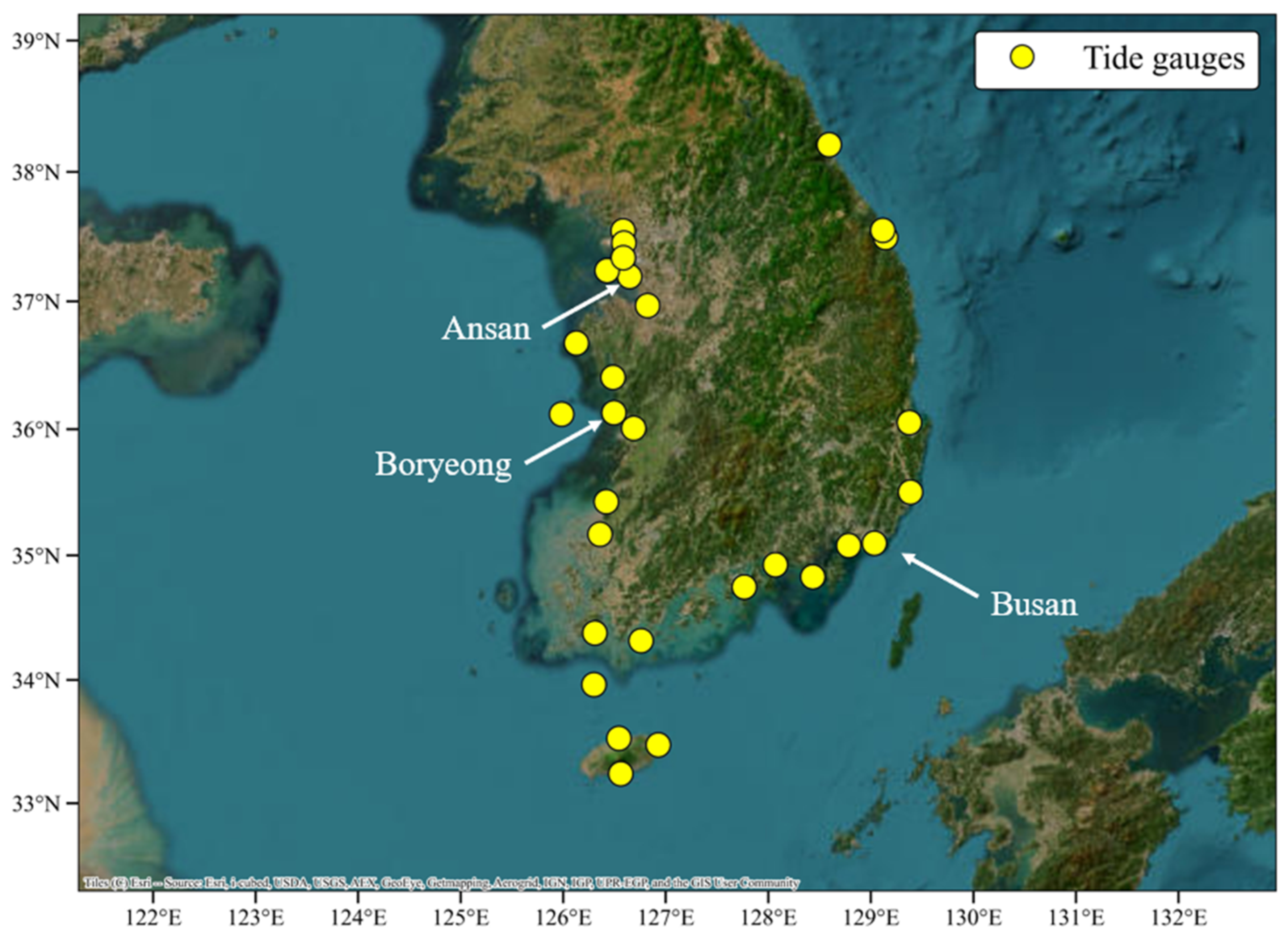
The tide gauge data used in this study were obtained from publicly available ocean observation datasets provided by the Korea Hydrographic and Oceanographic Agency (KHOA) [27]. Data from 34 stations distributed along the entire coastline of South Korea were employed as shown in Figure 1. These data were originally recorded at intervals of 10 min or 1 h and were processed into daily mean values for consistency in analysis.

The preprocessing of the data included a series of quality control steps. First, statistical filtering was applied to remove missing values and outliers from each station’s time series. This multi-step process included the elimination of values exceeding ±3 standard deviations, spike detection based on moving averages, and removal of missing segments identified through the operational history of the stations. To facilitate comparison and integration with satellite altimetry data, the time resolution of all datasets was standardized to daily intervals, and the measurement units and reference surfaces were also harmonized.

Because tide gauges are installed on fixed coastal structures, they offer superior accuracy in measurement location and long-term continuity compared to satellite altimetry. They are especially valuable for capturing localized sea level variations influenced by tides, wind forcing, and ocean circulation, making them widely used as a reliable source of sea level information in coastal areas [7,28]. However, due to their spatial limitations, they lack extensive coverage and are less effective for estimating sea level in offshore or ungauged regions [29].

2.3. Comparison of Sea Level Rise Rates from Satellite Altimetry and Tide Gauge Data

Both satellite altimetry and tide gauges are key observational tools for measuring sea level height; however, due to differences in their physical reference frames and measurement methodologies, they can yield divergent results in long-term trend analyses [30]. To investigate this, the present study calculated 20-year sea level rise rates (from 2003 to 2022) at two coastal locations in South Korea: Busan and Boryeong.

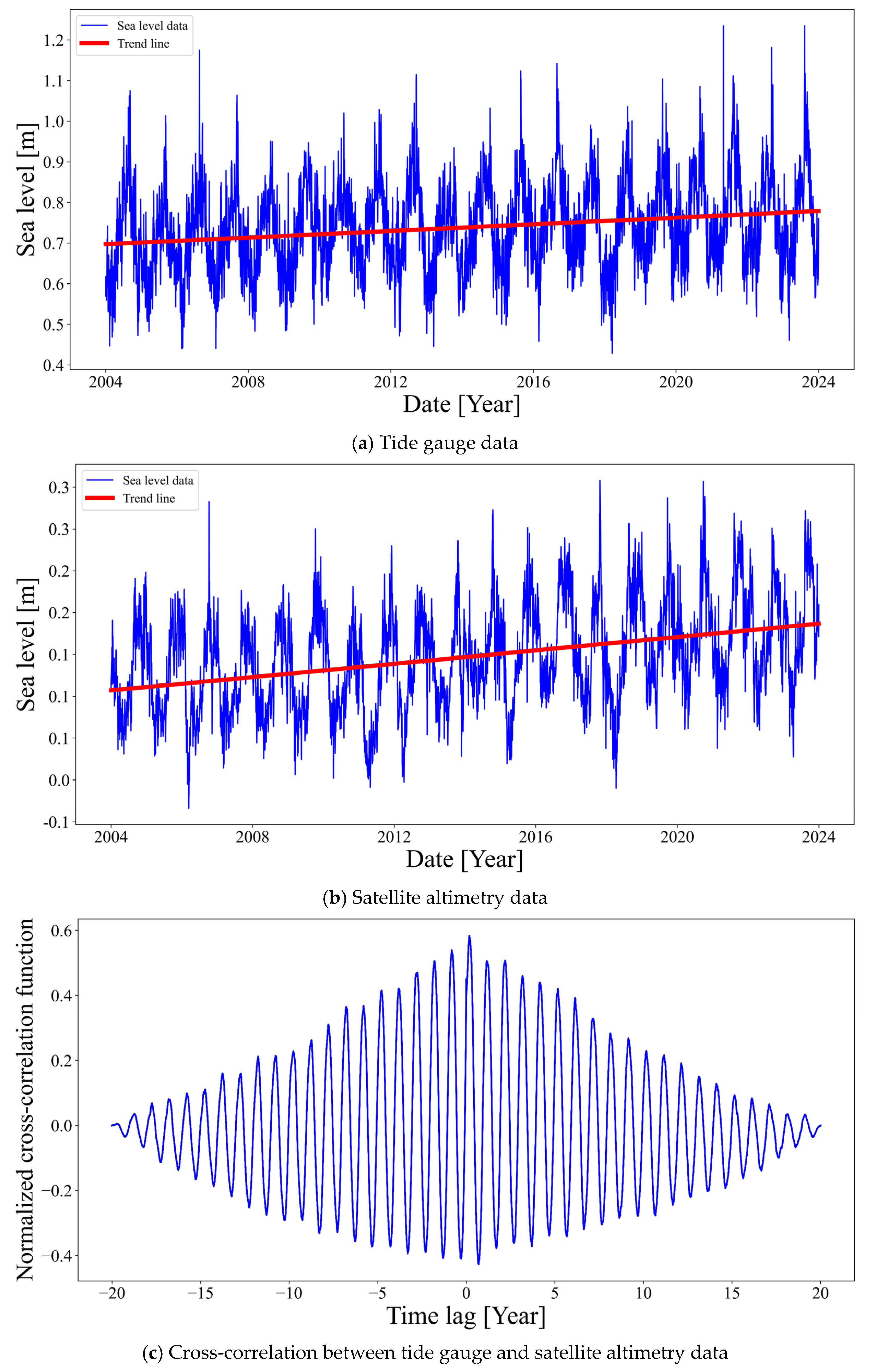
In Busan, as shown in Figure 2, the sea level rise rate derived from tide gauge data was 0.00952 m/year, while that from satellite altimetry was 0.00513 m/year. Figure 2c presents the cross-correlation results between tide gauge and satellite altimetry data for the target region. The analysis indicates that the periodicity of sea level variations is well aligned between the two datasets, as evidenced by the regular pattern of the correlation function. However, the normalized cross-correlation values remain below 0.6, suggesting that although the timing is consistent, the overall correlation strength of the correlation is moderate rather than strong. 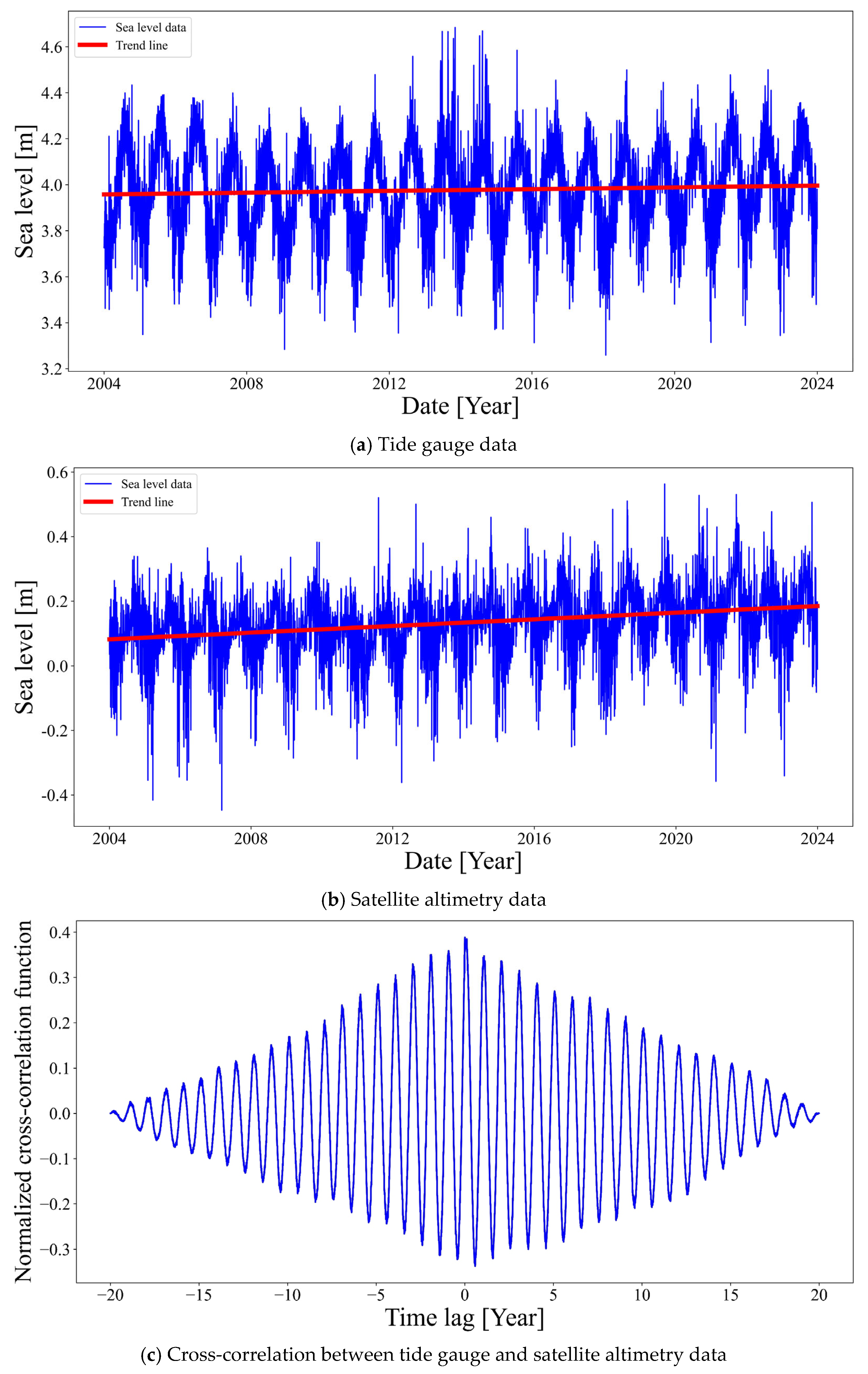At the Boryeong location, as shown in Figure 3, the tide gauge-based rate was 0.0041 m/year, whereas the satellite altimetry-based rate was 0.00571 m/year. Figure 3c presents the cross-correlation results for the Boryeong region. The pattern is comparable to that observed in Figure 2c, indicating aligned periodicity between the tide gauge and satellite altimetry data. However, the normalized correlation values are lower, remaining below 0.4, which suggests a weaker overall correlation strength in this region. These discrepancies in sea level rise rates within the same region are attributed to a combination of factors, including differences in reference surfaces (geoid-based for altimetry vs. land-based for tide gauges), VLM, measurement errors, and disparities in spatial resolution [8].

These results suggest that caution is required when interpreting satellite altimetry data directly in coastal regions or using it for trend analysis at specific locations. In particular, since satellite altimetry measures absolute sea level relative to the geoid, while tide gauges measure relative sea level with respect to the land surface, any vertical land movement (subsidence or uplift) must be considered when comparing trends between the two observation methods.

2.4. Comparison of Spatial Distribution Characteristics Between Satellite Altimetry and Tide Gauge Data

In this section, we compare and analyze the spatial distribution characteristics of sea level based on satellite altimetry and tide gauge data. Using a specific date, 29 May 2023, as a reference, Figure 4a illustrates the spatial distribution of sea level at each location based on tide gauge data, while Figure 4b presents the spatial distribution for the same date derived from satellite altimetry data. Both figures cover the same geographic region and use a consistent coordinate system and circle size representation to facilitate direct comparison. In each figure, sea level values are represented using circle markers, with the full data range divided into five intervals. The size of each circle is scaled proportionally according to its corresponding interval.

A comparison of Figure 4a,b reveals that certain regions exhibit similar patterns of relatively high sea levels across both datasets. However, on a broader scale, the overall spatial distributions show noticeable differences between the two. To assess the relationship between the spatial distributions more objectively, it is necessary to go beyond simple visual comparison and apply quantitative statistical methods. One possible approach is to use matched sea level values from corresponding locations in both datasets and analyze their relationship using techniques such as multivariate nonlinear regression. This enables a more rigorous evaluation of the correlation and estimation consistency between satellite altimetry and tide gauge observations.

3. Methods

This study designed a fusion model based on an ANN to combine the spatial continuity of satellite altimetry with the high-precision sea level measurements of tide gauges. The overall framework consists of two main stages: (1) normalization-based preprocessing for learning spatial distribution patterns and (2) ANN training and estimation using Bayesian optimization.

3.1. Spatial Distribution Normalization

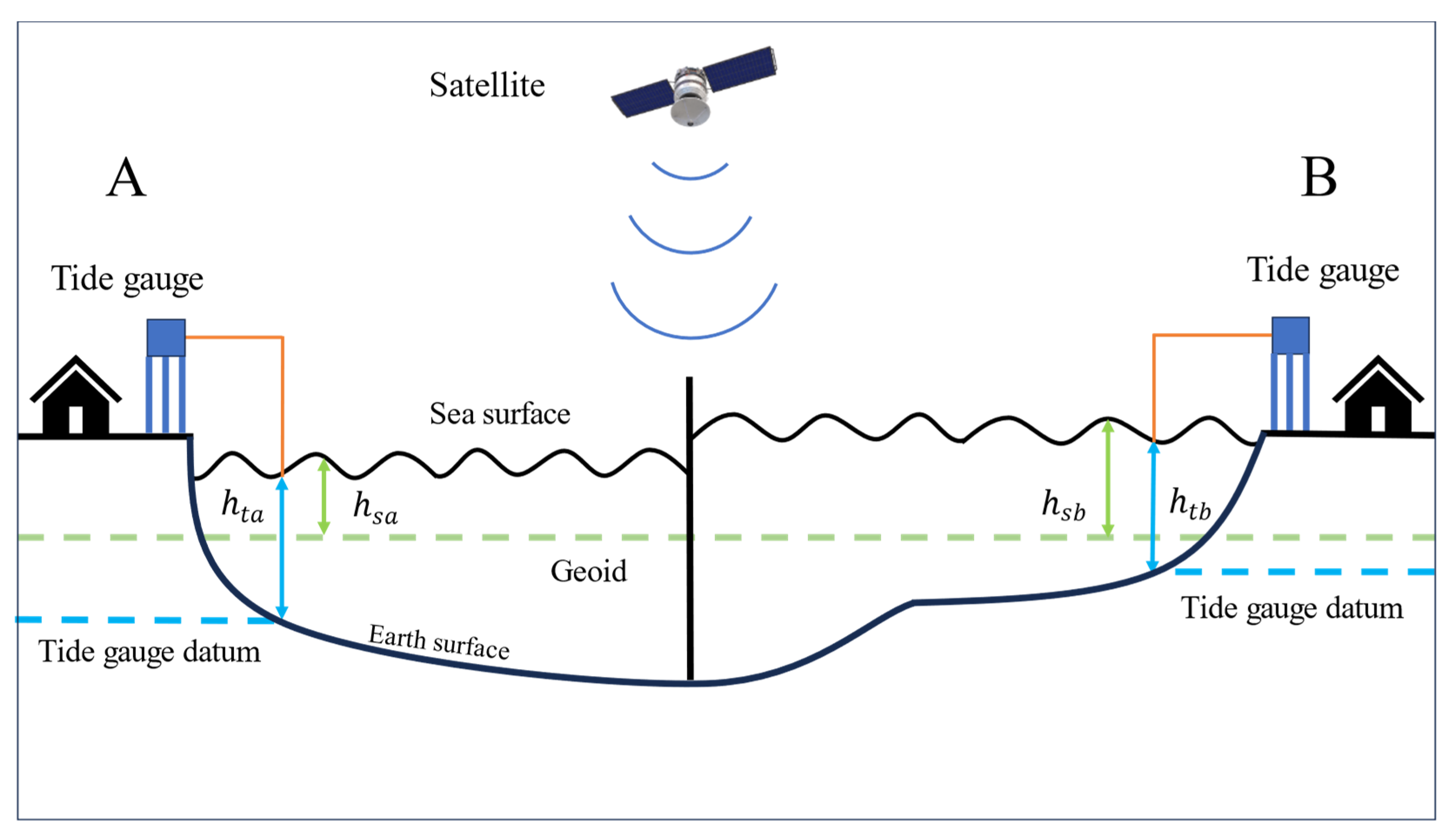
Figure 5 conceptually illustrates the reference surface discrepancy between satellite altimetry and tide gauge observations. The left and right sides of the figure represent two distinct arbitrary regions (Region A and Region B), each depicting the observational configurations of tide gauges and satellite altimeters. Tide gauges measure relative sea level with respect to the local land surface, whereas satellite altimetry measures absolute sea level relative to the geoid using signals received from orbit. As a result, the observed sea level values at the two locations differ in magnitude due to the difference in reference surfaces.

In this study, sea level values at Regions A and B were normalized separately for each observation method using the Z-score approach. This normalization is based on the conceptual framework shown in Figure 5 and is expressed mathematically by Equations (1) and (2).

$$h_{ta}\prime ={\displaystyle \frac{h_{ta}-\mathrm{m}\mathrm{e}\mathrm{a}\mathrm{n}\left(h_{ta},h_{tb}\right)}{\mathrm{s}\mathrm{t}\mathrm{d}\left(h_{ta},h_{tb}\right)}}$$

(1)

where $h_{ta}$ and $h_{tb}$ represent the sea level heights measured by the tide gauge at Regions A and B, respectively. The normalized result based on the mean and standard deviation is denoted as $h_{ta}\prime$.

$$h_{sa}\prime ={\displaystyle \frac{h_{sa}-mean\left(h_{sa},h_{sb}\right)}{std\left(h_{sa},h_{sb}\right)}}$$

(2)

In the same manner, $h_{sa}$ and $h_{sb}$ represent the sea level heights measured by satellite altimetry at Regions A and B, respectively, and the normalized value is denoted as $h_{sa}\prime$.

This normalization approach was applied to the sea level data at all 33 locations considered in this study.

3.2. ANN Modeling and Estimation

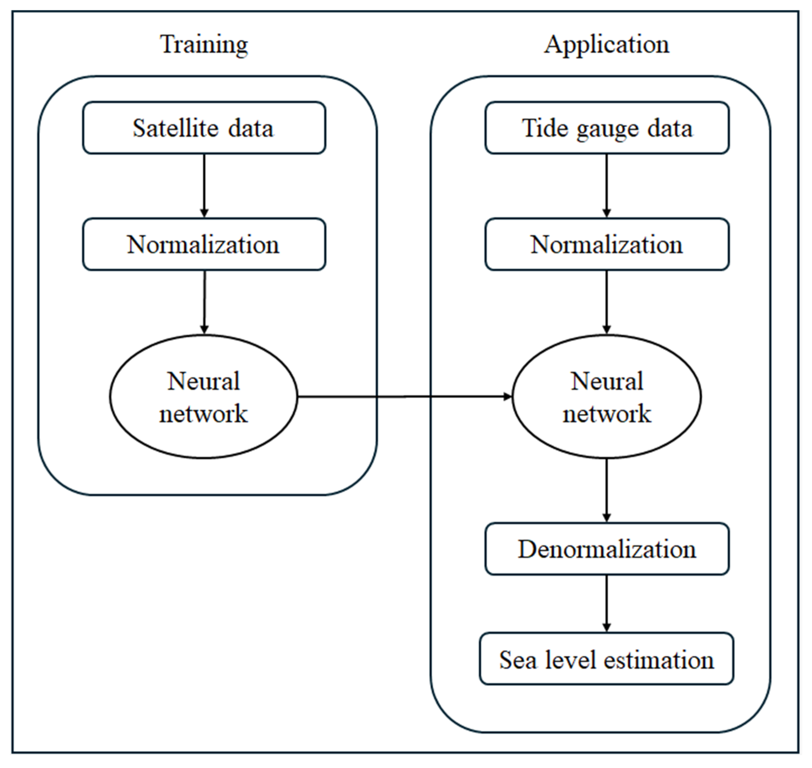
Based on the spatial distribution normalization process described in Section 3.1, this study constructed an ANN model designed to learn spatial distribution patterns of sea level rather than estimate absolute values. The overall training and application procedure is illustrated in Figure 6.

In the training phase, satellite altimetry data for each coastal region were normalized using the Z-score method to eliminate the influence of absolute value deviations caused by differences in reference surfaces. The normalized satellite-based spatial sea level distribution data were then used as inputs to the ANN, enabling the model to learn the relative sea level patterns across the coastal domain.

In the application phase, tide gauge data from the target coastal regions were also normalized using the same Z-score approach and fed into the trained ANN model. Since the ANN was trained to associate satellite-based spatial distributions with tide gauge measurements, it could estimate sea level values at specific locations based on the spatial pattern of tide gauge observations. The estimated outputs were subsequently denormalized to obtain actual sea level values, corresponding to the procedure shown on the right side of Figure 6.

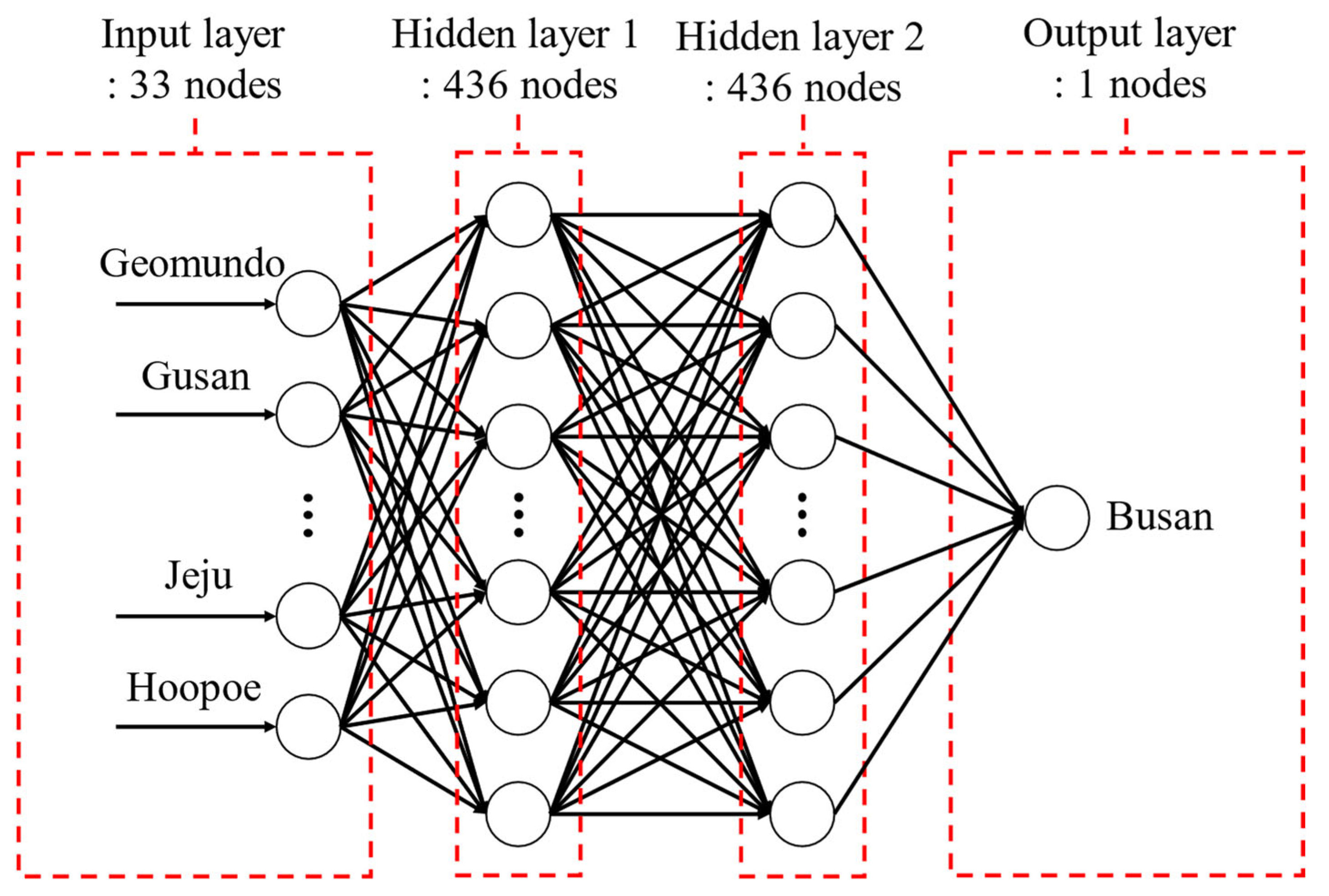
As shown in Figure 7, the structure of the ANN model consists of an input layer with 33 nodes, corresponding to the normalized sea level data from 33 locations, excluding 1 target location (e.g., Busan) out of a total of 34. These input values are passed through 2 hidden layers, each comprising 436 nodes and using the Rectified Linear Unit (ReLU) activation function. The ReLU activation function was selected due to its capability to retain nonlinearity while mitigating the vanishing gradient problem, which often hinders the training of deep networks. It is also computationally efficient and facilitates faster convergence [31]. In the context of this study, where the input space consists of high-dimensional sea level data from 33 tide gauge stations, ReLU contributes to the stability and effectiveness of the learning process. Therefore, it was chosen as a practical and theoretically justified activation function for this application. The final output layer consists of a single node, representing the normalized sea level at the target location.

Among the 34 available locations, data from 33 stations were used as inputs, and the remaining 1 was treated as an unmeasured site to be estimated. During training, it was assumed that tide gauge data were not available at the target site. For the purpose of evaluating estimation performance, the Busan region, where actual tide gauge data exist, was selected as the target. Accordingly, the model was trained to learn the spatial sea level distribution pattern based on the 33 measured sites and then applied to estimate the sea level at the Busan site using only the tide gauge data from the other 33 stations.

This ANN architecture is capable of effectively learning high-dimensional spatial distribution patterns, and the number of nodes and layers in the hidden layers significantly influences the model’s representational capacity and generalization performance. Therefore, in this study, the key hyperparameters of the ANN, including the number of hidden layers, the number of nodes per layer, and the number of training epochs, were automatically determined using Bayesian optimization.

Bayesian optimization is a probabilistic optimization technique based on sequential decision theory, designed to minimize (or maximize) expensive-to-evaluate objective functions. Instead of directly computing the objective function, this method constructs a prior model that estimates the function’s behavior and uses it to efficiently determine the next point to explore. The Bayesian optimization process typically consists of the following three steps [32,33].

1.

Prior Modeling

The objective function $f\left(x\right)$, defined over the hyperparameter space $x$, is modeled using a Gaussian Process (GP). This process is expressed as $f\left(x\right)~GP(m\left(x\right),k\left(x,x^{\prime }\right))$, where $m\left(x\right)$ is the mean function and $k(x,x^{\prime })$ is the covariance (kernel) function. The Gaussian Process provides a predictive distribution over $f\left(x\right)$ based on previously observed data points, allowing estimation of function values at unobserved locations.

2.

Acquisition Function

To select the next candidate point $x$ to evaluate, an acquisition function $a\left(x\right)$ is defined. This function quantifies the expected improvement based on the current predictive distribution, guiding the search toward regions with the highest potential for improvement. One of the most commonly used acquisition functions is the Expected Improvement (EI), which is defined as shown in Equation (3).

$$a_{EI}\left(x\right)=E\left(\mathrm{m}\mathrm{a}\mathrm{x}\right(f_{best}-f\left(x\right)),0)$$

(3)

where $f_{best}$ denotes the minimum value of the objective function observed so far. Using the predictive mean $\mu \left(x\right)$ and standard deviation $\sigma \left(x\right)$ from the Gaussian Process, the Expected Improvement can be computed in closed form, as shown in Equation (4).

$$\begin{array}{c}{a}_{EI}\left(x\right)=\left(f_{best}-\mu \left(x\right)\right)·\mathsf{\Phi }\left(Z\right)+\sigma \left(x\right)·\varphi \left(Z\right)\\ Z={\displaystyle \frac{f_{best}-\mu \left(x\right)}{\sigma \left(x\right)}}\end{array}$$

(4)

where $\mathsf{\Phi }$ denotes the standard normal cumulative distribution function (CDF), and $\varphi$ denotes the standard normal probability density function (PDF).

3.

Optimization and Update

The next candidate point $x_{next}$ is selected by maximizing the acquisition function $a\left(x\right)$. The actual objective function ${f(x}_{next})$ is then evaluated and added to the existing observations to update the Gaussian Process. By repeating this procedure, the algorithm gradually converges toward the optimal value.

In this study, the hyperparameter search space was defined as follows:

-

Number of hidden layers: 1~6;

-

Number of nodes per hidden layer: 4~500;

-

Number of training epochs: 10~1000.

This Bayesian optimization-based hyperparameter selection method enables the identification of high-performing parameter combinations while minimizing the number of iterations required. It is widely recognized as an effective search strategy, particularly in computationally expensive environments.

4. Results

To validate the performance of the proposed estimation method, the trained ANN model was used to estimate sea levels at the Busan location. Normalized sea level values from a total of 33 tide gauge stations were used as input to the model.

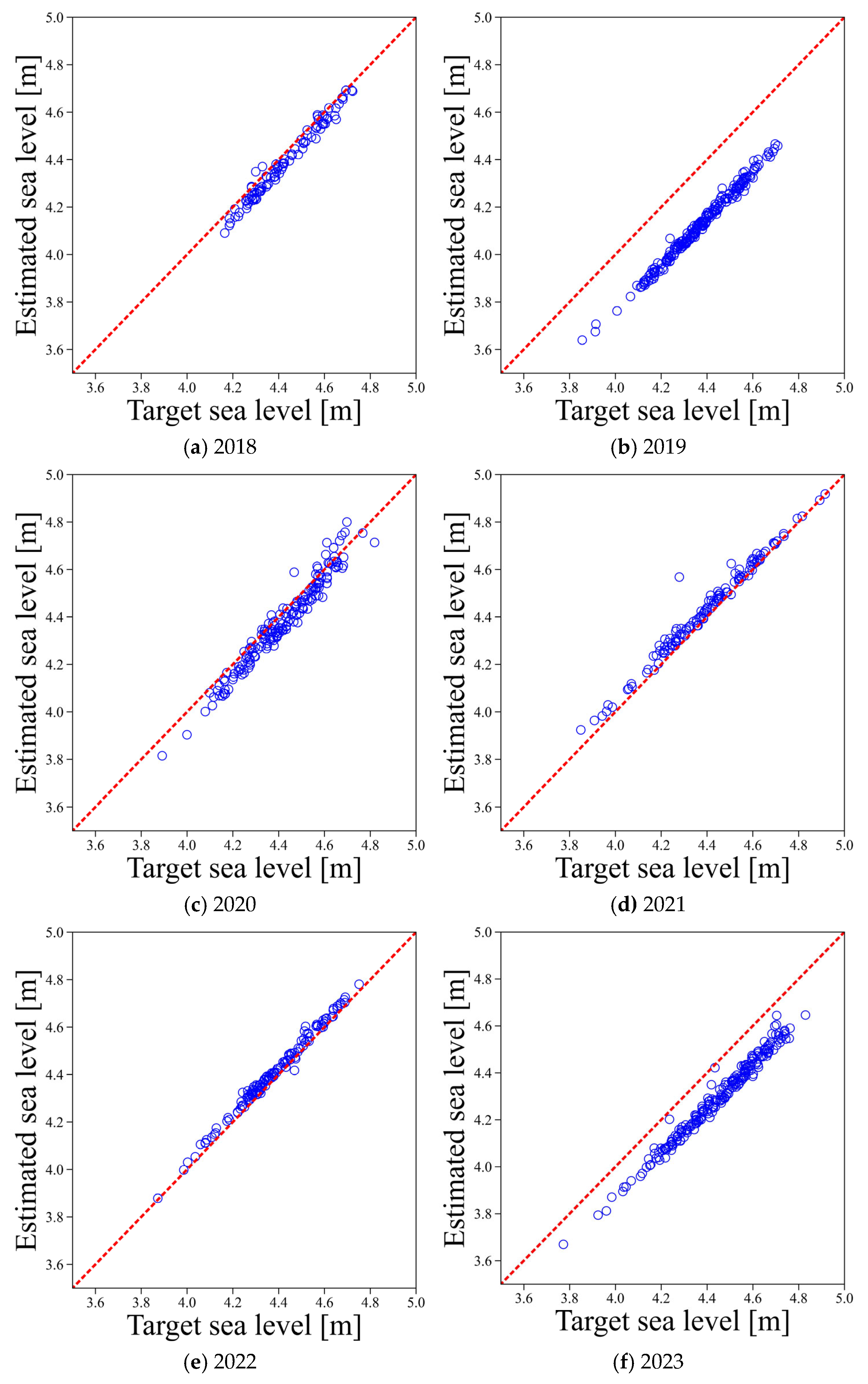
Figure 8 presents a comparison between the estimated sea levels and the actual tide gauge data at the Busan site over the period from 2018 to 2023. The results show that accurate estimation of absolute sea level at ungauged locations is challenging due to the absence of a clearly defined reference surface. However, the estimations exhibited a strong linear relationship with a slope close to one, while each estimation showed a distinct bias. This suggests that although estimating absolute levels may be limited, the model has the potential to effectively capture relative sea level variations over time.

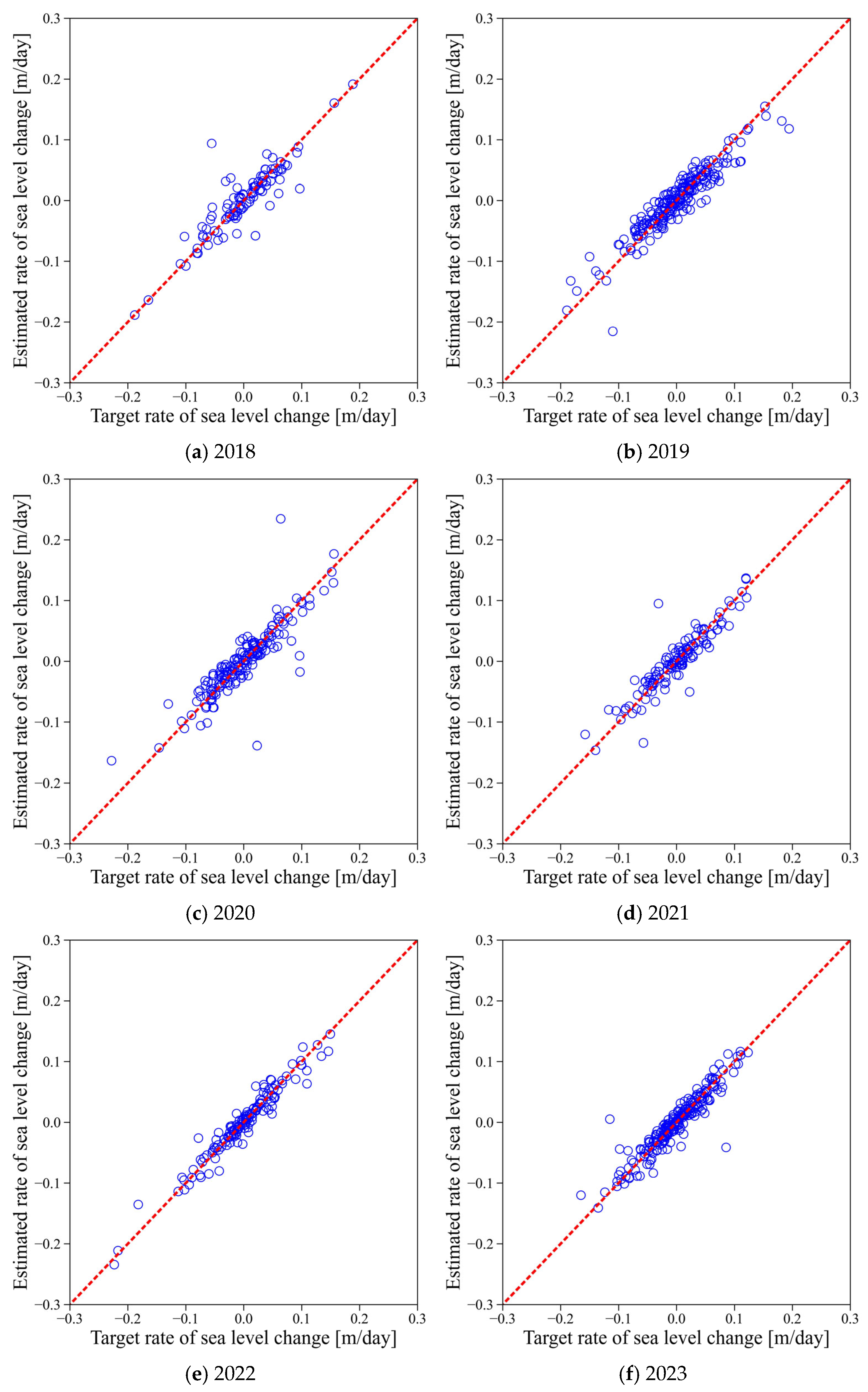
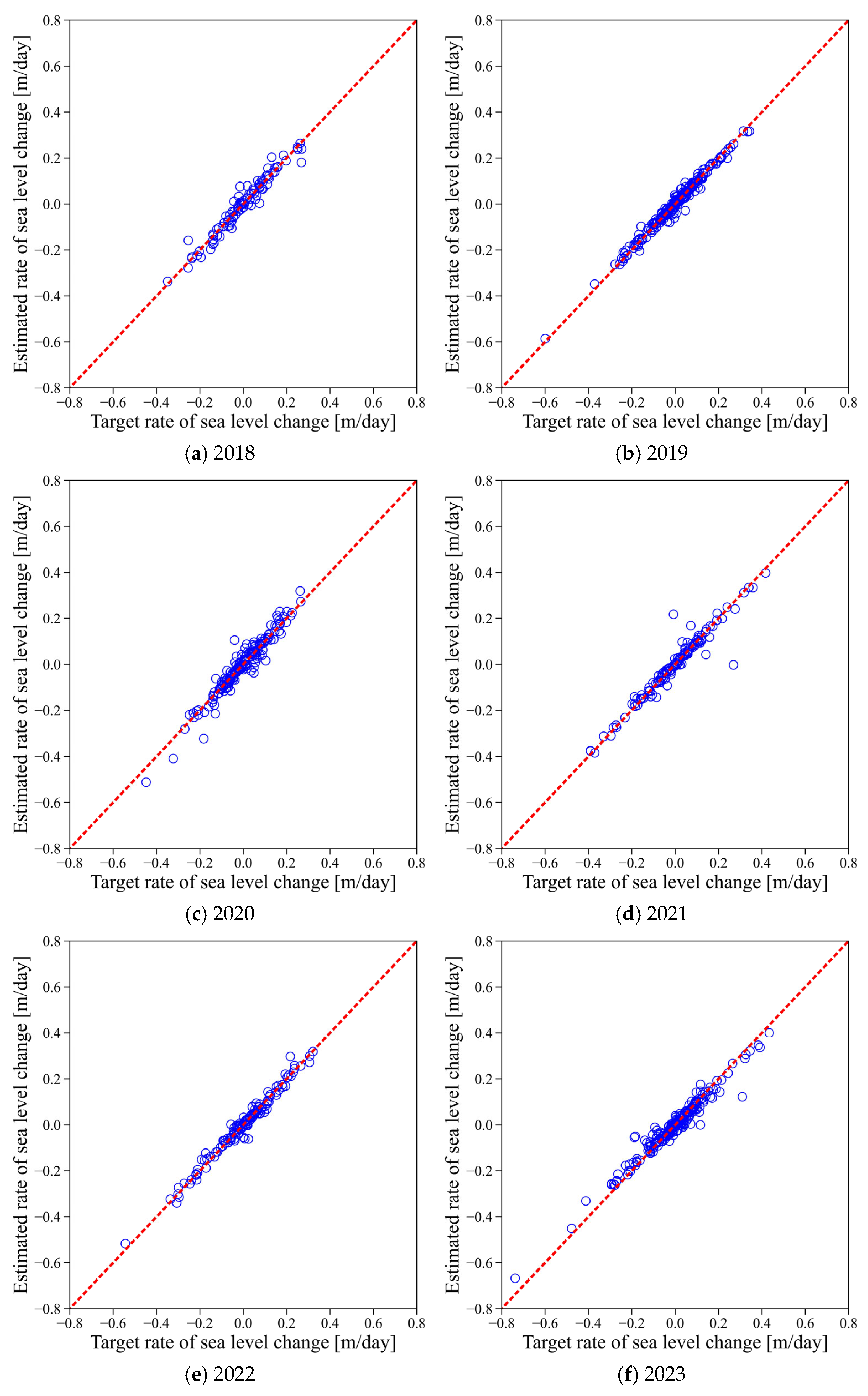
In Figure 9, the daily sea level change rates at the Busan site were computed for each year, and the estimated values were compared with the actual measurements. The bias observed in Figure 8 was not evident here. Although some errors were present, the estimated change rates closely matched the observed rates, indicating that the proposed ANN model can effectively capture temporal trends in sea level changes even at ungauged locations.

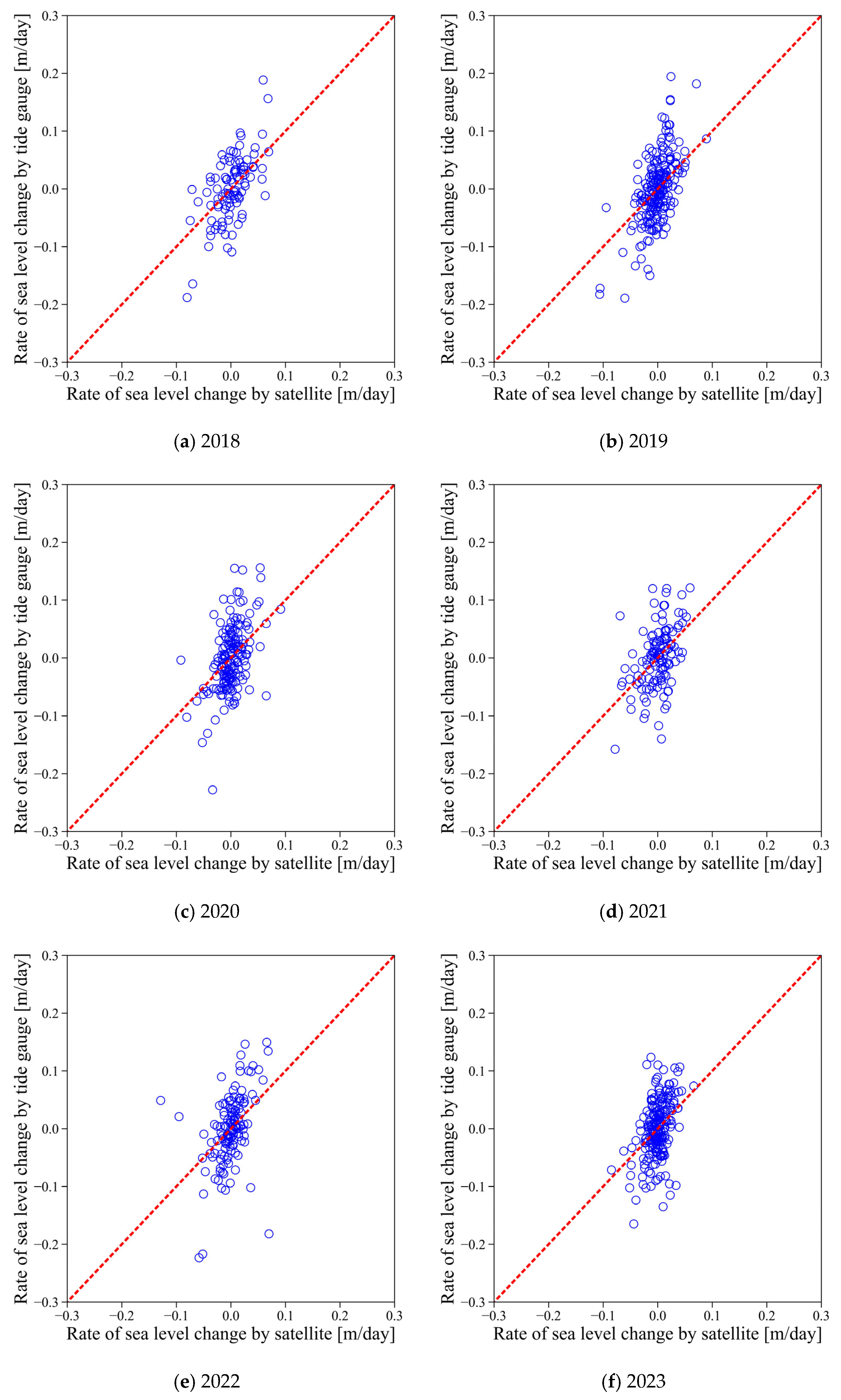
Figure 10 compares sea level change rates at Busan derived from satellite altimetry and tide gauge data over the same period. A significant discrepancy was observed between the two sources, underscoring the limitations of relying solely on satellite data for estimating coastal sea levels. This mismatch highlights the motivation behind this study and emphasizes the need for correctional methodologies to accurately estimate coastal sea level changes.

In this study, the model performance was evaluated through a quantitative comparison between the estimated and observed sea water levels using three indicators: the coefficient of determination (R²), the slope of the linear regression line, and the normalized absolute bias. Each of these metrics offers a distinct perspective on model performance: correlation, scale consistency, and directional bias, respectively, allowing for a complementary and detailed assessment of estimation accuracy.

The coefficient of determination (${\mathrm{R}}^2$) is a widely used metric that evaluates the explanatory power of estimations based on the linear correlation between estimated and observed values. An R² value close to 1 indicates that the estimations account for most of the variance in the observed data, thus serving as a useful measure of overall linear fit. It is computed as shown in Equation (5).

$${\mathrm{R}}^2=1-{\displaystyle \frac{\sum _{i=1}^N{(x_i-y_i)}^2}{\sum _{i=1}^N{(x_i-\overline{x_i})}^2}}$$

(5)

Here, $x_i$ denotes the observed value, $y_i$ is the estimated value, $\overline{x_i}$ is the mean of the observed values, and $N$ is the total number of observations.

The slope obtained by performing linear regression with the estimated values as the dependent variable and the observed values as the independent variable reflects how well the scale of the estimations matches that of the actual values. A slope close to 1 indicates a good scale agreement, while a slope greater than or less than 1 suggests a tendency toward overestimation or underestimation, respectively. Unlike the coefficient of determination, this metric provides information about the proportional relationship between the estimated and observed values. It is calculated as shown in Equation (6).

$$\mathrm{S}\mathrm{l}\mathrm{o}\mathrm{p}\mathrm{e}={\displaystyle \frac{\sum _{i=1}^N(x_i-\overline{x}\left)\right(y_i-\overline{y}) }{\sum _{i=1}^N{\left(x_i-\overline{x}\right)}^2}}$$

(6)

Here, $\overline{y}$ denotes the mean of the estimated values.

Finally, the normalized absolute bias (nABias) is defined as the mean absolute difference between the estimated and observed values, divided by the mean of the observed values. This metric evaluates the average estimation error as a relative proportion. It represents how far, on average, the estimations deviate from the actual values in a normalized form, allowing for an objective comparison of bias across locations with different scales. It is calculated as shown in Equation (7).

$$\mathrm{n}\mathrm{A}\mathrm{B}\mathrm{i}\mathrm{a}\mathrm{s}={\displaystyle \frac{1}{N}}\sum _{i=1}^N\left|{\displaystyle \frac{x_i-y_i}{\overline{x_i}}}\right|$$

(7)

The comparison between the estimated and observed sea levels at the Busan location from 2018 to 2023, as shown in Figure 8, is summarized in

Table 1. Statistical evaluation of estimated vs. observed sea levels at the Busan location (2018–2023).

Year	${\mathbf{R}}^2$	Slope	nABias
2018	0.917	0.832	0.105
2019	0.897	0.847	0.052
2020	0.907	0.821	0.331
2021	0.952	0.887	0.077
2022	0.950	0.938	0.164
2023	0.977	0.955	0.108
Average	0.934	0.880	0.139

. The average ${\mathrm{R}}^2$ was 0.934, indicating that the estimated values explained a high proportion of the variance in the observed data. The average slope between the estimated and observed values was 0.880, suggesting that the model exhibited generally proportional estimation performance with respect to actual sea level variations. In contrast, the nABias was 0.139, indicating that the estimations, on average, deviated from the observed values by more than 13%. Notably, in 2020, the nABias was 0.331, significantly higher than in other years. This may not be solely due to the unknown reference level, but rather the result of unexpected environmental variability, such as anomalous ocean–atmosphere interactions or regional sea level fluctuations that were not reflected in the model inputs. This interpretation is further supported by

Table 2. Statistical evaluation of estimated vs. observed sea level change rates at the Busan location (2018–2023).

Year	${\mathbf{R}}^2$	Slope	nABias
2018	0.784	0.909	0.005
2019	0.880	1.005	0.001
2020	0.773	0.902	0.005
2021	0.846	0.857	0.003
2022	0.944	0.888	0.011
2023	0.871	1.035	0.004
Average	0.850	0.933	0.005

, where the R² for the estimated sea level change rate in 2020 was the lowest (0.773), suggesting that the model may have faced greater challenges in generalizing to the specific conditions of that year.

The comparison between the estimated and observed sea level change rates, as shown in Figure 9, is summarized in Table 2. The average R² was 0.850, indicating that the estimated values generally explained the variance in the actual change rates well. The average slope was 0.933, reflecting a strong linear proportional relationship between the estimated and observed values. Additionally, the nABias was as low as 0.005, confirming that the model estimated sea level change rates with minimal bias.

The comparison of sea level change rates at the Busan location, calculated, respectively, from satellite altimetry and tide gauge data as shown in Figure 10, is summarized in

Table 3. Statistical evaluation of sea level change rates derived from satellite altimetry and tide gauge data at the Busan location (2018–2023).

Year	${\mathbf{R}}^2$	Slope	nABias
2018	0.384	0.324	0.043
2019	0.375	0.257	0.028
2020	0.246	0.180	0.019
2021	0.199	0.217	0.014
2022	0.185	0.188	0.013
2023	0.187	0.166	0.009
Average	0.263	0.222	0.021

. The average R² and slope were 0.263 and 0.222, respectively, indicating very weak correlation and proportionality between the two data sources. However, the nABias was 0.021 on average, suggesting that the results were not particularly biased.

To further assess the generalizability of the proposed model, we applied it to the Ansan location, which was not included in the training process. As shown in Appendix A, Figure A1, the absolute sea level estimations exhibited a certain degree of bias, similar to the results observed at Busan. In contrast, the sea level change rate estimation, presented in Appendix A, Figure A2, showed high accuracy with minimal deviation from the observed values. The quantitative results for sea level estimation and sea level change rate are summarized in Appendix A

Table A1. Statistical evaluation of estimated vs. observed sea levels at the Ansan location (2018–2023).

Year	${\mathbf{R}}^2$	Slope	nABias
2018	0.98	0.953	0.175
2019	0.991	0.99	0.188
2020	0.978	0.945	0.367
2021	0.956	1.075	0.278
2022	0.991	0.987	0.071
2023	0.94	1.031	0.057
Average	0.973	0.997	0.189

and

Table A2. Statistical evaluation of estimated vs. observed sea level change rates at the Ansan location (2018–2023).

Year	${\mathbf{R}}^2$	Slope	nABias
2018	0.957	0.866	0.001
2019	0.978	0.975	0.000
2020	0.933	0.942	0.001
2021	0.932	1.061	0.001
2022	0.982	0.965	0.001
2023	0.949	0.99	0.000
Average	0.955	0.966	0.001

, respectively.

5. Discussion

This study proposes an ANN-based estimation framework that integrates the spatial continuity of satellite altimetry with the high precision of tide gauge measurements, enabling the estimation of sea level information at coastal locations where tide gauges are not installed. Notably, the focus of this study lies in estimating the rate of sea level change rather than the absolute sea level itself, and its effectiveness has been quantitatively validated.

The comparison between estimated and observed values showed that while the model demonstrated high explanatory power in estimating absolute sea levels, a certain level of bias was present. In the case of the Busan site, the average R² was 0.934, and the regression slope was 0.880, indicating that the estimated sea level closely followed the observed trend. However, the nABias was 0.139, meaning that the estimations deviated from the actual values by more than 13% on average. This bias may be attributed to various factors, including differences in reference levels, regional characteristics, and the absence of VLM correction. These results suggest that there are structural limitations in estimating absolute sea levels, and caution should be exercised when applying this method for precise sea level estimation in unmeasured regions.

In contrast, the model showed excellent performance in estimating sea level change rates. From 2018 to 2023, the estimated change rates at the Busan site exhibited a strong correlation with the observed values, with an average R² of 0.850, a slope of 0.933, and a negligible bias of 0.005. These results indicate that the Z-score normalization technique effectively captured the relative temporal variation patterns and that the proposed approach is more suitable for estimating trends than absolute values.

Furthermore, sea level change rates derived solely from satellite altimetry showed significant discrepancies compared to those derived from tide gauge data (R² = 0.263, slope = 0.222). This highlights the limitations of relying solely on satellite data in coastal regions and underscores the necessity of complementing satellite observations with tide gauge data for reliable estimation of sea level trends.

While the proposed method demonstrated reliable performance in two regions of Korea, where tide gauge stations are densely distributed and spatial correlations are strong, its applicability to more complex geographical environments remains to be explored. To improve the model’s generalizability, future work should focus on developing advanced input selection and correction strategies that can effectively capture localized spatial variability. Furthermore, comparative analysis with physically based reanalysis products such as GLORYS would be valuable in assessing the relative strengths of data-driven versus physics-driven approaches, especially in observation-sparse coastal regions. Overall, this study presents a model structure and data preprocessing strategy that are more suitable for estimating temporal trends in sea level rather than reproducing absolute sea level values. The proposed framework shows promise as a practical decision-support tool for coastal disaster response, infrastructure planning, and the optimization of ocean observation systems.

6. Conclusions

This study proposed a methodology for estimating sea level information in coastal areas without tide gauges by employing a satellite-tide gauge fusion estimation model based on ANNs. The core contribution of this work lies in its development of an approach that focuses on accurately estimating sea level change rates, rather than absolute sea level values.

The Z-score-based spatial normalization technique effectively eliminated differences in reference levels and regional discrepancies, while Bayesian optimization was employed to maximize the generalization performance of the ANN model. The resulting estimation model showed some degree of bias in estimating absolute sea levels (nABias = 0.139), indicating limitations in achieving fully precise estimations. However, for sea level change rates, the model demonstrated excellent performance, with an average coefficient of determination of 0.850, a regression slope of 0.933, and a minimal bias of 0.005.

These findings suggest that the proposed model is particularly well suited for time-series-based trend analysis and change detection of sea level, rather than for estimating instantaneous sea level heights. Consequently, the model offers more practical utility in applications such as diagnosing the impacts of climate change on coastal zones, formulating urban disaster prevention plans, and developing early warning systems for marine hazards.

Future research will focus on verifying the model’s generalizability through applications to a wider range of coastal locations, including more complex geographical settings. Additionally, integrating environmental factors such as climate indices, land deformation, wind, and atmospheric pressure as input variables could further enhance the model’s estimation reliability. The development of a hybrid model combining both temporal and spatial estimation capabilities may also open new directions for sea level forecasting research.

In conclusion, this study presents a quantitative and practical solution for estimating sea level change rates, going beyond the limitations of absolute sea level estimation. The proposed framework has the potential to fill information gaps in coastal regions and support sustainable ocean management and disaster prevention strategies.