Semi-Supervised Maritime Object Detection: A Data-Centric Perspective

Abstract

Semi-supervised object detection (SSOD) has emerged as a promising technique to boost the performance of the detectors, utilizing both labeled and unlabeled data. However, in marine environments, SSOD faces formidable challenges posed by complex conditions like shore-based landscapes, varying ship scales, and diverse weather, which complicate data acquisition and thus the generation of accurate pseudo-labels. To tackle these issues, we propose two novel strategies, depth-aware pseudo-label filtering (DAPF) and dynamic region mixup (DRMix) augmentation, from a data-centric perspective. Specifically, the DAPF strategy incorporates depth information as a prior to refine pseudo-labels by filtering out unreliable ones, thereby improving the quality of pseudo-label–data pairs used for training. Meanwhile, DRMix augmentation dynamically mixes images at the regional level, generating diverse and representative data suitable for maritime object detection tasks. Extensive experiments on maritime datasets validate the effectiveness of our approach, achieving mAP improvements of 2.2% on the SeaShips dataset and 0.9% on the Singapore Maritime dataset compared to other state-of-the-art (SOTA) methods. Our code will be made publicly available.

1. Introduction

Maritime object detection is crucial for unmanned surface vehicles (USVs), which play a significant role in autonomous navigation, maritime surveillance, and water quality monitoring. The primary objective is to accurately locate and classify objects of interest, such as ships, buoys, debris, and marine life, under complex maritime conditions. With the rapid advancement of neural networks, vision-based maritime object detection has gained increasing attention and has demonstrated promising results [1,2,3,4,5,6].

Deep learning-based object detection has achieved remarkable progress. This includes convolutional neural network (CNN)-based methods, such as one-stage detectors [7,8,9] and two-stage detectors [10,11,12], as well as more recent transformer-based methods [13,14]. However, these models typically require large-scale annotated datasets to achieve high performance due to their complex architectures with numerous trainable parameters. For maritime applications, collecting and annotating such datasets is both time-consuming and expensive. Moreover, real-world maritime environments introduce further complications, such as occlusions, scale variations, illumination changes, and cluttered backgrounds, making accurate data labeling even more difficult. These challenges highlight the need for methods that can effectively leverage both labeled and unlabeled maritime data.

Semi-supervised object detection (SSOD) [15,16,17,18] has emerged as a promising solution to reduce the dependency on extensive labeled datasets by utilizing abundant unlabeled data. Most SSOD methods adopt techniques like pseudo-labeling and consistency regularization within a teacher–student framework to achieve high detection accuracy. These approaches have demonstrated state-of-the-art (SOTA) performance on general object detection benchmarks like COCO [19]. However, directly applying SSOD to maritime scenarios poses unique challenges due to the highly dynamic and complex nature of marine environments. A key issue is the generation of low-quality pseudo-labels, often caused by false positives and missed detections in complex maritime scenes. This can significantly degrade the overall detection performance. For instance, applying SOTA methods like ARSL [15] to maritime datasets (e.g., the Singapore Maritime Dataset (SMD) [20]) has resulted in obvious performance degradation, as shown in Figure 4. We attribute this to the inherent limitations of the existing SSOD framework within the maritime domain. In particular, the teacher model tends to produce noisy and unreliable pseudo-labels under maritime conditions, which increases the likelihood of false positives (detecting non-existent objects) and false negatives (missing real objects). When these erroneous pseudo-labels are used to train the student model, they introduce harmful noise into the learning process, ultimately reducing detection accuracy and model robustness. Therefore, a critical objective in maritime SSOD is to improve pseudo-label quality, i.e., to retain more true positives while effectively filtering out false positives, to ensure more reliable and robust learning.

Additionally, SSOD methods benefit from data augmentation techniques like Mixpl [16], which extends mixup [21] by linearly combining pseudo-labeled images. However, these mixup-based methods treat object detection as an image-level task rather than a region-level one, which is suboptimal given that object detection inherently focuses on specific regions of interest. This limitation becomes particularly problematic in maritime imagery, where complex backgrounds and blurry object boundaries are prevalent. Naively mixing entire images can result in the blending of object regions with incompatible background contexts, producing unrealistic and distorted features. These artifacts may lead to confusing and misleading training samples that violate the core principle of consistency regularization. As a result, the model’s ability to learn robust and discriminative representations for maritime objects is significantly compromised.

To address the aforementioned challenges, we propose two novel strategies for SSOD in maritime environments, with a focus on data preparation:

• A depth-aware pseudo-label filtering (DAPF) strategy: In maritime scenes, object depth and scale are often strongly correlated within specific categories due to the open and unobstructed nature of the environment. To leverage this property, we introduce depth information as a regularization signal to improve the reliability of pseudo-labels. By modeling the joint distribution of object depth and scale, the DAPF strategy effectively utilizes depth priors to filter out low-confidence or inconsistent pseudo-labels.
• Dynamic region mixup (DRMix) augmentation: Given the complexity of maritime scenes, we propose an adaptive mixup augmentation technique that operates at both image and region levels. The image-level component dynamically adjusts fusion weights according to training difficulty, while the region-level component introduces an object-aware augmentation tailored specifically for detection tasks, mitigating the adverse effects of naive image blending in visually complex maritime scenes.

These two data-centric strategies, targeting pseudo-label refinement and augmentation, are designed to fully exploit the potential of unlabeled data for SSOD in maritime scenarios, a relatively under-explored area in current research.

2. Related Works

2.1. Object Detection

Fully supervised object detection methods are broadly categorized into two-stage and one-stage detectors. Two-stage detectors, such as Faster R-CNN [10], first generate region proposals using a Region Proposal Network (RPN), followed by classification and bounding-box regression. Cascade R-CNN [11] extends this paradigm by employing multi-stage refinement to progressively enhance detection accuracy, albeit at the cost of increased computational complexity. In contrast, one-stage detectors, such as the YOLO series [8,9,22,23] and RetinaNet [24], eliminate the proposal-generation step and prioritize real-time performance and architectural simplicity while still achieving competitive accuracy. Furthermore, anchor-free methods like FCOS [7] simplify the detection pipeline by directly regressing bounding boxes from keypoints in the feature map.

More recently, transformer-based architectures have introduced a new paradigm in object detection. DETR [13] pioneers this direction by leveraging self-attention mechanisms to model global context and long-range dependencies. Building on this, Deformable DETR [14] improves both accuracy and training efficiency by incorporating deformable attention modules, enabling the model to focus on spatially relevant features more effectively.

2.2. Semi-Supervised Object Detection

Semi-supervised object detection (SSOD) methods typically leverage pseudo-labeling [17,18,25,26,27] and consistency regularization [18,28,29] within a teacher–student framework to achieve high accuracy with limited labeled data. For example, STAC [25] adopts a static teacher model to generate pseudo-labels for unlabeled data, which are then used to train the student model. To streamline the multi-stage training process, subsequent approaches [17] have incorporated exponential moving average (EMA) updates from the Mean Teacher framework [30] to iteratively refine the teacher model during training. Humble Teacher [31] introduces soft pseudo-labels, allowing the student model to distill richer information from the teacher. Unbiased Teacher [17] tackles class imbalance by replacing the standard cross-entropy loss with the focal loss. Soft Teacher [32] further improves pseudo-label quality by assigning adaptive weights to each pseudo-box based on classification confidence and applying box jittering to select more reliable pseudo-boxes for the regression branch. Dense Teacher [26] introduces dense pseudo-labels (DPLs) to provide richer supervision and employs a region-selection strategy to mitigate noise in the pseudo-labels.

DSL [33] introduces an adaptive filtering strategy and an aggregated teacher model, applying an uncertainty-based consistency regularization term across different scales and shuffled image patches. PseCo [28] further enhances detector performance by combining pseudo-labeling with label- and feature-level consistency mechanisms, also employing the focal loss to address class imbalance. More recently, Consistent Teacher [18] improves this framework by incorporating adaptive anchor assignment, 3D feature alignment modules, and Gaussian mixture models to address inconsistencies in feature matching and alignment. To further mitigate ambiguity in pseudo-label selection and assignment, ARSL [15] integrates joint-confidence estimation and task-separation assignment strategies. Additionally, Mixpl [16] incorporates a pseudo-label mixing strategy that integrates mixup [21] and mosaic [22] augmentations to alleviate the negative effects of missed detections.

While these methods have demonstrated success in terrestrial environments, their applicability to maritime scenarios remains largely unexplored. Maritime environments pose unique challenges, including dynamic weather and lighting conditions, occlusions, and complex and cluttered backgrounds. To address these challenges, our work introduces an SSOD method specifically designed for maritime applications.

3. Method

Figure 1 illustrates the pipeline of our semi-supervised maritime object detection approach, which is based on a classic teacher–student framework [30]. In this framework, the student model is trained using both labeled images with ground-truth annotations and unlabeled images with pseudo-labels generated by the teacher model. The teacher model is updated iteratively from the student model through an exponential moving average (EMA) strategy. Our approach introduces two key components: a depth-aware pseudo-label filtering (DAPF) strategy and a dynamic region mixup (DRMix) augmentation strategy, aiming to improve detection performance in complex maritime scenes.

3.1. Semi-Supervised Object Detection

Following the Mean Teacher framework [30], we adopt the FCOS detector as the foundational model for maritime object detection. In this framework, unlabeled images undergo weak augmentations and are then fed into the teacher detector to generate pseudo-bounding boxes (pseudo-bboxes), which act as supervisory signals for the student model. Meanwhile, the student model is trained using both labeled images and strongly augmented unlabeled images, enabling it to learn discriminative representations for both classification and regression tasks.

Specifically, suppose that we have two datasets: a labeled set $D_L={\{{\mathbf{x}}_i^l,{\mathbf{y}}_i^l\}}_{i=1}^N$ and an unlabeled set $D_U={\left\{{\mathbf{x}}_j^u\right\}}_{j=1}^M$, where ${\mathbf{y}}_i^l$ denotes the ground truth (GT) of the i-th labeled image ${\mathbf{x}}_i^l$ and N and M represent the numbers of labeled and unlabeled images, respectively. We maintain a teacher detector $f_t(·;{\Theta }_t)$ and a student detector $f_s(·;{\Theta }_s)$, which minimize the following loss function:

$$\begin{array}{cc}\hfill \mathcal{L}& ={\displaystyle \frac{1}{N}}\sum _i[{\mathcal{L}}_{\mathrm{cls}}(f_s\left(T\left({\mathbf{x}}_i^l\right)\right),{\mathbf{y}}_i^l)+{\mathcal{L}}_{\mathrm{reg}}(f_s\left(T\left({\mathbf{x}}_i^l\right)\right),{\mathbf{y}}_i^l)+\hfill \\ \hfill & \phantom{=}{\lambda }_u{\displaystyle \frac{1}{M}}\sum _j{\mathcal{L}}_{\mathrm{cls}}(f_s(T\prime \left({\mathbf{x}}_j^u\right)),{\mathbf{y}}_j^u)+{\mathcal{L}}_{\mathrm{reg}}(f_s(T\prime \left({\mathbf{x}}_j^u\right)),{\mathbf{y}}_j^u)]\hfill \end{array}$$

(1)

where T and $T\prime$ represent weak and strong image transformations, ${\mathbf{y}}_j^u$ represents the pseudo-boxes generated by the teacher model from the weakly augmented unlabeled images, and ${\lambda }_u$ is the weight for the unsupervised loss.

3.2. Depth-Aware Pseudo-Label Filtering Strategy

As mentioned above, the quality of pseudo-labels, particularly true positives, is crucial to the performance of maritime SSOD. Traditional pseudo-labeling methods often struggle to generate reliable pseudo-labels for objects at extreme scales, such as large distant structures (e.g., mountains) or small nearby objects (e.g., buoys or debris), and this issue can be further exacerbated within semi-supervised frameworks. To address this challenge, we propose a novel depth-aware pseudo-label filtering strategy that incorporates depth information to suppress unreliable pseudo-labels effectively.

This strategy is motivated by the empirical observation that object scale within an image is intrinsically correlated with scene depth. We leverage this relationship to identify and eliminate erroneous pseudo-labels. Due to the absence of ground-truth depth annotations in maritime scenarios, we employ Depth Anything [34], a SOTA monocular depth estimation model, in a zero-shot manner to estimate depth for both labeled and unlabeled maritime images. Since object height in images remains invariant with respect to its heading direction, it serves as a reliable indicator of object scale in maritime scenarios. By analyzing the correlation between the estimated depth and bounding-box height from labeled objects, we derive filtering rules to eliminate pseudo-labels that deviate from the expected patterns.

Figure 2 illustrates the joint distribution of depth and bounding-box height across different categories in the SeaShips dataset. It can be seen that the distribution of depth–height pairs forms a compact cluster, demonstrating a strong correlation between object scale and depth. Based on a simple assumption that labeled and unlabeled images originate from the same domain, pseudo-labels for unlabeled samples are expected to follow a similar distribution to the labeled data. Therefore, the fitted distribution of the labeled data can be used to filter out pseudo-labels that significantly deviate from this distribution, effectively reducing false positives.

To model the joint distribution of object depth and scale on labeled data, we adopt a two-dimensional Gaussian distribution defined as

$$\begin{array}{cc}\hfill X& =\left(\begin{array}{c}\mathrm{H}\\ \mathrm{D}\end{array}\right)\sim \mathcal{N}(\mu ,\Sigma )\hfill \end{array}$$

(2)

$$\begin{array}{cc}\hfill H& =h^l\left(I_i^j\left(\mathrm{c}\right)\right)\hfill \end{array}$$

(3)

$$\begin{array}{cc}\hfill D& =D_{\mathrm{depth}}^l\left(I_i^j\left(\mathrm{c}\right)\right)\hfill \end{array}$$

(4)

where H represents the height of the bounding box and D denotes the corresponding estimated depth, computed as the median depth value along the bottom edge of its bounding box. $I_i^j\left(\mathrm{c}\right)$ refers to the j-th bounding box of the c-th category in the i-th image. The distribution is parameterized by the mean vector $\mu$ and the covariance matrix $\Sigma$, given by

$$\Sigma =\left(\begin{array}{cc}{\sigma }_{hh}& {\sigma }_{h\mathrm{depth}}\\ {\sigma }_{h\mathrm{depth}}& {\sigma }_{\mathrm{depthdepth}}\end{array}\right)$$

(5)

To eliminate noisy pseudo-label pairs, we adopt the Mahalanobis distance [35], which measures the distance of a point from the distribution’s center in terms of standard deviations. Pseudo-labels that deviate significantly from the estimated mean are regarded as unreliable. Given the limited labeled data, we heuristically apply the “3 sigma rule” of the Gaussian distribution—where approximately 95% of data points lie within two standard deviations of the mean—and set the threshold $c=2$. Accordingly, the filtered subset $X\prime$ is defined as

$$X\prime =\{x_i\in X\mid {(x_i-\mu )}^T{\Sigma }^{-1}(x_i-\mu )\le c^2\}$$

(6)

Figure 3 presents the statistics of false positives (FPs) and true positives (TPs) on the unlabeled data. It is evident that a significant portion of false positives located outside the second ellipse can be effectively filtered out using Equation (6), while the majority of true positives are retained. This observation preliminarily validates our assumption.

3.3. Dynamic Region Mixup

To further improve detection performance in maritime SSOD, data augmentation offers an effective solution to alleviate the challenge of limited labeled data. Among existing techniques, mixup [21] has demonstrated promising results by linearly blending two distinct images. A recent variant, Mixpl [16], introduces pseudo mixup, which augments training data by mixing two pseudo-labeled images. This measure has proven to be effective in mitigating the negative impact of false negative samples in SSOD. However, current mixup-based methods typically apply a uniform ratio across all pixels, leading to two major limitations. First, the use of a fixed fusion ratio lacks context awareness, which is especially detrimental in object detection tasks that rely heavily on spatial and semantic cues. Second, the severe quality degradation of maritime images hinders the extraction of meaningful features, particularly during the early training stages. As illustrated in Figure 7, blending ships (positive samples) with complex nearshore backgrounds (negative samples) can introduce excessive noise, obscure ship features, and ultimately confuse the model during the initial training phases.

To overcome these issues, we propose a dynamic region-level augmentation strategy that selectively applies mixup to specific regions rather than uniformly across entire images. Our method focuses on object-aware regions, thereby facilitating the generation of more reliable pseudo-labels for detection tasks.

Given two images ${\mathbf{x}}_i$ and ${\mathbf{x}}_j$, our regional mixup augmentation can be formulated as

$$\begin{array}{cc}\hfill \mathbf{x}=& {\mathbf{M}}_{\mathbf{1}}\odot (\lambda {\mathbf{x}}_i+(1-\lambda ){\mathbf{x}}_j)+{\mathbf{M}}_{\mathbf{2}}\odot ((1-\lambda ){\mathbf{x}}_i+\lambda {\mathbf{x}}_j)\hfill \\ \hfill & +(1-{\mathbf{M}}_{\mathbf{1}}-{\mathbf{M}}_{\mathbf{2}})\odot ({\displaystyle \frac{1}{2}}{\mathbf{x}}_i+{\displaystyle \frac{1}{2}}{\mathbf{x}}_j)\hfill \\ \hfill & +{\mathbf{M}}_{\mathrm{overlap}}\odot \mathrm{random}(\lambda {\mathbf{x}}_i+(1-\lambda ){\mathbf{x}}_j,(1-\lambda ){\mathbf{x}}_i+\lambda {\mathbf{x}}_j)\hfill \end{array}$$

(7)

where ${\mathbf{M}}_{\mathbf{1}}$ and ${\mathbf{M}}_{\mathbf{2}}$ are binary masks corresponding to the regions of detected bounding boxes in images ${\mathbf{x}}_i$ and ${\mathbf{x}}_j$, respectively, as predicted by the teacher model, and $\lambda$ is the mixing ratio. As $\lambda$ approaches 1 or 0, the augmentation emphasizes objects from a single image. For overlapping regions between the two masks, we randomly select pixels from either mixed outcome.

Moreover, traditional mixup methods [16] generally employ a fixed mixing ratio, treating all augmented samples as equally difficult throughout training. However, as the model progressively improves, particularly in the later stages of training, it can benefit from exposure to increasingly difficult samples. Inspired by the principles of curriculum learning [36], we propose a dynamic mixup strategy that gradually increases task difficulty by adjusting the mixing ratio over time. Specifically, we define the mixing ratio $\lambda \left(t\right)$ at the t-th iteration using a simple linear schedule:

$$\lambda \left(t\right)={\lambda }_{\mathrm{init}}+\left({\lambda }_{\mathrm{final}}-{\lambda }_{\mathrm{init}}\right)·{\displaystyle \frac{t}{T}}$$

(8)

where ${\lambda }_{\mathrm{init}}$ and ${\lambda }_{\mathrm{final}}$ denote the initial and final mixing ratios, respectively, and T is the total number of training iterations. Intuitively, a final value of ${\lambda }_{\mathrm{final}}$ = 0.5 corresponds to a more challenging augmented sample. Note that Equation (8) degenerates into a fixed ratio schedule when ${\lambda }_{\mathrm{init}}$ = ${\lambda }_{\mathrm{final}}$. By incorporating Equation (8) into Equation (7), we derive the final formulation of dynamic region mixup.

4. Experiments

4.1. Datasets

The SeaShips (SS) dataset [37] is a widely used resource for maritime object detection. It contains 7000 high-resolution images (1920 × 1080 pixels) across six vessel categories: general cargo ships, bulk cargo carriers, ore carriers, fishing boats, container ships, and passenger ships. This dataset is divided into a training set of 5500 images and a test set of 750 images.

The Singapore Maritime Dataset (SMD) [20] serves as a benchmark for various maritime vision tasks, featuring ten categories of typical static and dynamic objects on the water’s surface. The images in this dataset are captured using visible light (VIS) and near-infrared (NIR) sensors from both aerial and terrestrial video footage, which is essential for tracking and detecting maritime vessels. The categories in SMD include ferry, buoy, vessel/ship, speed boat, boat, kayak, sail boat, flying bird/plane, other, and swimming person. However, the swimming person category is absent from the dataset, leaving a total of nine categories. The training set contains 5455 images, while the test set includes 1346 images.

By default, we randomly sampled 10% of the training images as labeled data, treating the remaining images as unlabeled data with annotations removed in our experiments. Additionally, we evaluated our method under varying labeled data sampling ratios, i.e., 5%, 10%, 20%, and 50%.

4.2. Evaluation Metrics

We evaluated our methods on the SeaShips dataset and the Singapore Maritime Dataset, and report the results using the mean average precision (mAP) metric. mAP quantifies network performance by measuring the area under the precision–recall curves, integrating both precision (P) and recall (R). A higher mAP value indicates better detection accuracy. The definitions of precision and recall are given by

$$P={\displaystyle \frac{TP}{TP+FP}}$$

(9)

$$R={\displaystyle \frac{TP}{TP+FN}}$$

(10)

The average precision (AP) is calculated as

$$AP={\int }_0^{1}P\left(R\right)dR$$

(11)

For multiple categories, mAP is defined as

$$mAP={\displaystyle \frac{1}{n}}\sum _{i=1}^{n}A{P}_i$$

(12)

where n is the number of categories and $A{P}_i$ denotes the average precision for each category. mAP can be measured at different IoU thresholds, such as mAP₅₀ and mAP₇₅. It can also be classified into mAP_s, mAP_M, and mAP_L for small, medium, and large objects, respectively, following the COCO dataset [19]. In this paper, we utilized all these forms for a comprehensive evaluation.

4.3. Implementation Details

For the experiments on the two datasets, all models were trained using four NVIDIA RTX 3090 GPUs, with a batch size of six images per GPU (two labeled and four unlabeled images). The software environment was based on Python 3.8.0 and PyTorch 1.12.1, running on Linux with CUDA 11.3 for efficient GPU acceleration. Training was performed for 50K iterations, taking approximately 12 h for each dataset. The model was optimized using the stochastic gradient descent (SGD) optimizer with a constant learning rate of 0.01, momentum of 0.9, and weight decay of 0.0001. The Gaussian mixture model (GMM) was fitted using the standard ’GaussianMixture’ from the sklearn library. The threshold parameter c was set to 2, while the dynamic mixup parameters were set as ${\lambda }_{\mathrm{init}}=0.9$ and ${\lambda }_{\mathrm{final}}=0.5$. For a fair comparison, we followed the same data processing and model training pipeline described in [16]. All models adopted the focal loss for the classification loss ${\mathcal{L}}_{cls}$ and the generalized IoU (GIoU) loss for the regression loss ${\mathcal{L}}_{reg}$. Other parameters, such as the EMA decay rate and loss weights, followed the settings reported in [16,18].

4.4. Comparative Experiments

In this section, we compare our method with several SOTA semi-supervised learning methods, including Soft Teacher [32], PseCo [28], Polish Teacher [38], Dense Teacher [26], ARSL [15], Consistent Teacher [18], and Mixpl [16], on two maritime datasets. All methods were implemented using the code released in the corresponding literature.

Table 1. Comparison results on the SeaShips dataset. The best results are in bold. The upper half lists two-stage detectors using Faster R-CNN as the baseline, while the lower half features one-stage detectors with FCOS. Consistent Teacher employs the RetinaNet detector.

Method	mAP	mAP50	mAP75	mAPS	mAPM	mAPL
Faster R-CNN [10]	57.3	90.9	64.1	17.5	32.3	58.8
Soft Teacher [32]	57.2	91.0	64.3	15.0	33.0	57.9
PseCo [28]	64.0	92.3	75.0	7.5	37.0	65.1
Polish Teacher [38]	63.9	94.3	74.2	25.0	41.3	64.8
FCOS [7]	53.5	85.2	58.5	16.8	50.0	54.7
Dense Teacher [26]	62.5	93.4	70.8	20.0	33.2	63.5
ARSL [15]	62.0	92.6	71.9	10.0	33.5	62.7
Consistent Teacher [18]	64.0	89.8	74.9	20.0	41.1	64.8
Mixpl [16]	62.8	88.2	76.3	15.0	43.6	63.0
Ours	66.2	92.0	80.6	10.0	40.2	67.1

presents the results on the SeaShips dataset. Our proposed method achieved the highest mAP values among all evaluated methods, establishing a new state-of-the-art record for semi-supervised object detection on SeaShips. Notably, our method surpassed Mixpl [16] by a substantial margin of 3.4% in the mAP, underscoring the effectiveness of the proposed DAPF module.

We also report the results on the SMD dataset in

Table 2. Comparison results on the SMD dataset.

Method	mAP	mAP50	mAP75	mAPS	mAPM	mAPL
Faster R-CNN [10]	55.3	82.9	57.1	41.9	53.3	55.2
Soft Teacher [32]	58.0	88.2	61.5	52.3	50.0	58.5
FCOS [7]	52.0	82.9	53.2	38.5	45.4	58.2
Dense Teacher [26]	59.5	88.6	65.3	47.4	53.7	61.8
ARSL [15]	58.5	88.1	62.9	44.3	52.9	60.9
Consistent Teacher [18]	60.0	87.8	61.6	46.2	54.6	65.5
Mixpl [16]	59.7	88.0	63.5	50.6	53.3	61.7
Ours	60.9	89.1	64.5	52.4	55.0	62.4

. Once again, our method outperformed all other methods, demonstrating its superiority on this more challenging dataset with diverse objects. Our method showed an improvement of 0.9% in absolute mAP compared to Consistent Teacher. It is worth noting that our method ranked first in four metrics and second in the remaining two, highlighting its robust performance.

Figure 4 showcases the qualitative performance of our method on the SeaShips [37] and SMD [20] datasets, in comparison with other SSOD models. The other models exhibited various issues such as false detections in the background, overlapping or imprecise bounding boxes, and lower confidence scores. In contrast, our approach consistently delivered superior performance, generating more accurate bounding boxes with higher confidence while effectively reducing false detections. These results indicate that our method not only improves localization precision but also effectively suppresses erroneous detections.

Figure 5 visualizes the detection performance of our method under challenging conditions, including occlusions, complex backgrounds, and varying illumination. In the occlusion scenario (top row), our method accurately detected a heavily occluded target (left) and identified two overlapping vessels (right), which were frequently missed by other models. In the presence of complex backgrounds (middle row), it effectively localized vessels that blended into shorelines. Under diverse illumination conditions (bottom row), our method maintained consistent detection performance, showing robustness to lighting variations.

4.5. Ablation Study

To provide a deeper understanding of the proposed method, we evaluated the individual roles of each component on detection performance.

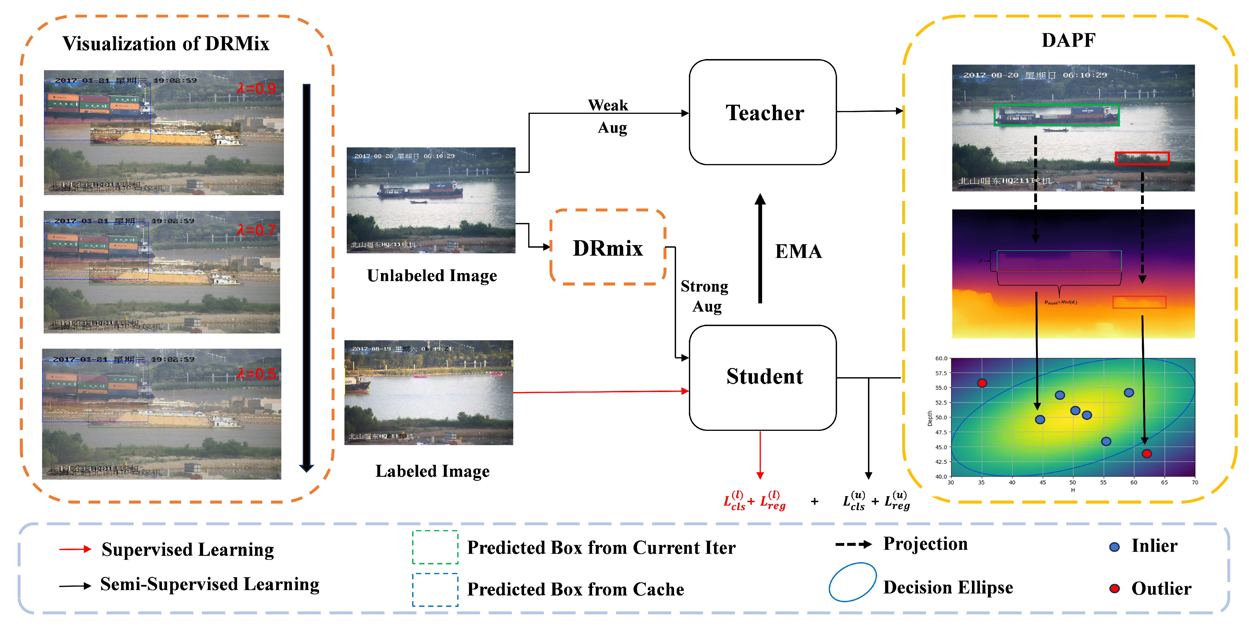
DAPF and DRMix. 

Table 3. Ablation results of the strategies in our model on the SeaShips dataset. DAPF denotes the depth-aware pseudo-label filtering strategy, and DRMix denotes the dynamic region mixup augmentation strategy.

DAPF	DRMix	AP50	AP50:95
		88.2	62.8
✓		91.0	66.0
	✓	89.9	65.0
✓	✓	92.0	66.2

presents different combinations with/without the two proposed strategies on the SeaShips dataset. The incorporation of depth-aware pseudo-label filtering (DAPF) resulted in remarkable increases of 2.8% in AP₅₀ and 3.2% in AP_50:95 over the baseline on the SeaShips dataset, thereby verifying its effectiveness. When replacing the mixup in Mixpl with our dynamic region mixup (DRMix) strategy, we observed performance increases of 1.7% in AP₅₀ and 2.2% in AP_50:95, indicating that our object-aware data augmentation strategy is better suited for object detection, especially in complex maritime scenarios. The full integration of both DAPF and DRMix yielded the best results, proving that the two components are complementary. Similarly, the same trends were also observed in the results on the SMD dataset, as shown in

Table 4. Ablation results of the strategies in our model on the SMD dataset.

DAPF	DRMix	AP50	AP50:95
		88.0	59.7
✓		88.7	60.6
	✓	88.3	60.1
✓	✓	89.1	60.9

, demonstrating both the effectiveness and generalization of our method across different datasets. To conclude, DAPF and DRMix are complementary and indispensable.

Besides the joint effect of DAPF and DRMix, we also examined the individual contribution of each component under different configurations on the SeaShips dataset.

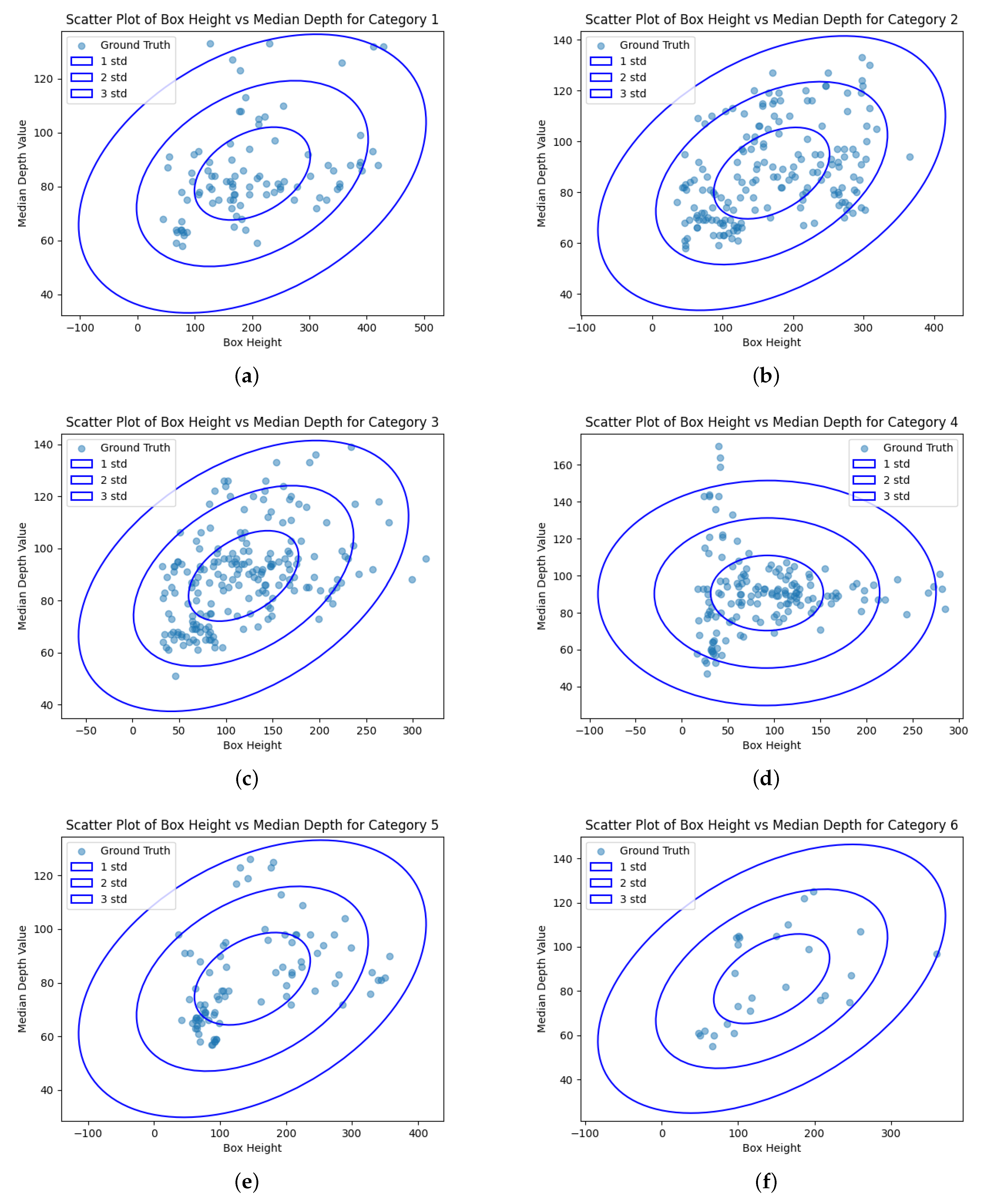
Analysis of DAPF. To further investigate DAPF, we conducted a quantitative analysis of its pseudo-label purification process in comparison to the baseline. As illustrated in Figure 6, which reports the number of false positives (FPs) and true positives (TPs) under varying classification confidence thresholds of the detector, DAPF significantly reduced the number of FPs by 36.5%, 16.9%, and 7.2% while retaining the majority of TPs. This indicates that DAPF can improve the quality of supervision, thereby contributing to enhanced detection performance.

We also performed an ablation study on the threshold parameter c using the SeaShips dataset, as shown in

Table 5. Performance under varying values of the threshold parameter c on the SeaShips dataset.

Threshold c	mAP
1	64.7
2	66.2
2.5	65.8
3	64.4

. Notably, an overly aggressive filtering threshold discarded valid pseudo-labels, resulting in degraded performance, which aligns with the observation shown in Figure 3. Empirical results indicate that setting c = 2 yields favorable performance, supporting the effectiveness of this choice.

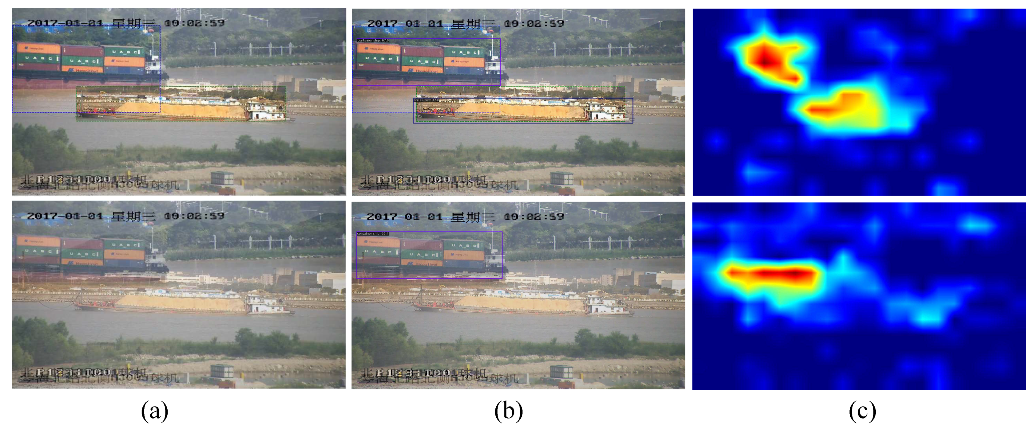
Analysis of DRMix. To examine the effect of DRMix, we employed Grad-CAM to visualize the results of the mixup technique in [16] and our DRMix technique. For a fair comparison, identical model weights were adopted for inference. As shown in Figure 7, DRMix effectively mitigated background interference with target object features by dynamically adjusting the mixing ratio between the target and background at the regional level. Consequently, DRMix produced a sharper and more focused heatmap that clearly highlights the relevant target regions. In contrast, the mixup strategy in [16] exhibited missed detection.

To further investigate the impact of the mixing ratio schedule, we conducted experiments comparing fixed and dynamic mixing ratio strategies during training, as summarized in

Table 6. Results of different mixing ratio ($\lambda$) schedules on the SeaShips dataset.

${\mathit{\lambda }}_{\mathbf{final}}$	${\mathit{\lambda }}_{\mathbf{init}}$	AP50:95
0.5	0.5	62.6
0.7	0.7	61.9
0.5	0.9	66.2

. The first two rows correspond to the degenerate and standard cases described in Equation (8), while the third row represents a curriculum-learning-inspired schedule. It is obvious that even a simple linear schedule exhibits clear advantages over fixed ratios.

Analysis of Labeled Data Sampling Ratio. To further verify the robustness and adaptability of our method under varying proportions of labeled data, we conducted experiments on the SeaShips and SMD datasets. Specifically, we assessed the model’s performance when trained with labeled data sampling ratios of 5%, 10%, 20%, and 50%. As shown in

Table 7. Experimental results with varying labeled data sampling ratios.

Dataset	Labeled Data Sampling Ratio	mAP	${\mathit{AP}}_{50}$	${\mathit{AP}}_{75}$
SeaShips	5%	56.8	85.0	65.0
	10%	66.2	92.0	80.6
	20%	68.8	93.4	83.0
	50%	72.3	94.9	84.1
SMD	5%	53.4	83.0	56.0
	10%	60.9	89.1	64.5
	20%	63.5	89.9	66.7
	50%	65.8	91.5	68.3

, on both datasets, the performance of the proposed model steadily improved as the proportion of labeled data increased, indicating that additional annotations facilitate the model’s generalization capability, as expected. Notably, even with only 5% of the labeled data, the model maintained relatively high accuracy, demonstrating its robustness under limited supervision.

5. Conclusions

In this paper, we aim to address the challenges of semi-supervised maritime object detection, an important yet under-explored domain. The scarcity of annotated maritime data weakens the direct application of SOTA terrestrial SSOD methods and even exacerbates error propagation. To tackle these issues, we propose two data-centric strategies. First, to enhance pseudo-label quality, we introduce the DAPF strategy, which leverages depth priors to effectively filter out unreliable pseudo-labels, thereby retaining more true positives while discarding false positives during training. Second, we present DRMix, a novel region-aware data augmentation technique with a dynamic training schedule tailored specifically for maritime object detection tasks. Extensive experiments on two maritime datasets demonstrate the effectiveness and superiority of the proposed algorithm. Furthermore, ablation studies validate the contribution and necessity of each component within the framework.

Despite our efforts in data engineering, several challenges remain for practical deployment. First, the current performance of the framework still falls short of industrial accuracy requirements. Second, the two datasets our method relies on lack sufficient samples of extreme or rare scenarios, such as heavy occlusions or severe weather conditions. The dynamic and complex nature of real-world maritime environments far exceeds the coverage of these datasets, which may lead to failures when encountering unseen situations. To solve these problems, future work will focus on integrating orthogonal advancements, such as the latest backbone architectures, into our pipeline to further boost performance. Additionally, collecting more diverse and challenging maritime datasets is critical to improve the generalization ability of SSOD models, both as training sources and as testbeds for long-term domain adaptation.