Experimental and Numerical Investigation of Localized Wind Effects from Terrain Variations at a Coastal Bridge Site

Abstract

Terrain conditions may significantly affect the near-ground-layer wind speed in coastal areas. In this research, wind tunnel tests and computational fluid dynamics (CFD) were performed to investigate the impact of topographic changes on the local wind field at coastal bridge sites. Considering the geographic information system (GIS) information of an offshore bridge site, a 1:1000 topographic model was constructed to conduct tests in the wind tunnel lab under different wind directions. The influences of terrain conditions on localized wind characteristics such as the wind speed and wind attack angle under different test conditions were obtained. The results show that the wind angle varied between −6° and 6° under different conditions. To more comprehensively show the radius of influence on the local terrain, a CFD simulation was conducted. To verify the results of the wind tunnel tests, the SST k-ω model was compared and selected for simulation in this research. The influence radius of localized wind characteristics was determined by CFD simulation. The results indicate that the original topography showed “reverse amplification” on the leeward side, resulting in complex wake flows. These results may provide a reference for the design of wind-resistant structures such as bridges and offshore wind turbines in coastal areas.

1. Introduction

With the ongoing expansion of infrastructure development in coastal regions, particularly the construction of long-span bridges, wind resistance has emerged as a pivotal concern in both design and research [1,2]. The intricate terrain and frequent high-wind conditions, such as typhoons, prevalent in coastal areas profoundly influence the wind load characteristics of bridges, thereby impacting their wind resistance and structural integrity [3,4]. Within this framework, bridge structures, characterized by their extensive spans and relatively low stiffness, exhibit heightened sensitivity to wind forces [5]. This sensitivity is exacerbated when significant local topographic variations occur, as they introduce greater complexity to the wind field, potentially triggering phenomena such as wind speed amplification and flow separation near the bridge site, which pose fresh challenges to wind-resistant design. Consequently, investigating the local wind effects induced by topographic changes is of substantial practical importance for enhancing the wind resistance design of bridges.

Methods for examining local wind effects in bridge site areas primarily include field measurements, experimental studies, and numerical simulations. Field measurements deliver authentic wind field data by using wind speed measurement devices such as Windcube (Leosphere., Orsay., Ile-de-France., France) or wind observation towers for data acquisition and analysis [6,7,8,9,10]. For example, Wang et al. [4] assessed the wind field characteristics of the Sutong Bridge region through prolonged monitoring, whereas Hui et al. [11] analyzed the wind field properties of Hong Kong’s Shek Mun Bridge via field measurements, revealing substantial variations in turbulence characteristics between the open sea and terrestrial environments; however, field measurements frequently encounter obstacles such as extended timeframes, high expenses, and limitations posed by outdoor environmental conditions.

Compared with field measurements, wind tunnel experiments are unaffected by outdoor environmental constraints and entail reduced labor costs, effectively reproducing the wind field characteristics of complex terrains using scaled models [12,13,14,15,16]. In bridge design for flat regions, where terrain exerts minimal influence on incoming flow, wind field parameters such as the wind speed and angle of attack typically display uniform variation along the bridge span [17]. In contrast, under complex terrain conditions such as coastal and mountainous regions, the wind speed and angle of attack exhibit significant fluctuations due to local topographic features, such as shielding effects and ridge effects, which profoundly shape the distribution of the local wind field [18,19,20]. Through wind tunnel testing, Chen et al. [21] explored the wind characteristics in mountainous areas and observed substantial acceleration of the wind speed at mountaintops and mountain passes, whereas deceleration at the foothills was attributable to shielding effects. Additionally, wind direction plays a pivotal role in determining wind field characteristics. Yan et al. [22] examined the wind field properties at bridge sites in southeastern Tibet’s mountainous region and reported that the wind speed and turbulence intensity are influenced not only by the wind direction but also by the measurement location, with a particularly pronounced increase in the wind speed when airflow descends from mountaintops. Similarly, Li et al. [23] utilized wind tunnel experiments to investigate the wind field characteristics of bridges in mountainous terrain, identifying a distinct acceleration in the wind speed in the leeward region as airflow passes over a ridge.

With the rapid advancement of computational fluid dynamics (CFD) technology, a growing number of studies have harnessed CFD to simulate local wind effects in complex terrains, highlighting its high accuracy and robust operability in capturing terrain-induced phenomena such as wind field acceleration, sheltering, and flow separation [24,25,26,27,28]. Nabil et al. [29] employed numerical simulations to analyze airflow over a prominent peak on a steep mountainside and its effects on a scenic platform. Using CFD simulations, Song et al. [30] investigated the impact of converging river channel terrain on the wind characteristics of the Yellow River Bridge. Hu et al. [31] utilized the SST k-ω model to examine the wind speed and turbulence intensity across a simplified canyon terrain, confirming the model’s efficacy. Concurrently, ensuring the accuracy of simulation results has underscored equilibrium atmospheric boundary layer (ABL) self-sustainability as a critical factor necessitating meticulous attention in CFD analyses. To this end, the challenge of maintaining the self-sustainability of the ABL in CFD simulations has attracted considerable attention, with studies by Yang et al. [32,33] highlighting the pivotal role of ABL models in achieving dependable simulation outcomes.

Although numerous studies have investigated the effects of local wind under complex terrain conditions, accurately assessing the impact of local terrain changes on the wind field at bridge sites in the context of large-scale terrain modifications remains an unresolved challenge. This study focused on a bridge site along the southeastern coast as the research subject. By integrating the requirements of the equilibrium atmospheric boundary layer (ABL), a combined approach of computational fluid dynamics (CFD) numerical simulation and wind tunnel testing was employed to investigate the wind field characteristics under the original terrain scenario and a modified terrain scenario (with a portion of the mountain removed). Figure 1 shows the geographical situation of the bridge site before and after the terrain modification, where the red line represents the modified terrain area, and the yellow line indicates the bridge site area. It can be seen that the terrain features changed significantly after the mountain was excavated. The analysis emphasized key parameters at the main deck height of the bridge site under different wind directions, including the wind speed, angle of attack, mean wind profile, and local wind effects induced by the terrain. Furthermore, by comparing the results of the numerical simulations with those of the wind tunnel experiments, the differences in the wind field distributions between the two terrain scenarios and their underlying causes are elucidated.

While this study primarily investigates the localized wind effects caused by terrain variations in the case of boundary layer wind, it is well known that the effect of terrain also becomes significant in the presence of high-intensity winds, such as those associated with typhoons or other extreme weather events. These high-intensity winds can further accentuate the disturbances in the wind field caused by terrain features, leading to greater challenges in wind-resistant design, especially for large infrastructure projects like bridges. Therefore, while the current study focuses on boundary layer winds, the potential for more pronounced effects in high-intensity winds highlights the importance of considering such scenarios in future investigations.

2. Wind Tunnel Experimental

2.1. Geographic Information

This study focused on a proposed bridge site along China’s southeast coast, featuring a span arrangement of 24 × 30 m + 2 × 240 m + 22 × 30 m and a 480 m main span configured as a single-tower cable-stayed bridge (Figure 2a). The terrain enveloping the bridge site stretches east–west, bordering a mountain approximately 100 m in elevation to the south and a northern mountain range that impedes incoming wind, with a river coursing from west to east across the site (Figure 2b). To assess the effects of topographic alterations on the wind field, this study performed a comparative analysis through numerical simulations and wind tunnel experiments under two scenarios: the original terrain scenario (with the mountain intact) and a modified terrain scenario (with a portion of the mountain removed). The experimental design integrated diverse incoming flow conditions and monitoring point layouts (Figure 2a,c).

Table 1. Experimental and simulation cases.

Case	Contrast/Original Terrain (A/B)	Bridge Span Location
Case 1	without/with mountains	starting point, 4/L, 2/L, 3/4L, finishing point
Case 2	without/with mountains	starting point, 4/L, 2/L, 3/4L, finishing point
Case 3	without/with mountains	starting point, 4/L, 2/L, 3/4L, finishing point
Case 4	without/with mountains	starting point, 4/L, 2/L, 3/4L, finishing point
Case 5	without/with mountains	starting point, 4/L, 2/L, 3/4L, finishing point
Case 6	without/with mountains	starting point, 4/L, 2/L, 3/4L, finishing point

specifies the experimental and simulation scenarios, with Condition A representing the modified terrain and Condition B indicating the original terrain, encompassing 12 cases across 6 incoming wind directions (e.g., Case 1(A) and Case 1(B)).

2.2. Wind Tunnel Experimental Setup

The experiments for this study were performed at the XMUT-WT wind tunnel laboratory at Xiamen University of Technology. The wind tunnel lab contains a high-speed section (8 m × 2.6 m × 2.8 m, with an adjustable wind speed range of 2~85 m/s) and a low-speed section (25 m × 6 m × 3.6 m, with an adjustable wind speed range of 0.5~3 m/s). To fit the test size in the low-speed section, a terrain model was constructed at a 1:1000 scale, featuring a diameter of approximately 5 m and a maximum height of approximately 0.2 m, centered on the sea level near the bridge site. The ratio of the model’s cross-sectional area to that of the wind tunnel was calculated to be approximately 1.11%, which is much lower than the recommended blockage threshold of 5%.

To examine the influence of local topographic variations on the wind field at the bridge site, wind tunnel tests were performed on two models: the original terrain scenario and the modified terrain scenario (with a portion of the mountain removed) (see Figure 3). In the experiments, wind speed measurements were conducted using Cobra probes manufactured by Turbulent Flow, with a measurement range of 2–200 m/s and an accuracy of ±0.5 m/s. Prior to the experiments, all Cobra probes were calibrated according to standard procedures to ensure data reliability. Fourteen monitoring points were positioned across a height range of 0.35 m, arranged along the bridge span (at the starting point, L/4, L/2, 3L/4, and the ending point). Wind speed data were collected at a sampling frequency of 1000 Hz and recorded through a data acquisition system, with each data collection lasting 60 s to obtain stable average wind speed and turbulence characteristics. To simulate natural wind characteristics, the incoming wind speed and turbulence intensity were adjusted using roughness elements and spires to meet the Class A wind field characteristics (see Figure 4) [34]. The roughness elements consisted of cubic blocks with a height of 0.04 m, uniformly distributed at the wind tunnel entrance, and the spires were approximately 2 m in height with a base width of 0.35 m, ensuring that the wind speed profile and turbulence intensity conformed to the specified requirements.

3. Numerical Methods

3.1. Turbulence Model

In numerical simulations over complex terrains, the Reynolds-Averaged Navier–Stokes (RANS) method offers greater computational efficiency than does large eddy simulation (LES) while still capturing wind field characteristics with sufficient accuracy for engineering applications. Notably, the shear stress transport SST k-ω model combines the advantages of the k-ε and k-ω models, enabling precise simulation of turbulence in the near-wall region and effective handling of free shear flow zones. Previous research has shown that this model achieves strong agreement with wind tunnel data in wind field simulations at bridge sites, accurately reflecting real-world flow characteristics. Consequently, this study adopted the SST k-ω model for its numerical simulations. The transport equations of the SST k-ω model are as follows:

$${\displaystyle \frac{\partial \left(\rho k\right)}{\partial \left(t\right)}}+{\displaystyle \frac{\partial \left(\rho k{u}_i\right)}{\partial \left(x_i\right)}}={\displaystyle \frac{\partial }{\partial \left(x_i\right)}}\left[\left(\mu +{\displaystyle \frac{{\mu }_t}{{\sigma }_k}}\right){\displaystyle \frac{\partial k}{\partial x_i}}\right]+\overline{G_k}-Y_k+S_k$$

(1)

$${\displaystyle \frac{\partial \left(\rho \omega \right)}{\partial \left(t\right)}}+{\displaystyle \frac{\partial \left(\rho \omega u_i\right)}{\partial \left(x_i\right)}}={\displaystyle \frac{\partial }{\partial \left(x_i\right)}}\left[\left(\mu +{\displaystyle \frac{{\mu }_t}{{\sigma }_{\omega }}}\right){\displaystyle \frac{\partial \omega }{\partial x_i}}\right]+\overline{G_{\omega }}-Y_{\omega }+D_{\omega }+S_{\omega }$$

(2)

where $\overline{G_k}$ is the production term of the turbulent kinetic energy (TKE) induced by the mean velocity gradient; $\overline{G_{\omega }}$ is the production term of the dissipation rate; $Y_k$ and $Y_{\omega }$ represent the dissipation terms associated with the turbulence-induced TKE and dissipation rate, respectively; $D_{\omega }$ denotes the cross-diffusion term; $S_k$ and $S_{\omega }$ are user-defined source terms; and ${\sigma }_k$ and ${\sigma }_{\omega }$ are the respective Prandtl numbers for the TKE and dissipation rate.

3.2. Numerical Model

Using the sea level center near the bridge site as the reference point, a terrain model of the bridge site was constructed with a radius of approximately 2.5 km. A scale of 1:1000 was selected on the basis of the actual elevation and the dimensions of the wind tunnel. The northern side of the model corresponds to a region of higher elevation in the real terrain. To ensure a smooth transition in the terrain, a sloping transition section was incorporated into the northern part, where significant topographic variations are present. The computational domain was configured with a “velocity inlet” at the entrance and a “pressure outlet” at the exit, while the top, bottom, and lateral boundaries were designated symmetry boundaries. Consistent with the wind tunnel configuration, the horizontal distance from the model center to the wall was approximately 3 m, with the inlet and outlet widths set at 18 m and 7 m, respectively. The incoming flow was characterized by a power-law wind profile, with the inlet wind speed distribution defined as follows:

$$\begin{gathered} V(z)=V_{0.22}{\left({\displaystyle \frac{z}{0.22}}\right)}^{\alpha },0\le z\le 0.3\mathrm{m} \\ V(z)=V_{ref},z>0.3\mathrm{m} \end{gathered}$$

(3)

where z is the vertical distance between the measurement point and the ground; α is the power-law exponent, which was set to 0.12 for A-type terrain; $V\left(z\right)$ is the wind speed at height z; $V_{0.22}$ is the basic wind speed at z = 0.22 m, which was obtained via least-squares fitting; and $V_{ref}$ = V_0.3 is the reference wind speed at z = 0.3 m.

To examine the influence of local terrain variations on the wind environment in the bridge site area, numerical simulations were conducted for two terrain scenarios: the original terrain and a modified terrain scenario (with a portion of the mountain removed). Furthermore, validations were carried out to evaluate grid independence and the self-preserving properties of the equilibrium atmospheric boundary layer (ABL).

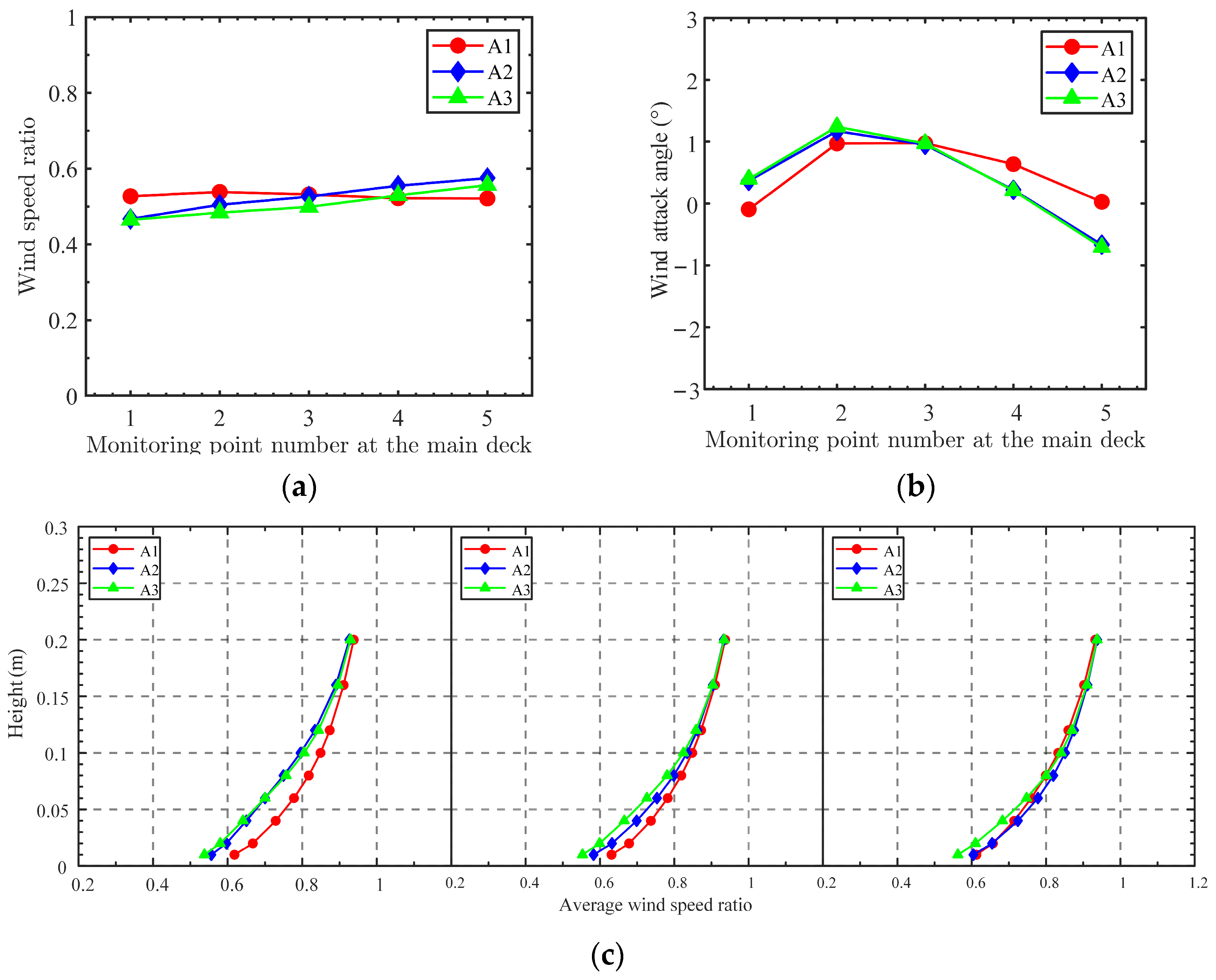
3.3. Terrain Model Meshing

To ensure the accuracy of the terrain model’s grid partitioning and to obtain reliable simulation results, a grid independence test was initially performed. A prismatic grid was utilized within the terrain region, whereas a hexahedral grid was applied to the remainder of the computational domain. Figure 5 depicts the near-wall grid configuration, and

Table 2. Detailed mesh configurations of three terrain models under comparative terrain conditions.

Mesh	Min. Grid Size on Terrain (m)	Min. Grid Size (m)	First-Layer Boundary Height (m)	Growth Rate	Total Cells
A1	0.03	0.1	0.0009	1.13	1,549,914
A2	0.02	0.05	0.0007	1.13	3,202,482
A3	0.01	0.04	0.0003	1.13	6,579,340

presents the key parameters of the three grid schemes employed for the grid independence validation.

For the numerical simulation, the SST k-ω turbulence model was utilized. A fully implicit, three-dimensional, double-precision segregated solver was employed, with velocity–pressure coupling achieved through the SIMPLEC algorithm. The convection terms were discretized using a second-order upwind scheme. A transient analysis was conducted with a time step of 0.01 s. The transverse wind velocity and angle of attack at the main deck height, along with the mean wind velocity profiles at the starting point, L/4, and L/2 positions within the terrain variation zone, were monitored primarily to assess the mesh independence and simulation accuracy.

Using the Case 1 modified terrain scenario as an example, Figure 6 displays the transverse wind speed at the main deck height, the angle of attack, and the mean wind speed profiles at the starting point, L/4, and L/2 positions for the A1, A2, and A3 grid configurations. The results reveal that, in Figure 6a, the difference in transverse wind speed between grids A2 and A3 was negligible (with a relative error of approximately 3.69%), whereas A1 had a larger error (approximately 7.78%); the angle of attack in Figure 6b had a similar trend; in Figure 6c, A1 had a relative error as high as 8.28% near the start of the mountain region, whereas A2 had an error of only 1.34%. To balance accuracy and computational efficiency, the A2 grid configuration was deemed preferable.

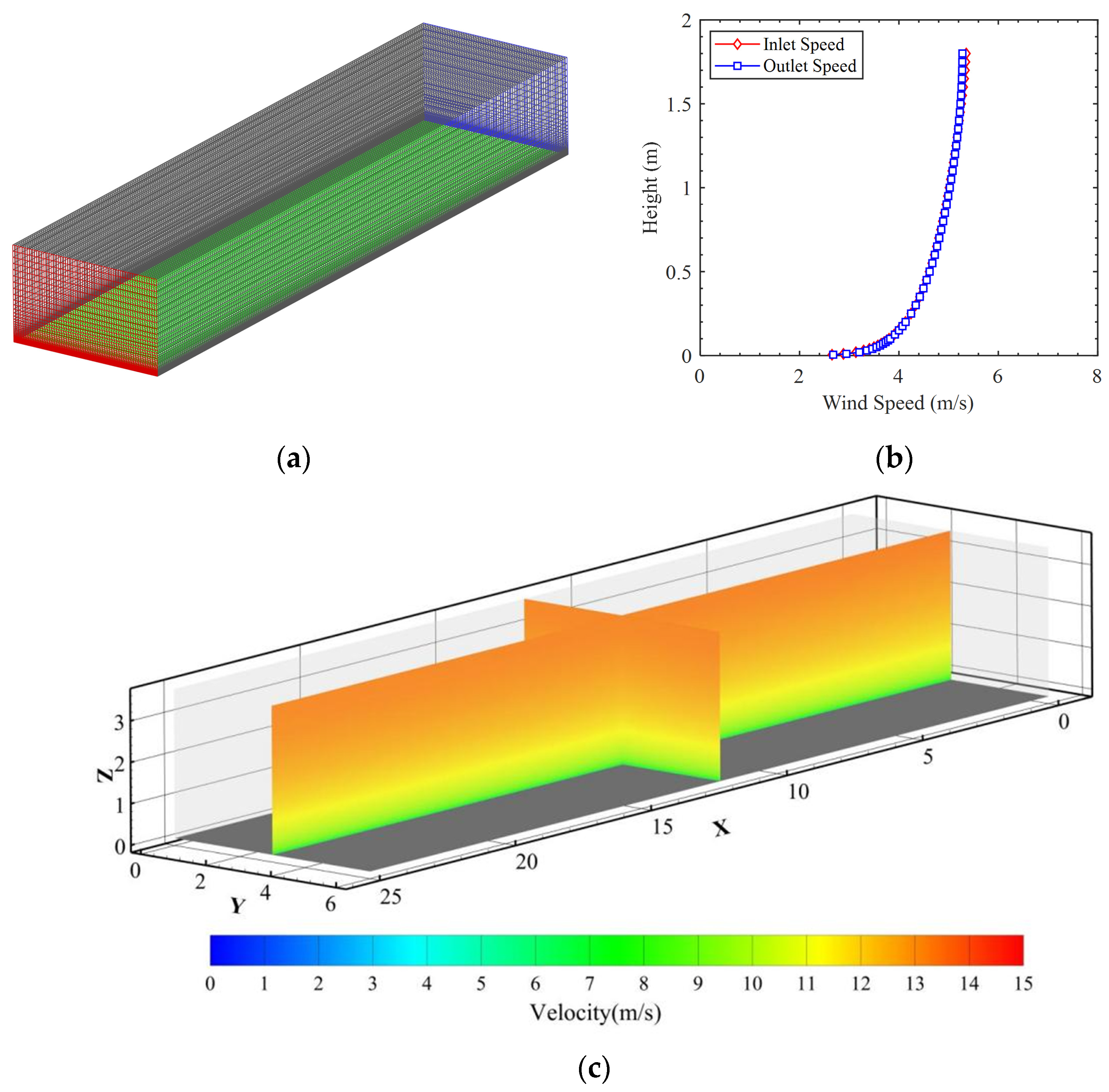
3.4. Equilibrium Atmospheric Boundary Layer (ABL) Analysis

To ensure the accuracy of the simulated inlet wind velocity profile, validation of the equilibrium atmospheric boundary layer (ABL) was also necessary. The formula proposed by [33], which is based on the SST k-ω turbulence model, was adopted as a reference:

$$V=V_{ref}{\left({\displaystyle \frac{z}{z_{ref}}}\right)}^{\alpha }$$

(4)

$$k=\sqrt{D_1{z}^{\alpha }+D_2}$$

(5)

$$\omega ={\displaystyle \frac{\alpha }{\sqrt{C_{\mu }}}}{\displaystyle \frac{V}{z}}$$

(6)

In the equation, $V_{ref}$ and $z_{ref}$ represent the reference wind speed and reference height, which were obtained by fitting the experimental inlet wind profile; $\alpha$, corresponding to an A-type wind field, was set to 0.12; $k$ denotes the turbulent kinetic energy; $D_1$ and $D_2$ are undetermined constants characterizing the inlet turbulence, determined by fitting wind tunnel data; and ω is the specific dissipation rate, with $C_{\mu }$ set to 0.028. Figure 7a,b present the fitting results for the velocity and turbulent kinetic energy, respectively.

A computational domain corresponding to the wind tunnel dimensions (25 m × 6 m × 3.6 m) was constructed, with the first-layer grid height set at 0.00045 m, a growth rate of 1.13, and horizontal and transverse grid spacings of 0.1 m; all other parameters remained consistent with the previously specified settings. The numerical results demonstrate that, in addition to minor deviations near the top and ground at the inlet and outlet, the flow velocity distribution in the remaining regions closely aligns with the inlet profile, with a maximum relative error of approximately 2.23%. Velocity cloud maps (see Figure 8) indicate that the incoming flow was well maintained throughout the computational domain, confirming that the inlet turbulence boundary conditions fulfilled the requirements of the equilibrium atmospheric boundary layer (ABL), thereby providing reliable assurance for subsequent simulations.

4. Results and Discussion

To assess the impact of local terrain variations on the wind field at the bridge site, transverse wind velocities and angles of attack at the main deck height, along with mean wind velocity profiles at the starting point, L/4, and L/2 positions near the mountain side, were derived from both numerical simulations and wind tunnel experiments. A comparative analysis of local wind effects was conducted between the original terrain scenario and the modified terrain scenario (with a portion of the mountain removed). In this study, the positive transverse wind direction was defined as west to east, and the positive angle of attack was defined as upward from the underside to the top of the main deck. To facilitate comparison, the following normalized definitions of the wind velocity and angle of attack were introduced:

$${\overline{V}}_H={\displaystyle \frac{V_H}{V_{ref}}}$$

(7)

$$\theta ={tan}^{-1}\left({\displaystyle \frac{V_V}{V_H}}\right)$$

(8)

In this context, ${\overline{V}}_H$ denotes the dimensionless wind speed, $V_H$ represents the cross-bridge wind speed, $V_{ref}$ represents the gradient wind speed at the inflow boundary, $V_V$ represents the vertical main deck wind speed, and $\theta$ represents the angle of attack at the main deck height.

4.1. Transverse Wind Velocity at the Main Deck Height

Figure 9 presents comparisons between the numerical simulation (CFD) and wind tunnel measurements of the dimensionless transverse wind velocity at the main deck height under different inflow conditions. Measuring point 1 is closest to the terrain variation zone, with higher measuring point numbers indicating increased distance from this zone.

As depicted in Figure 9a (Case 1, 45°), a local low-velocity zone emerged near the mountainside under the original terrain scenario, with wind speeds approximately 12% lower than those observed under the modified terrain scenario; the numerical simulation results reveal an even more pronounced difference, reaching up to 25%. This discrepancy gradually decreased with increasing distance from the terrain variation zone. Under the modified terrain scenario (with a portion of the mountain removed), the previously obstructed low-speed zone vanished, leading to a substantial increase in the wind velocity on this side. Both the numerical and experimental results confirm that mountainous terrain had a distinct “suppression-recovery” effect on local wind velocities.

In Figure 9b,e (Case 2 and Case 5, 90° and 270°, respectively), the incoming flow was predominantly governed by sea surface winds, with wind directions approximately perpendicular to the bridge site, leading to reduced terrain-induced disturbances. Under both the original and modified terrain scenarios, the transverse wind velocity distributions at the main deck height remained relatively consistent. Compared with other cases, the variations between measuring points were minimal, typically within 3%.

Figure 9c,f (Case 3 and Case 6, 135° and 315°, respectively) illustrate that, under the original terrain scenario, local acceleration occurs near the mountain side due to terrain protrusion, yielding wind speeds approximately 10% higher than those observed under the modified terrain scenario. Under the modified terrain scenario (with a portion of the mountain removed), this acceleration effect vanished, and the wind velocity became relatively consistent, resulting in a corresponding decrease in the wind speed on this side.

The results from Figure 9d (Case 4, 225°) suggest that, compared with the original terrain scenario, the modified terrain scenario (with a portion of the mountain removed) had a relatively modest effect on the wind velocity along the bridge axis. Nonetheless, the overall wind velocity generally remained elevated, with this effect being particularly pronounced near the terrain variation zone.

Additionally, as illustrated by the velocity cloud maps in Figure 10, pronounced flow separation and vortex shedding phenomena were observed in Case 1 (45°) under the original terrain scenario, leading to a distinct low-velocity zone near the mountain side. Under the modified terrain scenario, the wind speed at the main girder in this region increased by approximately 25%. Conversely, Case 6 (315°) displayed contrasting behavior: the original terrain scenario triggered local acceleration due to terrain protrusion, whereas the modified terrain scenario resulted in a more uniform wind velocity distribution and reduced overall fluctuations. For scenarios such as Case 2 (90°), where the wind predominantly originates from the sea surface, wind velocity variations remained minimal, and the impact of terrain modifications was consequently diminished.

In summary, the influence of local terrain variations on the transverse wind velocity at the main deck height exhibited a distinct dependency on the wind direction: when the incoming flow forms an angle with the mountain orientation, the effects of blockage, flow separation, and acceleration become more pronounced at the bridge site; however, when the flow is perpendicular to the mountain alignment, local disturbances at the bridge site are relatively minor. Overlooking the wind field variations caused by terrain changes in engineering design may lead to an underestimation of actual wind loads, thereby affecting both the safety and economic efficiency of the bridge’s wind-resistant design.

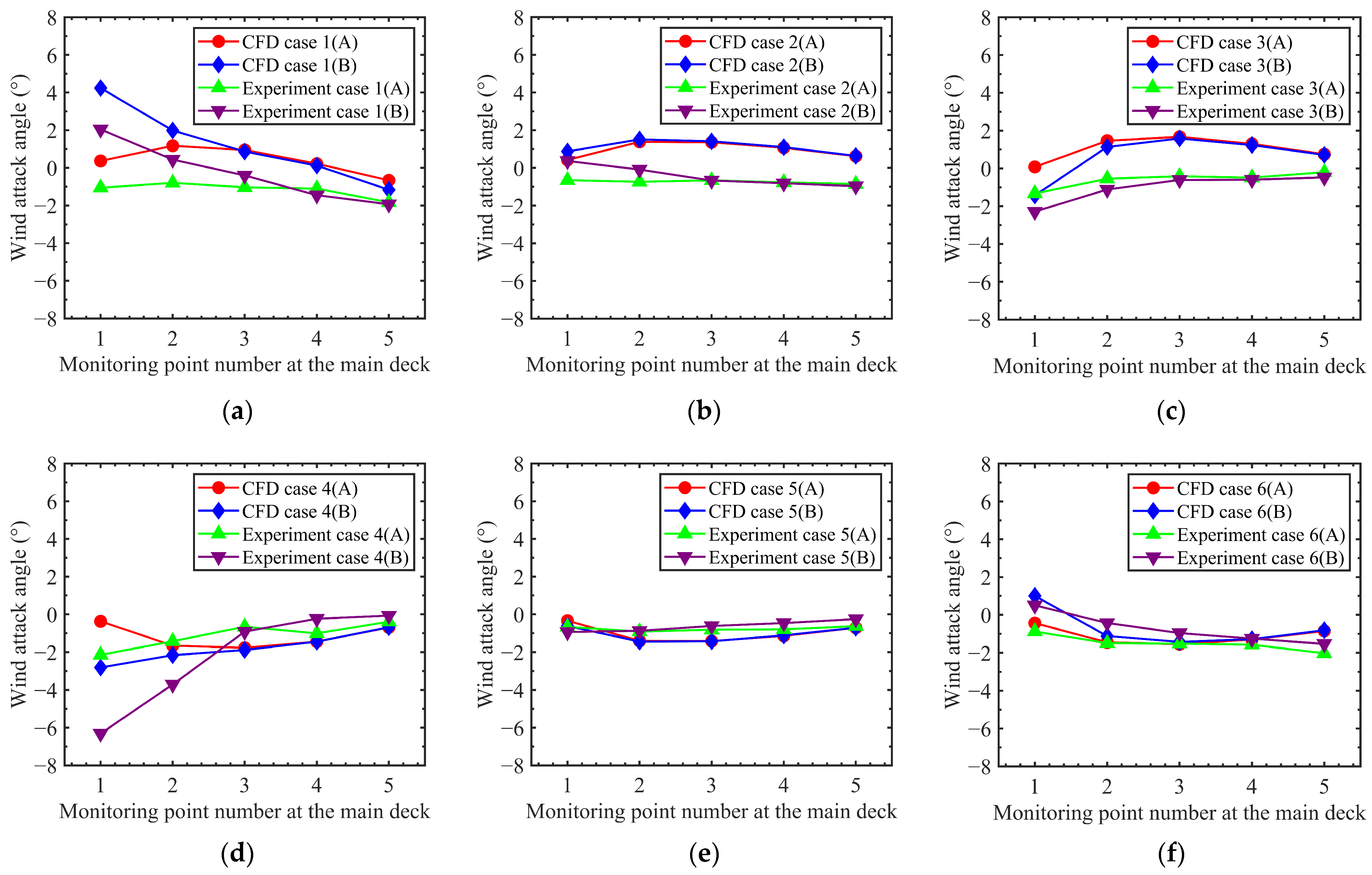
4.2. Angle of Attack at the Main Girder Level

Figure 11 shows the variations in the angle of attack at the main deck height under the original and modified terrain scenarios across different wind directions. Under the original terrain scenario, the angle of attack exhibited greater fluctuations (e.g., experimental results reached up to 2° in Case 1, with numerical simulations peaking at 5°), whereas these fluctuations were significantly reduced under the modified terrain scenarios, occasionally shifting from positive to negative values (experimental results decreased to approximately −2°, with simulations at approximately −1°). A similar pattern emerged in Case 4: the original terrain scenario displayed a broader range of angles of attack (experimentally spanning −6° to 0°), which narrowed to between −3° and −1° under the modified terrain scenario. This suggests that terrain modification, such as the partial removal of mountain features, can effectively mitigate fluctuations in the amplitude of the angle of attack.

Figure 11b,e illustrate that for Cases 2 and 5 (90° and 270°, respectively), the overall variation in the angle of attack remained relatively small, generally confined to a range of −2° to 2°. The influence of the two terrain scenarios on the angle of attack showed no substantial difference, suggesting that under this perpendicular inflow scenario, the mountain’s interference with the wind field at the bridge site was comparatively minor.

Figure 11c,f reveal that terrain variations exerted a more pronounced influence on the angle of attack at the main deck height for Cases 3 and 6 (135° and 315°, respectively). In Case 3, under the original terrain scenario, the angle of attack spanned approximately −3° to −1° (with numerical simulations ranging from −2° to 1°), whereas under the modified terrain scenario, this range contracted to −1° to 0°, suggesting that the original terrain was more prone to inducing local flow instability. Similarly, the experimental results from Case 6 indicate that the modified terrain scenario reduced the angle of attack range from approximately 1° to −2° to approximately −1° to −2°, mitigating the effects of local acceleration or flow separation.

Overall, both the numerical simulations and the wind tunnel experiments suggest that the original terrain scenario generally produced greater fluctuations in the angle of attack at the main deck height, with the test and simulation results showing the maximum range of the angle of attack between −6° and 6°. In contrast, the modified terrain scenario led to more stable angles, with the maximum range of the angle of attack between −2° and 2°. As the distance from the terrain variation zone increased, the terrain-induced effects progressively diminished.

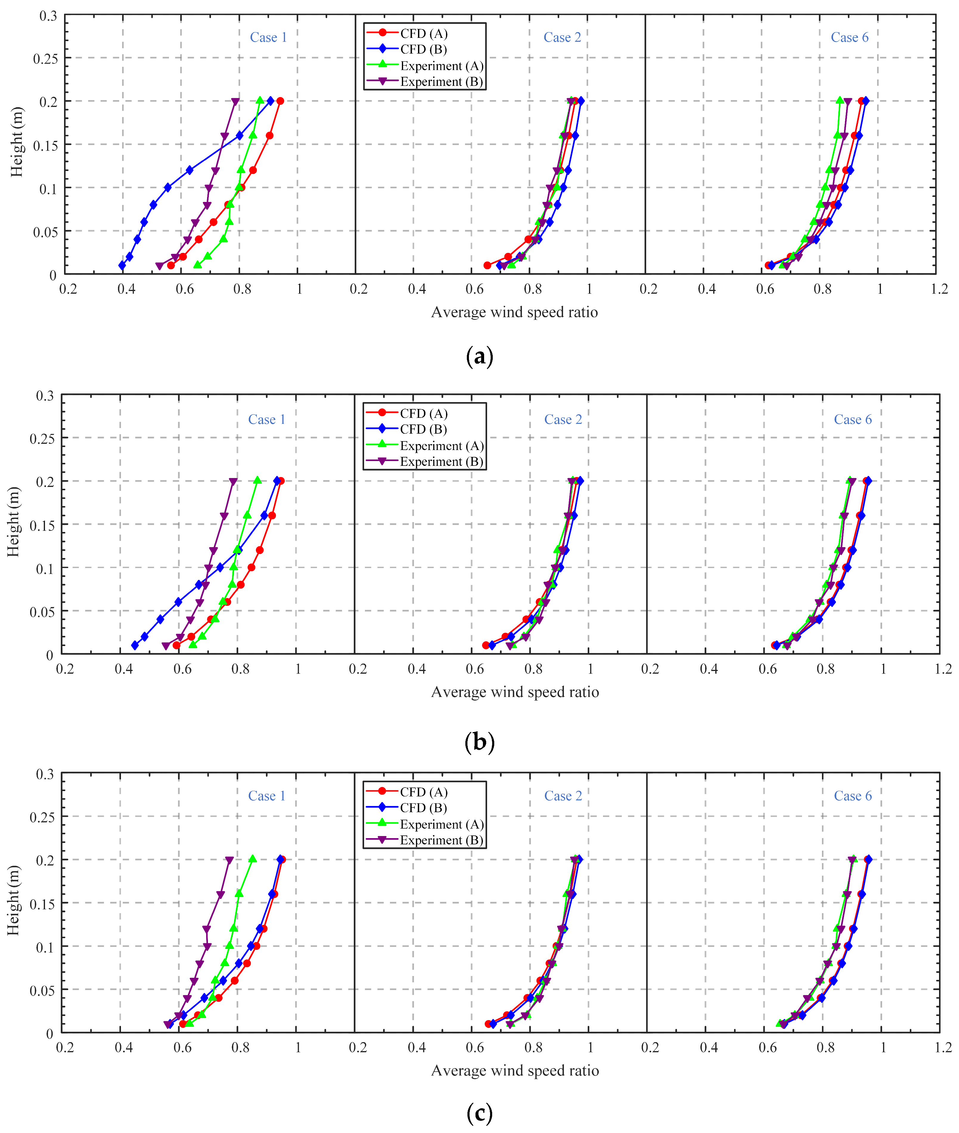
4.3. Mean Wind Profiles

The mean wind speed ratio was defined as the ratio of the measured (or simulated) mean wind speed at the bridge site to the inlet gradient wind speed. On the basis of the preceding analysis, the mean wind speed ratio profiles at three monitoring points—the bridge starting point, L/4, and L/2—under typical wind directions were selected for both the original and modified terrain conditions, as shown in Figure 12. Overall, the wind speed ratio increased with height at all locations, but the differences were more pronounced in areas closer to the terrain modification zone.

As shown in Figure 12a, for Case 1 (45°), the mean wind speed ratio under the original terrain condition was significantly lower than that under the modified terrain condition, with a difference of up to 20% near the ground (reaching 30% in simulations), primarily due to the blocking effect of the mountain. As the height increased, the two conditions gradually converged. For the other cases (Cases 2 and 6), the differences in the wind speed ratio were smaller, with overall variations of approximately 5%.

As the monitoring points were farther from the modified mountain terrain (Figure 12b), the wind speed ratio discrepancy for Case 1 diminished. With increasing height, the trends gradually converged. For other wind directions, terrain-induced disturbances were further attenuated, resulting in relatively stable wind speed ratio profiles with height, and the impact of terrain modification on the wind speed ratio was minimal.

At the L/2 position of the bridge, the differences were further reduced. Particularly when the incoming flow was nearly perpendicular to the bridge alignment (e.g., Case 2), the wind speed ratios under the two terrain conditions were essentially identical, indicating that local terrain changes have a limited impact on the wind field in more distant regions.

A comprehensive analysis of Figure 12 revealed that the starting point (Case 1) was most significantly affected by local terrain changes, with the near-ground wind speed ratio under the modified terrain condition increasing by approximately 20% (and up to 30% in simulations). This influence gradually weakened as the distance extended to L/4 and L/2, eventually converging. For cases with inherently uniform incoming flow (e.g., Case 2), the blocking effect of the mountain under the original terrain condition had a more limited impact on the bridge site, and the wind speed ratio variations between the two terrain conditions remained relatively stable.

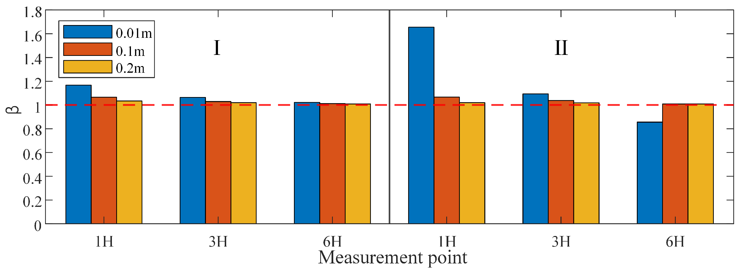
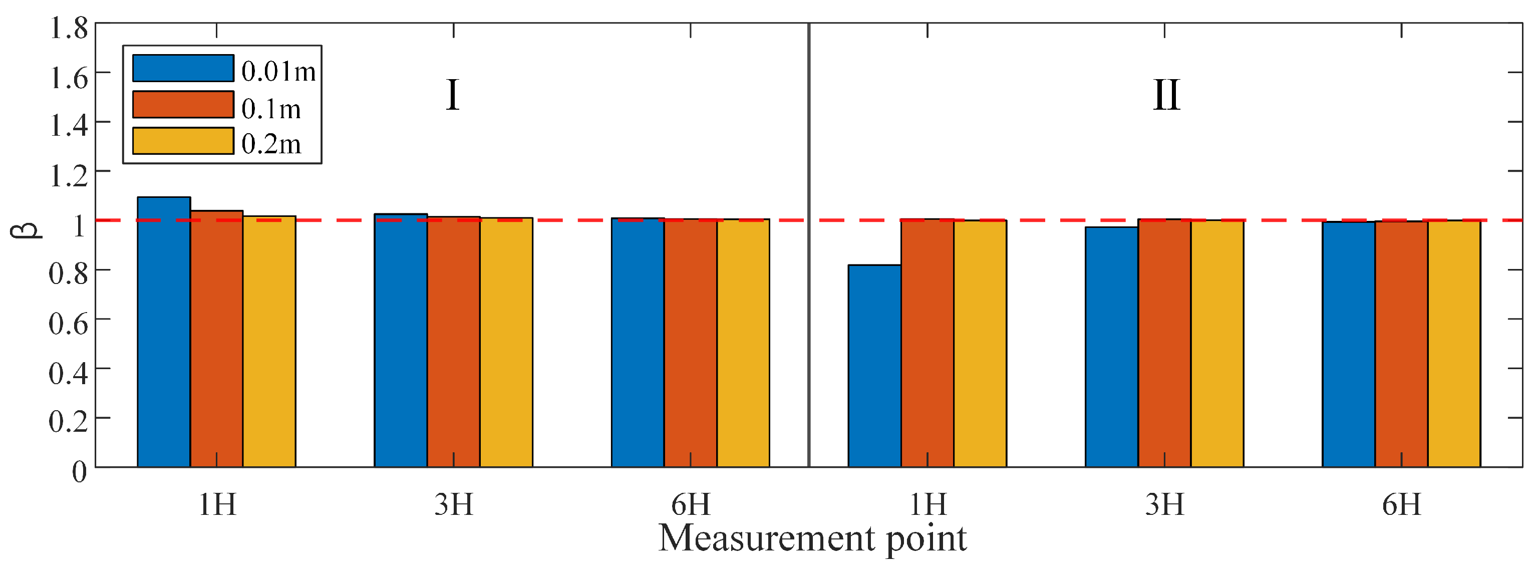
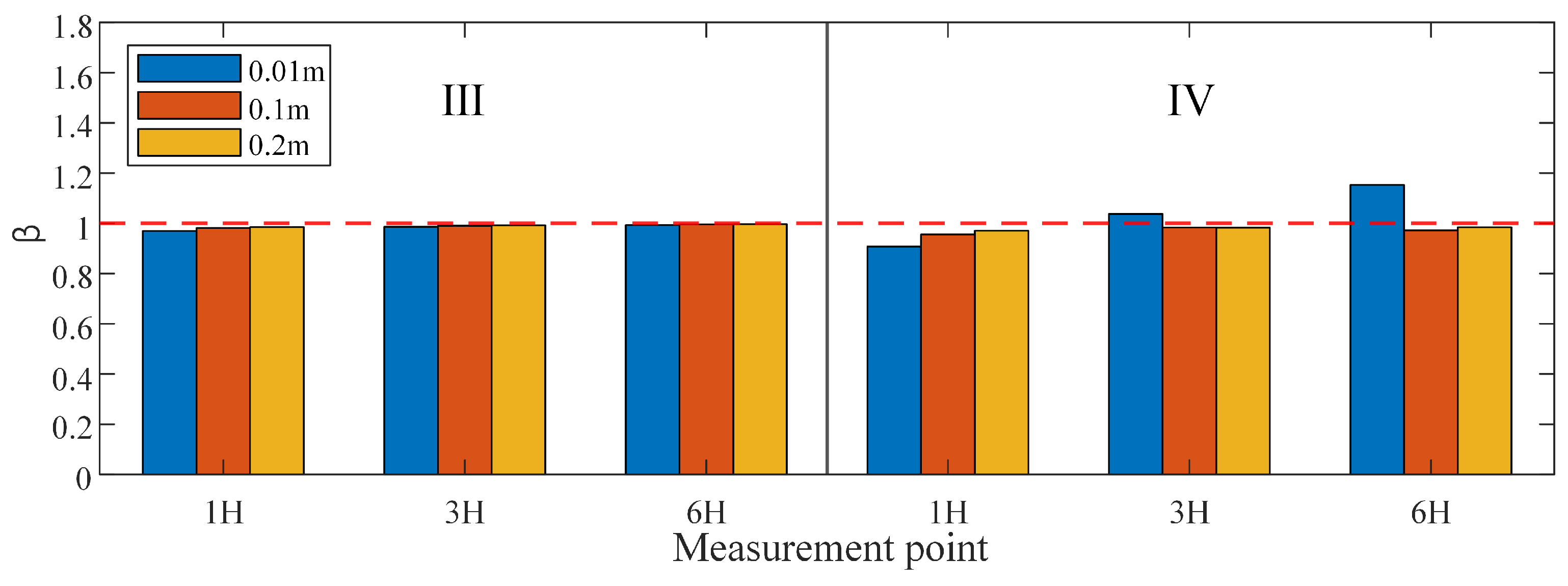
4.4. Error Analysis of the Experimental and Numerical Results

Figure 13 and Figure 14 present a point-by-point comparison of the mean wind speed ratio and wind attack angle at various monitoring points under the two terrain conditions. The results indicate that under the original terrain conditions, the scatter distribution was more dispersed. At the section closest to the mountain, the relative error in the wind speed reached approximately 30%, and the maximum deviation in the wind attack angle approached 50%. This reflects the limitations of the numerical model in fully capturing the shielding, shear, and separation effects induced by complex terrain. As the monitoring points were farther from the terrain variation zone, the errors rapidly converged, suggesting that the overall trends were still accurately reproduced.

In contrast, when the terrain was leveled or smoothed, the uniformity of the incoming flow improved significantly, and the discrepancies between the numerical and experimental results decreased correspondingly. As shown in the figures, under the modified terrain condition, all the wind speed measurements were within a ±10% error range, with 80% of the data points falling within this interval. A similar trend was observed for the wind attack angle. The scatter points clustered closer to the diagonal, indicating a more concentrated distribution and demonstrating that the reliability of CFD predictions for velocity fields and flow directions is substantially enhanced when terrain irregularities are reduced.

Collectively, the figures reveal that the nonuniformity of the flow field caused by the original terrain is the primary source of error. Once terrain irregularities are mitigated, local disturbances diminish, leading to reduced errors. These findings underscore the importance of detailed modeling of complex terrain features in the assessment of wind environments and the design of wind-resistant structures at bridge sites. Furthermore, if engineering plans involve terrain levelling or smoothing, such modifications can concurrently reduce local wind field nonuniformity and improve the consistency between numerical predictions and experimental data.

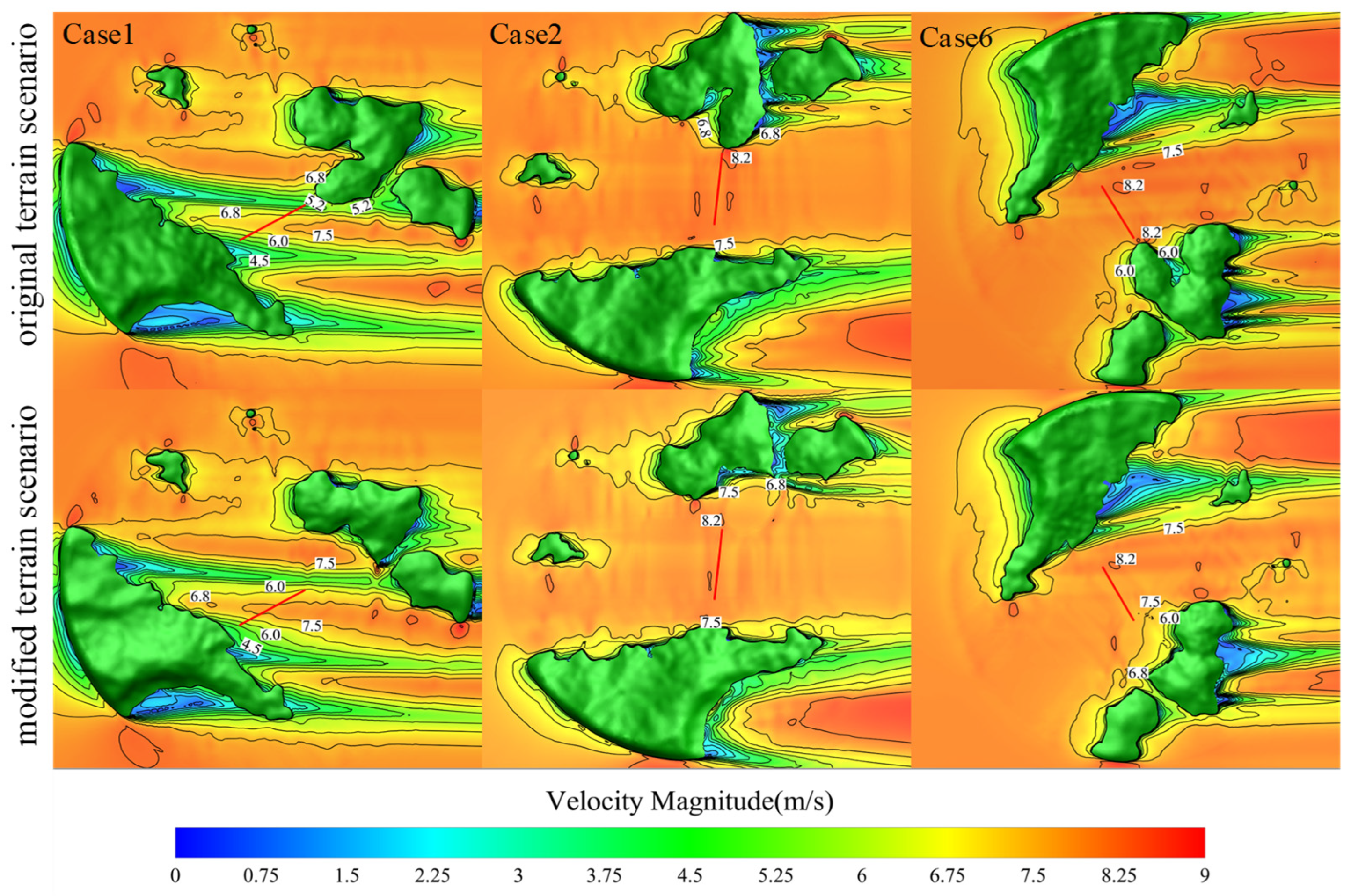
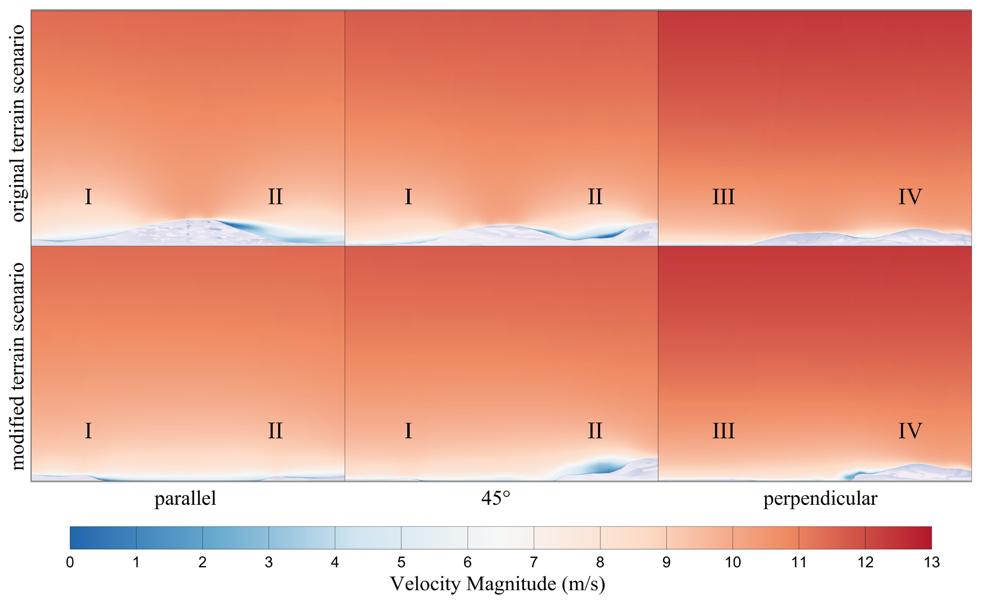
4.5. Localized Wind Effects at the Bridge Site

To further quantify the influence of local topographic variations on the wind field, this study analyzed Case 5, a scenario characterized by relatively minor discrepancies between numerical simulations and experimental measurements and a predominantly flat terrain. The maximum height of the mountain was assumed to be H (0.1 m), and six observation points were positioned around the mountain boundary along each of three orientations relative to the wind direction—specifically, “parallel”, “inclined at 45°”, and “perpendicular” (see Figure 15). The acceleration coefficient was defined as:

$$\beta ={\displaystyle \frac{V_A}{V_B}}$$

(9)

where $V_A$ and $V_B$ are the wind speeds at the same location in the modified and original terrain scenarios, respectively. By comparing $\beta$ at different heights (0.01 m, 0.1 m, and 0.2 m) and horizontal distances, we can assess how terrain changes alter local wind speeds.

Figure 16, Figure 17, Figure 18 and Figure 19 illustrate the velocity contour distributions and β value distributions under different wind directions (parallel, 45°, and perpendicular) for both the original and modified terrain conditions. The measurement points were categorized into four regions on the basis of their positions relative to the terrain: windward side (I), leeward side (II), left side (III), and right side (IV).

As shown in Figure 17, when the incoming flow was parallel to the terrain, the wind speed near the ground (0.01 m) on the windward side was approximately 20% higher in the modified terrain condition than in the original terrain condition. As the distance from the measurement point to the mountain increased to 6H, the β value gradually approached 1, indicating a significant weakening of terrain-induced disturbance effects. A similar trend was observed on the leeward side, where β decreased with increasing distance. However, at 1H, the wind speed in the modified terrain condition remained higher than that in the original condition, with an increase of up to 60% near the ground. In contrast, near 6H, the wind speed in the original terrain condition was approximately 15% higher, which is likely due to complex flows or recirculation zones. Combined with Figure 16, the windward side of the original terrain experienced localized airflow ascent and recirculation due to the mountain’s influence, resulting in reduced wind speeds near the mountain. On the leeward side, the combined effects of sheltering and vortex formation caused significant wind field disturbances, resulting in a “low near, high far” wind speed distribution pattern. Under modified terrain conditions, the wind field on the windward side became more uniform, and the flow patterns on the leeward side were simplified.

Figure 18 indicates that when the incoming flow was at a 45° angle to the terrain, the wind speed near the ground (e.g., at 1H on the windward side) in the modified terrain condition exceeded that in the original condition, suggesting a recirculation effect due to the mountain’s influence on the windward direction. At certain leeward-side measurement points, the wind speeds in the modified condition were lower than those in the original condition, particularly at low heights. However, as the observation height increased to 0.1 m and 0.2 m, the differences in β values between the two conditions diminished. Combined with the velocity contour plots, it is evident that the inclined slope of the modified terrain promotes vortex formation in the incoming flow, resulting in reduced localized wind speeds on the leeward side.

Figure 19 shows that the β values on the left side (III) were generally close to 1, indicating minimal terrain-induced disturbance and a limited influence of terrain condition changes on the wind speed. On the right side (IV), significant differences were observed near the ground, with localized high wind speed occurrences increasing under modified terrain conditions as the measurement points moved farther from the mountain boundary. Analysis of the contour plots revealed that the right side of the original terrain had a relatively gentle slope, resulting in a more uniform wind field distribution. In contrast, the modified terrain’s cut area had a steeper slope, significantly enhancing flow disturbance.

In summary, localized terrain modifications primarily affected the wind field near the ground and within a range of 1H to 3H from the mountain, with particularly complex flow patterns on the leeward side. In some instances, wind speeds in the original terrain condition exceeded those in the modified condition at specific measurement points. As the height or horizontal distance increased, the β values approached 1, indicating a marked reduction in terrain effects with increasing distance from the mountain. Therefore, in the design of nearshore long-span bridges and large-scale terrain adjustments, particular attention should be given to localized wind field variations and wind speed fluctuations within the 1H to 3H range and at low heights to avoid underestimating or overestimating the wind environment characteristics in these regions.

5. Conclusions

To investigate the influence of terrain variations near an offshore bridge site on local wind field characteristics, a study was conducted on a specific coastal bridge site. By integrating wind tunnel experiments with CFD numerical simulations, the effects of terrain variations on the wind speed, wind angle of attack, and mean wind profile at the main deck height were systematically compared under different inflow directions. Additionally, the disturbance patterns induced by local terrain-related wind effects were thoroughly examined, leading to the following key conclusions:

(1)

When the inflow direction formed a substantial angle with the mountain orientation, the mountain significantly influenced the wind field at the bridge site, producing either a pronounced shielding or acceleration effect. Under the original terrain scenario, the cross-bridge wind speed and wind angle of attack at the main girder height displayed a maximum difference of approximately 12% (increasing to as much as 25% in numerical simulations). Conversely, under the modified terrain scenario (where a portion of the mountain was removed), the wind speed distribution became more uniform, and these differences were markedly reduced. This suggests that the wind field disturbances induced by terrain variations are highly dependent on the inflow direction.

(2)

Under the original terrain scenario, the main deck angle of attack exhibited a wider fluctuation range, particularly on the side closer to the mountain, where under different wind direction conditions, both the experimental and simulation results indicated that the maximum fluctuation range was between −6° and 6°. In contrast, under the modified terrain scenario, the fluctuation range of the main deck angle of attack was significantly narrowed, suggesting that terrain variations mitigated the nonuniformity of the wind field. Under vertical inflow conditions, the influence of terrain variations on the main deck angle of attack remained relatively minor.

(3)

The impact of terrain variations on the mean wind profile was primarily concentrated in the near-ground region. At the starting point near the mountain, the wind speed under the original terrain scenario was approximately 20% lower than that under the modified terrain scenario, with simulations indicating a reduction of up to 30%. As the height increased, the wind speed disparity between the two conditions gradually diminished and ultimately converged. At locations farther from the terrain variation zone (e.g., the L/2 position), the terrain effect was significantly attenuated.

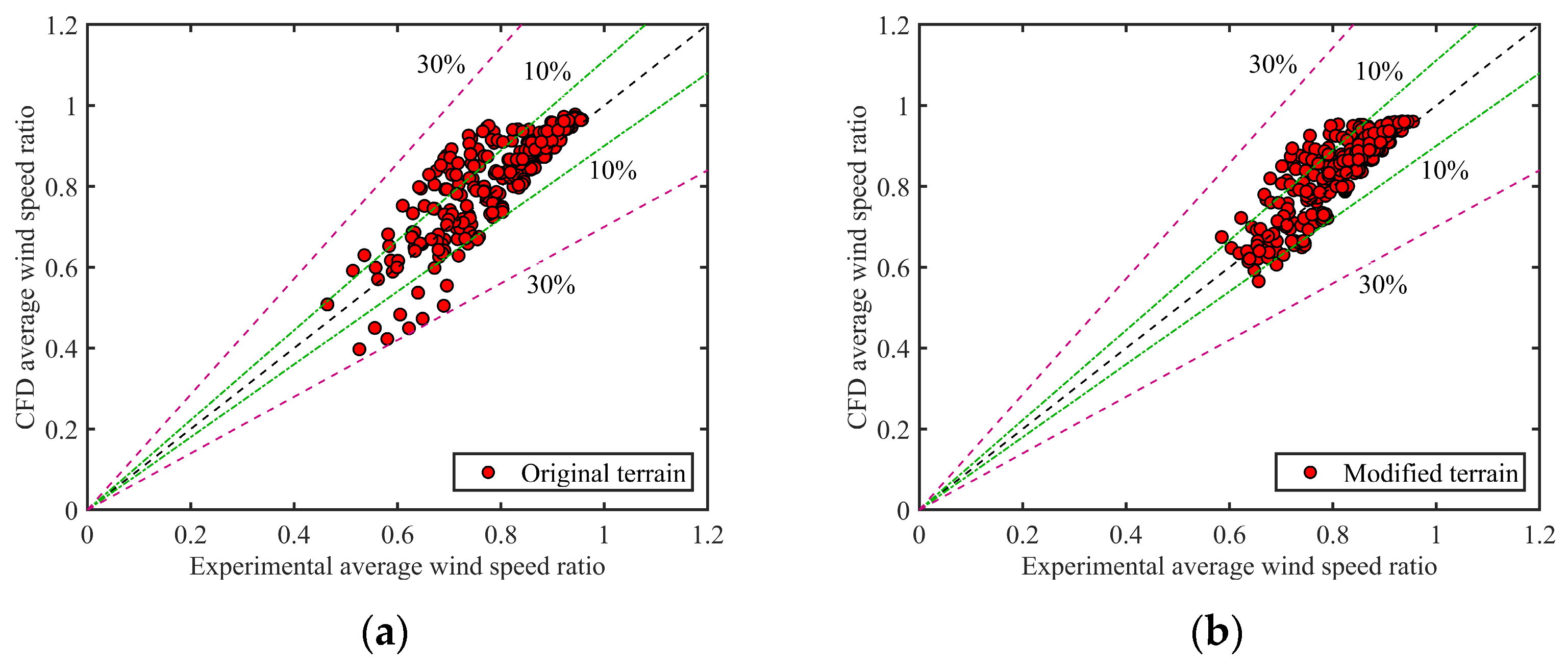
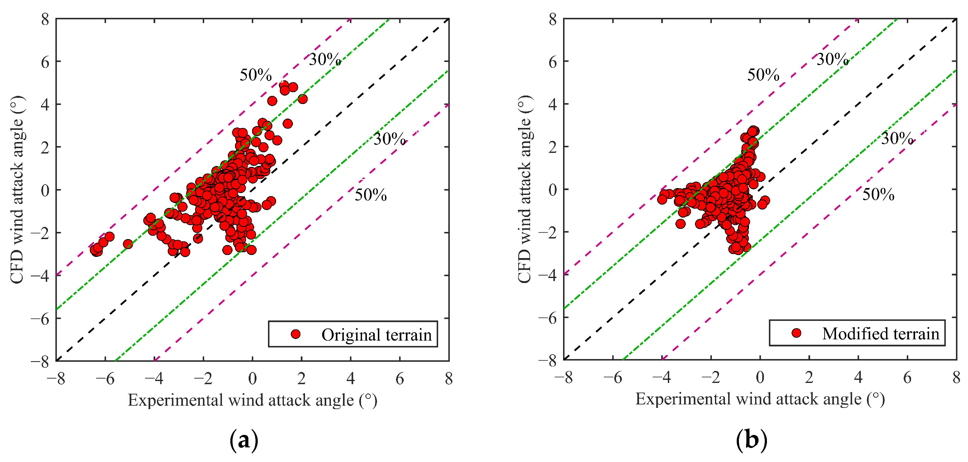
(4)

Error analysis revealed that, under the original terrain conditions, significant discrepancies existed between the numerical simulations and wind tunnel experiments for the wind speed and wind attack angle near the mountain region, with relative errors reaching 30% and 50%, respectively. In contrast, under modified terrain conditions, errors were substantially reduced, with wind speed errors controlled within ±10%, demonstrating the enhanced accuracy of numerical simulations following terrain levelling. These findings validate the reliability and engineering applicability of the SST k-ω turbulence model in simulating wind fields over complex terrain.

(5)

Numerical simulation results revealed that in the near-ground region, approximately 1H to 3H from the mountain, the local wind speed disparity between the two terrain scenarios reached as high as 60%. Notably, on the leeward side, a “reverse amplification” phenomenon emerged: at specific measurement points, the wind speed under the original terrain scenario can surpass that under the modified terrain scenario, underscoring the intricate vortex or wake effects in the leeward region.

(6)

Based on the findings of this study, future research should explore the impact of high winds (such as typhoons) on wind effects caused by terrain variations, particularly in the context of large-scale terrain modifications. For practitioners, when designing wind-resistant structures, especially bridges in coastal or mountainous areas, it is crucial to consider the impact of terrain changes on local wind conditions to ensure accurate wind load assessments and improve structural safety.

References

1. Wei, K.; Zhong, X.; Cai, H.; Li, X.; Xiao, H. Dynamic response of a sea-crossing cable-stayed suspension bridge under simultaneous wind and wave loadings induced by a landfall typhoon. Ocean. Eng. 2024, 293, 116659. [Google Scholar] [CrossRef]
2. Song, L.; Pang, J.; Jiang, C.; Huang, H.; Qin, P. Field measurement and analysis of turbulence coherence for Typhoon Nuri at Macao Friendship Bridge. Sci. China Technol. Sci. 2010, 53, 2647–2657. [Google Scholar] [CrossRef]
3. Tao, T.; Xu, Y.-L.; Huang, Z.; Zhan, S.; Wang, H. Buffeting analysis of long-span bridges under typhoon winds with time-varying spectra and coherences. J. Struct. Eng. 2020, 146, 04020255. [Google Scholar] [CrossRef]
4. Wang, H.; Li, A.; Niu, J.; Zong, Z.; Li, J. Long-term monitoring of wind characteristics at Sutong Bridge site. J. Wind Eng. Ind. Aerodyn. 2013, 115, 39–47. [Google Scholar] [CrossRef]
5. Liu, M.; Liao, H.-l.; Li, M.-s.; Ma, C.-m.; Yu, M. Long-term field measurement and analysis of the natural wind characteristics at the site of Xi-hou-men Bridge. J. Zhejiang Univ. Sci. A 2012, 13, 197–207. [Google Scholar] [CrossRef]
6. Tang, S.; Wang, K.; Yu, H.; Li, T.; Tang, J. A comparative study on wind profiles and surface aerodynamic parameters of typhoons over coastland and coastal sea. J. Geophys. Res. Atmos. 2024, 129, e2023JD040449. [Google Scholar] [CrossRef]
7. Dai, G.; Xu, Z.; Chen, Y.F.; Flay, R.G.; Rao, H. Analysis of the wind field characteristics induced by the 2019 Typhoon Bailu for the high-speed railway bridge crossing China’s southeast bay. J. Wind Eng. Ind. Aerodyn. 2021, 211, 104557. [Google Scholar] [CrossRef]
8. Zhang, J.; Zhang, M.; Li, Y.; Fang, C. Comparison of wind characteristics at different heights of deep-cut canyon based on field measurement. Adv. Struct. Eng. 2020, 23, 219–233. [Google Scholar] [CrossRef]
9. Chen, Q.; Yu, C.; Li, Y.; Zhang, X.; He, P. Directional wind characteristics analysis in the mountainous area based on field measurement. J. Wind Eng. Ind. Aerodyn. 2022, 229, 105162. [Google Scholar] [CrossRef]
10. Jing, H.; Liao, H.; Ma, C.; Tao, Q.; Jiang, J. Field measurement study of wind characteristics at different measuring positions in a mountainous valley. Exp. Therm. Fluid Sci. 2020, 112, 109991. [Google Scholar] [CrossRef]
11. Hui, M.; Larsen, A.; Xiang, H. Wind turbulence characteristics study at the Stonecutters Bridge site: Part I—Mean wind and turbulence intensities. J. Wind Eng. Ind. Aerodyn. 2009, 97, 22–36. [Google Scholar] [CrossRef]
12. Hu, P.; Li, Y.; Han, Y.; Cai, C.; Xu, G. Wind tunnel tests on the characteristics of wind fields over a simplified gorge. Adv. Struct. Eng. 2017, 20, 1599–1611. [Google Scholar] [CrossRef]
13. Kamada, Y.; Maeda, T.; Yamada, K. Wind tunnel experimental investigation of flow field around two-dimensional single hill models. Renew. Energy 2019, 136, 1107–1118. [Google Scholar] [CrossRef]
14. Meroney, R.N. Wind-tunnel simulation of the flow over hills and complex terrain. J. Wind Eng. Ind. Aerodyn. 1980, 5, 297–321. [Google Scholar] [CrossRef]
15. Jubayer, C.M.; Hangan, H. A hybrid approach for evaluating wind flow over a complex terrain. J. Wind Eng. Ind. Aerodyn. 2018, 175, 65–76. [Google Scholar] [CrossRef]
16. An, L.-S.; Alinejad, N.; Kim, S.; Jung, S. Experimental study on wind characteristics and prediction of mean wind profile over complex heterogeneous terrain. Build. Environ. 2023, 243, 110719. [Google Scholar] [CrossRef]
17. Tang, H.; Li, Y.; Shum, K.M.; Xu, X.; Tao, Q. Non-uniform wind characteristics in mountainous areas and effects on flutter performance of a long-span suspension bridge. J. Wind Eng. Ind. Aerodyn. 2020, 201, 104177. [Google Scholar] [CrossRef]
18. Zhang, M.; Zhang, J.; Li, Y.; Yu, J.; Zhang, J.; Wu, L. Wind characteristics in the high-altitude difference at bridge site by wind tunnel tests. Wind Struct. 2020, 30, 547–558. [Google Scholar]
19. Li, Y.; Hu, P.; Xu, X.; Qiu, J. Wind characteristics at bridge site in a deep-cutting gorge by wind tunnel test. J. Wind Eng. Ind. Aerodyn. 2017, 160, 30–46. [Google Scholar] [CrossRef]
20. Zou, Y.; Yue, P.; Liu, Q.; He, X.; Wang, Z. Wind field characteristics of complex terrain based on experimental and numerical investigation. Appl. Sci. 2022, 12, 5124. [Google Scholar] [CrossRef]
21. Chen, F.; Wang, W.; Gu, Z.; Zhu, Y.; Li, Y.; Shu, Z. Investigation of hilly terrain wind characteristics considering the interference effect. J. Wind Eng. Ind. Aerodyn. 2023, 241, 105543. [Google Scholar] [CrossRef]
22. Yan, L.; Guo, Z.S.; Zhu, L.D.; Flay, R.G. Wind tunnel study of wind structure at a mountainous bridge location. Wind Struct. 2016, 23, 191–209. [Google Scholar] [CrossRef]
23. Li, Y.; Xu, X.; Zhang, M.; Xu, Y. Wind tunnel test and numerical simulation of wind characteristics at a bridge site in mountainous terrain. Adv. Struct. Eng. 2017, 20, 1223–1231. [Google Scholar] [CrossRef]
24. Zhang, M.; Yu, J.; Zhang, J.; Wu, L.; Li, Y. Study on the wind-field characteristics over a bridge site due to the shielding effects of mountains in a deep gorge via numerical simulation. Adv. Struct. Eng. 2019, 22, 3055–3065. [Google Scholar]
25. Song, J.-L.; Li, J.-W.; Flay, R.G.; Pirooz, A.A.S.; Fu, J.-Y. Validation and application of pressure-driven RANS approach for wind parameter predictions in mountainous terrain. J. Wind Eng. Ind. Aerodyn. 2023, 240, 105483. [Google Scholar] [CrossRef]
26. Zhu, X.-q.; Weng, J.-t.; Wu, Y.-q.; Gao, W.-j.; Wang, Z. Wind suitability in site analysis of coastal concave terrains using computational fluid dynamics simulation: A case study in East Asia. J. Zhejiang Univ. -Sci. A 2017, 18, 741–756. [Google Scholar] [CrossRef]
27. Abdi, D.S.; Bitsuamlak, G.T. Wind flow simulations on idealized and real complex terrain using various turbulence models. Adv. Eng. Softw. 2014, 75, 30–41. [Google Scholar] [CrossRef]
28. Chen, X.; Liu, Z.; Wang, X.; Chen, Z.; Xiao, H.; Zhou, J. Experimental and numerical investigation of wind characteristics over mountainous valley bridge site considering improved boundary transition sections. Appl. Sci. 2020, 10, 751. [Google Scholar] [CrossRef]
29. Nabil, M.; Guo, F.; Jiang, L.; Yu, Z.; Long, Q. Numerical Investigation of Wind Flow and Speedup Effect at a Towering Peak Extending out of a Steep Mountainside: Implications for Landscape Platforms. Mathematics 2024, 12, 467. [Google Scholar] [CrossRef]
30. Song, J.-L.; Li, J.-W.; Xu, R.-Z.; Flay, R.G. Field measurements and CFD simulations of wind characteristics at the Yellow River bridge site in a converging-channel terrain. Eng. Appl. Comput. Fluid Mech. 2022, 16, 58–72. [Google Scholar] [CrossRef]
31. Hu, P.; Li, Y.; Han, Y.; Cai, S.C.; Xu, X. Numerical simulations of the mean wind speeds and turbulence intensities over simplified gorges using the SST k-ω turbulence model. Eng. Appl. Comput. Fluid Mech. 2016, 10, 359–372. [Google Scholar] [CrossRef]
32. Yang, W.; Quan, Y.; Jin, X.; Tamura, Y.; Gu, M. Influences of equilibrium atmosphere boundary layer and turbulence parameter on wind loads of low-rise buildings. J. Wind Eng. Ind. Aerodyn. 2008, 96, 2080–2092. [Google Scholar] [CrossRef]
33. Yang, Y.; Xie, Z.; Gu, M. Consistent inflow boundary conditions for modelling the neutral equilibrium atmospheric boundary layer for the SST k-ω model. Wind Struct. 2017, 24, 465–480. [Google Scholar] [CrossRef]
34. JTG/T 3360-01—2018; Wind-Resistant Design Specification for Highway Bridges. Tongji University: Shanghai, China, 2019.
Figure 1. Comparison of the terrain models under two scenarios: (a) original terrain scenario; (b) modified terrain scenario.
Jmse 13 01223 g001
Figure 2. Bridge layout, terrain information, and incoming wind directions: (a) bridge layout; (b) topographic elevation; (c) schematic of incoming wind conditions.
Jmse 13 01223 g002
Figure 3. Terrain models for the two scenarios in the wind tunnel: (a) original terrain scenario; (b) modified terrain scenario.
Jmse 13 01223 g003
Figure 4. Vertical distributions of the wind speed and turbulence intensity: (a) wind speed profile; (b) turbulence intensity.
Jmse 13 01223 g004
Figure 5. Computational domain, boundary conditions, and grid for the comparative terrain scenario.
Jmse 13 01223 g005
Figure 6. Comparison of the mean wind characteristics under different mesh conditions: (a) transverse wind velocity at the main deck; (b) angle of attack at the main deck; (c) longitudinal wind velocity profiles.
Jmse 13 01223 g006
Figure 7. Velocity and turbulent kinetic energy fitting curves: (a) velocity fitting curve; (b) turbulent kinetic energy fitting curve.
Jmse 13 01223 g007
Figure 8. Equilibrium atmospheric boundary layer (ABL) validation results: (a) computational domain grid; (b) comparison of inlet and outlet wind profiles; (c) velocity contour map.
Jmse 13 01223 g008
Figure 9. Transverse wind velocity at the main deck height under different wind directions: (a) Case 1; (b) Case 2; (c) Case 3; (d) Case 4; (e) Case 5; (f) Case 6.
Jmse 13 01223 g009
Figure 10. Velocity cloud maps at the main deck height under typical scenarios.
Jmse 13 01223 g010
Figure 11. Angle of attack at the main deck height under different wind directions: (a) Case 1; (b) Case 2; (c) Case 3; (d) Case 4; (e) Case 5; (f) Case 6.
Jmse 13 01223 g011
Figure 12. Numerical and experimental results of average wind velocity ratio profiles under typical wind conditions: (a) starting point; (b) L/4; (c) L/2.
Jmse 13 01223 g012
Figure 13. Numerical and experimental results of the transverse wind velocity at the main deck height under different wind directions: (a) original terrain; (b) modified terrain.
Jmse 13 01223 g013
Figure 14. Numerical and experimental results of the angle of attack at the main deck height under different wind directions: (a) original terrain; (b) modified terrain.
Jmse 13 01223 g014
Figure 15. Layout of measurement points for localized wind effect analysis.
Jmse 13 01223 g015
Figure 16. Comparison of localized velocity cloud maps of mountains in the modified/original terrain.
Jmse 13 01223 g016
Figure 17. Acceleration factors for measurement points along the horizontal (parallel) direction.
Jmse 13 01223 g017
Figure 18. Acceleration factors for measurement points 45° to the inflow.
Jmse 13 01223 g018
Figure 19. Acceleration factors for measurement points in the perpendicular direction.
Jmse 13 01223 g019